Article

Multi-Size Proppant Pumping Schedule of Hydraulic Fracturing: Application to a MP-PIC Model of Unconventional Reservoir for Enhanced Gas Production

1
Artie McFerrin Department of Chemical Engineering, Texas A&M University, College Station, TX 77845, USA
2
Texas A&M Energy Institute, Texas A&M University, College Station, TX 77845, USA
3
Department of Petroleum Engineering, Texas A&M University, College Station, TX 77845, USA
*
Author to whom correspondence should be addressed.
Submission received: 17 March 2020 / Revised: 30 April 2020 / Accepted: 2 May 2020 / Published: 12 May 2020
(This article belongs to the Special Issue Modeling, Control, and Optimization of Batch and Batch-Like Processes)

Abstract

:
Slickwater hydraulic fracturing is becoming a prevalent approach to economically recovering shale hydrocarbon. It is very important to understand the proppant’s transport behavior during slickwater hydraulic fracturing treatment for effective creation of a desired propped fracture geometry. The currently available models are either oversimplified or have been performed at limited length scales to avoid high computational requirements. Another limitation is that the currently available hydraulic fracturing simulators are developed using only single-sized proppant particles. Motivated by this, in this work, a computationally efficient, three-dimensional, multiphase particle-in-cell (MP-PIC) model was employed to simulate the multi-size proppant transport in a field-scale geometry using the Eulerian–Lagrangian framework. Instead of tracking each particle, groups of particles (called parcels) are tracked, which allows one to simulate the proppant transport in field-scale geometries at an affordable computational cost. Then, we found from our sensitivity study that pumping schedules significantly affect propped fracture surface area and average fracture conductivity, thereby influencing shale gas production. Motivated by these results, we propose an optimization framework using the MP-PIC model to design the multi-size proppant pumping schedule that maximizes shale gas production from unconventional reservoirs for given fracturing resources.

1. Introduction

Hydraulic fracturing is a well stimulation technique to enhance shale gas production from unconventional reservoirs in the petroleum industry [1,2,3]. During hydraulic fracturing, highly pressurized fracturing fluids are pumped to create fractures which provide highly conductive paths for shale gas to flow from reservoirs to the wellbores. Proppant (e.g., sand, alumina, or zirconia) carried by the injected fracturing fluid will prevent the fracture from closing and maintain the high conductivity of propped fracture during shale gas production [4]. Because of extensive use of hydraulic fracturing over the last decade in the United States, production of shale gas from unconventional reservoirs has increased from 5.7 trillion cubic feet in 2000 to over 26 trillion cubic feet in 2019.
In hydraulic fracturing, proppant transport takes place along the horizontal direction by the fracturing fluid, and along the vertical direction by the gravitational settling. In unconventional reservoirs, slickwater is widely used as the fracturing fluid due to its advantages such as low cost and reduced gel damage [5]. However, due to the low-viscosity of slickwater, the proppant settles quickly and forms a proppant bank, which results in a short propped fracture length. Therefore, it is very important to understand the proppant transport behavior during slickwater hydraulic fracturing treatment to effectively create a desired propped fracture geometry.
Many experimental studies have been conducted to understand the proppant transport process with the aim of achieving improved fracture conductivity. Specifically, slots have been used to investigate the effects of fracturing fluid and fracture geometry on the proppant distribution in a single fracture [6,7,8]. Wang et al. (2003) [9] conducted slot experiments to derive bi-power law correlations for bed load proppant transport during hydraulic fracturing using slickwater. In some of the unconventional reservoirs, naturally present fractures will interact with hydraulic fractures and result in complex fracture geometries. In order to understand the proppant transport in a complex fracture network, many experimental studies have been conducted recently using complex slot configurations [10,11,12]. However, all these experimental studies are performed at lab-scales, and thus, these results cannot be directly applied to field-scale hydraulic fracturing.
In order to simulate field-scale proppant transport, the Eulerian–Lagrangian method and Eulerian–Eulerian method have been widely considered. In the Eulerian–Eulerian method, both the fracturing fluid and proppant are solved in Eulerian grids using continuum governing equations [13,14,15]. These continuum models are developed to quickly solve proppant transport, but they cannot capture the discrete characteristics of proppants. In addition, for multi-size proppant pumping schedules, one has to treat particles with different sizes or materials as separate phases, which may require solving additional continuity and momentum equations [16].
In the Eulerian–Lagrangian method, the Lagrangian method is used to solve proppant transport, and Eulerian grids are used to solve the fracturing fluid flow [17,18,19,20]. Compared to the Eulerian–Eulerian framework, the Eulerian–Lagrangian framework can consider multi-size proppant pumping schedules; the latter is computationally more demanding than the former. Within the Eulerian–Lagrangian framework, two models are widely used for proppant transport simulation: the computational fluid dynamics-discrete element method (CFD-DEM) and the multiphase particle-in-cell (MP-PIC) method. The main difference between these two methods is how to deal with the dispersed phase (i.e., proppant particles). In CFD-DEM models, each individual particle is treated separately, and the velocity and position of every particle are calculated by integrating the forces acting on them over time. While this approach is effective in capturing proppant transport at relatively small scales, it is difficult to apply this method to field-scale simulations because of its extremely high requirement of computation power. In MP-PIC models, the dispersed phase is approximated by many parcels; each parcel contains a group of proppant particles. Because of these characteristics, MP-PIC models are able to capture the important features of proppant transport in field-scale geometries at a greatly reduced computational cost.
While the MP-PIC approach has been widely adopted in other particulate systems [16,21,22,23,24,25], its application to multiphase oil/gas systems has not received much attention. Motivated by recent developments [26,27,28], a three-dimensional MP-PIC model has been employed to simulate the proppant transport behavior in a field-scale geometry. In hydraulic fracturing, it is very important to achieve the required fracture geometry, as it will maximize shale gas production rate from unconventional reservoirs [29]. Recently, several studies have been conducted to compute pumping schedules to achieve an optimal fracture geometry [14,29,30,31,32,33,34,35,36,37,38]. However, these pumping schedules are developed using single-sized proppant particles, and the effect of multi-size proppant pumping schedules on the performance of hydraulic fracturing still remains unclear. In the case of unconventional reservoirs, shale gas production depends on propped fracture surface area (PFSA) and average fracture conductivity (AFC). Therefore, it is very important to achieve desired PFSA and AFC values by manipulating the pumping schedule (i.e., fracturing fluid flow rate, proppant concentration, and proppant size injected at the wellbore). In this regard, we use a MP-PIC model within an optimization framework to compute the optimal multi-size proppant pumping schedule that maximizes shale gas production from unconventional reservoirs for given fracturing resources (i.e., proppant amount, etc.).
This paper is organized as follows: In Section 2, we describe a MP-PIC model. In Section 3, we apply the MP-PIC model to a field-scale fracture geometry and demonstrate the importance of considering multi-size proppant pumping schedules. In Section 4, we apply the MP-PIC model within an optimization framework to determine the multi-size proppant pumping schedule that maximizes shale gas production from unconventional reservoirs for given fracturing resources. In Section 5, we present several simulation results to show increased productivity obtained by the computed pumping schedule.

2. High-Fidelity Model Formulation Using the MP-PIC Model

If the MP-PIC method is applied to hydraulic fracturing, mass and momentum equations are solved to describe the fracturing fluid behavior, treating it as a continuous phase, and the Lagrangian description is used to solve Liouville equation to describe the proppant transport behavior. Further, instead of tracking each particle like in CFD-DEM, a group of particles (called a parcel) is tracked, and the particles within each parcel are presumed to have an identical density, volume, velocity, and position (Figure 1). The governing equations for the fluid and particle phases are described below.

2.1. Fluid Phase

The following mass and momentum equations are used to describe the fluid phase.
α f ρ f t + · α f ρ f u f = 0
α f ρ f u f t + · α f ρ f u f u f = p F f p + α f ρ f g + · α f τ f
where
S i j = 1 2 u i x j + u j x i
ϕ ( x , u p , ρ p , V p , t )
α p = ϕ V p d V p d ρ p d u p
α f = 1 ϕ V p d V p d ρ p d u p
τ i j = 2 μ f S i j 2 3 μ f δ i j u i x j
where subscripts f and p are used to denote the fluid and particle phases, respectively; u f is the fluid velocity; ∇ is the vector differential operator; ρ f is the fluid density; F f p is the rate of momentum exchange between the fluid phase and particle phase; p is the fluid pressure; g is the gravitational acceleration constant; α p and α f are the proppant particle and fluid volume fractions, respectively; τ i j is the fluid phase stress tensor; and μ f is the fluid viscosity [26,27].

2.2. Particle Phase

Particle distribution function, ϕ ( x , u p , ρ p , V p , t ) , is used to describe the dynamics of the particle phase, where x is the particle position, u p is the particle velocity, ρ p is the particle density, V p is the particle volume, and t is the current time. The time evolution of ϕ is obtained by solving the Liouville equation while simultaneously considering drag force, pressure gradient, gravity, and inter-particle stress, which is given by [21]:
ϕ t + · ϕ u p + u p · ϕ A = 0
where
A = d u p d t = D p ( u f u p ) 1 ρ p p + g 1 α p ρ p τ p
where A is the proppant parcel acceleration, D p is the drag coefficient, and τ p is the inter-particle stress. On the right hand side in Equation (5), the first term is the interface drag force, the second term is the dynamic pressure gradient, the third term is the acceleration due to gravity, and the fourth term is the acceleration due to inter-particle stress. D p is determined by using the drag force model developed by [39], which is given below:
D p = C d 3 8 ρ f ρ p u f u p R p
where
C d = 24 R e α f 2.65 + R e 2 / 3 6 α f 1.78 R e < 1000 0.44 α f 2.65 R e > 1000
R e = 2 ρ f u f u p r p μ f
r p = 3 V p 4 π 1 / 3
where C d is the dimensionless drag force coefficient, R e is the Reynolds number, and r p is the proppant particle radius. The inter-particle stress for particle-particle collision is calculated using the following equation [40]:
τ p = P s α p β α c p α p
where β is a constant between 2 and 5, P s is another constant, and α c p is the proppant parcel volume fraction at closed packing. Mao et al. (2020) [27] conducted slot experiments to validate the MP-PIC model. The values of β and P s were chosen as 2 and 4 Pa, respectively, to achieve a good fit between the experimental data and MP-PIC model. More details regarding the MP-PIC model validation can be found in Mao et al. (2020) [27].

2.3. Propped Fracture Conductivity

We can obtain the spatio-temporal profile of proppant concentration, c ( x , y , t ) = α p ( x , y , t ) , by solving Equations (1)–(8). However, in order to measure the permeability of a fracture, we need to determine the fracture conductivity, which is defined as the product of proppant bank permeability and fracture width. Fracture permeability, k, is determined by the Kozeny–Carman relation [41], which is given below:
k = α f 3 C S 2 ( 1 α f ) 2
where C is the Kozeny–Carman constant which is taken as 5 for unconsolidated sand pack, and S is the proppant particle surface per unit volume of proppant bank. Fracture conductivity, C f d , is determined for a given fracture width W f and S, using the following equation:
C f d = 1.1 × 10 10 W f S 2 α f 3 ( 1 α f ) 2
The coefficient in Equation (10) is the unit conversion factor between the fracture conductivity, C f d , which is in md·ft; and fracture width ( W f ) and the proppant particle surface per unit volume of proppant bank, S, both of which are in inches.

2.4. Reservoir Simulator

The reservoir simulation software from Computer Modeling Group Ltd. (CMG, Calgary, AB, Canada) is used to simulate shale gas production from an unconventional reservoir. The spatial profiles of fracture conductivity and the propped fracture geometry (i.e., the propped average fracture width, propped fracture length, and propped fracture height) obtained from the MP-PIC model at the end of hydraulic fracturing are fed as inputs to CMG software to simulate shale gas production from a well in a unconventional reservoir using a single fracture. A flowchart describing the computational procedures between the MP-PIC model and CMG is given in Figure 2.
Remark 1.
Zeng et al. (2019) [28] developed a model by coupling a two-dimensional MP-PIC method with the Perkins–Kern–Nordgren (PKN) fracture propagation model to study the proppant transport process. In our work, a three-dimensional MP-PIC model developed by Mao et al. (2019) [26] was employed to simulate the proppant transport behavior in a field-scale geometry. More details regarding the implementation of the MP-PIC model can be found in Mao et al. (2019) [26]. We use the MP-PIC model as a virtual experiment to generate data and use the data to develop a mathematical formulation to find the pumping schedule that maximizes the shale gas production from a shale gas well. The major contribution of this work is not developing the MP-PIC model but using the model to develop a multi-size proppant pumping schedule technique for optimal operation of a shale gas well.
Remark 2.
In the MP-PIC model, we considered several particles of identical density, volume, velocity, and specific position as a computational parcel. The particle motion is governed by Newton’s second law. The forces affecting the particles’ motion are fluid-particle drag, gravity, dynamic pressure gradient, and particle stress. When calculating these terms, we consider the velocity and acceleration of the particulate phase. The particle size will play an important role when we calculate the fluid particle drag because the drag coefficient is related to the particle size. Additionally, when we calculate the particle volume fraction, we need to sum up all the physical particle volumes within the Eulerian cell.
Remark 3.
Mao et al. (2020) [27] conducted slot experiments to validate the MP-PIC model. The predicted proppant concentration and proppant bank height profiles were very close to experimental data, which verified that the theory was implemented correctly. More details regarding the MP-PIC model validation can be found in Mao et al. (2020) [27].

3. Field-Scale Simulation Results Using the MP-PIC Model

In this section, by varying the proppant pumping schedule, we study its effect on the proppant transport behavior in a field-scale fracture geometry using the MP-PIC model. The fluid flow and proppant transport were fully coupled, and we used the open source computational fluid dynamics software, OpenFOAM, to simulate fluid flow and proppant transport. The parameters used in the MP-PIC model are given in Table 1. Since the fracture is symmetrical, we only modeled a half-fracture using the computation cell configuration shown in Figure 3. The considered fracture geometry is comparable to a field-scale; in particular, a fracture of 180 m in half-length, 30 m in height, and 0.00762 m in width is considered. In the fracture width direction, we considered only one cell because of the high aspect ratio (length over width) of the fracture. The fracturing fluid is injected at the beginning of the half fracture (x = 0) and through the center along the vertical direction (y = 13.5 m to 16.5 m).
The MP-PIC model was simulated using the Ada and Terra clusters provided by Texas A&M high performance research computing facility. The MP-PIC method required around 96 h of calculation via 28 CPUs to simulate proppant transport in the described field-scale fracture geometry. In the literature, available CFD-DEM simulations only considered the fracture length to be up to 10 m, which is much smaller than field-scale fracture geometries; and fracturing fluid injection time to be up to 200 s, which is also not a field-scale injection time [19]. Because of the gain in computational efficiency by the use of the MP-PIC method, we were able to simulate proppant transport in the field-scale fracture geometry.
Then, we studied the effect of proppant size on proppant transport using the fracture configuration shown in Figure 3. For this analysis, we used two different proppant sizes: 100 mesh (150 μm) and 40 / 70 mesh (320 μm). This study was performed through three field-scale case studies (denoted as A, B, and C) using three different pumping schedules with a fixed fracturing fluid flow rate of 10 bbl/min and total proppant amount of M p r o p = 31,500 lb, which are presented in Figure 4. In Case A, we considered the pumping schedule in which the mass percentage of 150 μm proppant is 30%. In Case B and Case C, we varied the mass percentage of 150 μm proppant to 50% and 70%, respectively, by adjusting the injection time of each pumping stage. The overall operation of hydraulic fracturing is for 1 h, and the proppant density is 2650 kg/m 3 .
These three pumping schedules were applied to the MP-PIC model. The final proppant concentration distributions are presented in Mao et al. (2020) [27], and it is clear that the proppant transport behavior is highly sensitive to the fracturing fluid flow rate, proppant concentration, and proppant size used during injection. More specifically, it was observed that in Case C, the proppant particles travel farther than the other two cases, wherein the mass percentages of smaller size proppant particles are higher. This is because the gravitational settling of smaller proppant particles is less substantial and can be easily carried deeper into the fracture by the fracturing fluid. In Case A, the proppant particles do not travel much due to their large size, which results in significant gravitational settling, and thereby a short proppant bank.
After obtaining the final proppant concentration distribution, we then calculated the fracture conductivity profile across the fracture for these cases using Equations (9) and (10), as shown in Mao et al. (2020) [27]. It was observed that in Case A, the high fracture conductivity region was mainly due to the high mass percentage of large proppant particles (i.e., high-permeability proppant). On the other hand, in Case C, the fracture conductivity was relatively low due to the presence of small proppant particles (i.e., low-permeability proppant).
After obtaining the fracture conductivity profile and the propped fracture geometry, we then simulated shale gas production using the CMG reservoir simulator for these three cases. Table 2 summarizes the AFC, PFSA, and the cumulative shale gas production volume obtained using these pumping schedules. Our results indicated that pumping schedules significantly affect PFSA and AFC, and thereby the cumulative shale gas production volume from unconventional reservoirs. It is observed that using a pumping schedule with a high mass percentage of small size proppant particles (Case C) results in a large PFSA because proppants can penetrate deep inside the fracture due to insignificant gravitational settling. On the other hand, using a pumping schedule with a high mass percentage of large size proppant particles (Case A) results in a high AFC due to the high permeability of large proppant particles. The cumulative shale gas production volume at the end of 10 years is the greatest in Case B, wherein equal mass percentages of small and large proppant particles are used.
The above results show that it is very important to achieve desired PFSA and AFC values to maximize the cumulative shale gas extraction volume from unconventional reservoirs through the manipulation of the pumping schedule (i.e., fracturing fluid flow rate, proppant concentration, and proppant size injected at the wellbore). Motivated by this, we propose an optimization framework in the following section to obtain the pumping schedule that maximizes the cumulative shale gas production volume from unconventional reservoirs by achieving desired PFSA and AFC values for given fracturing resources (i.e., proppant amount, etc.).

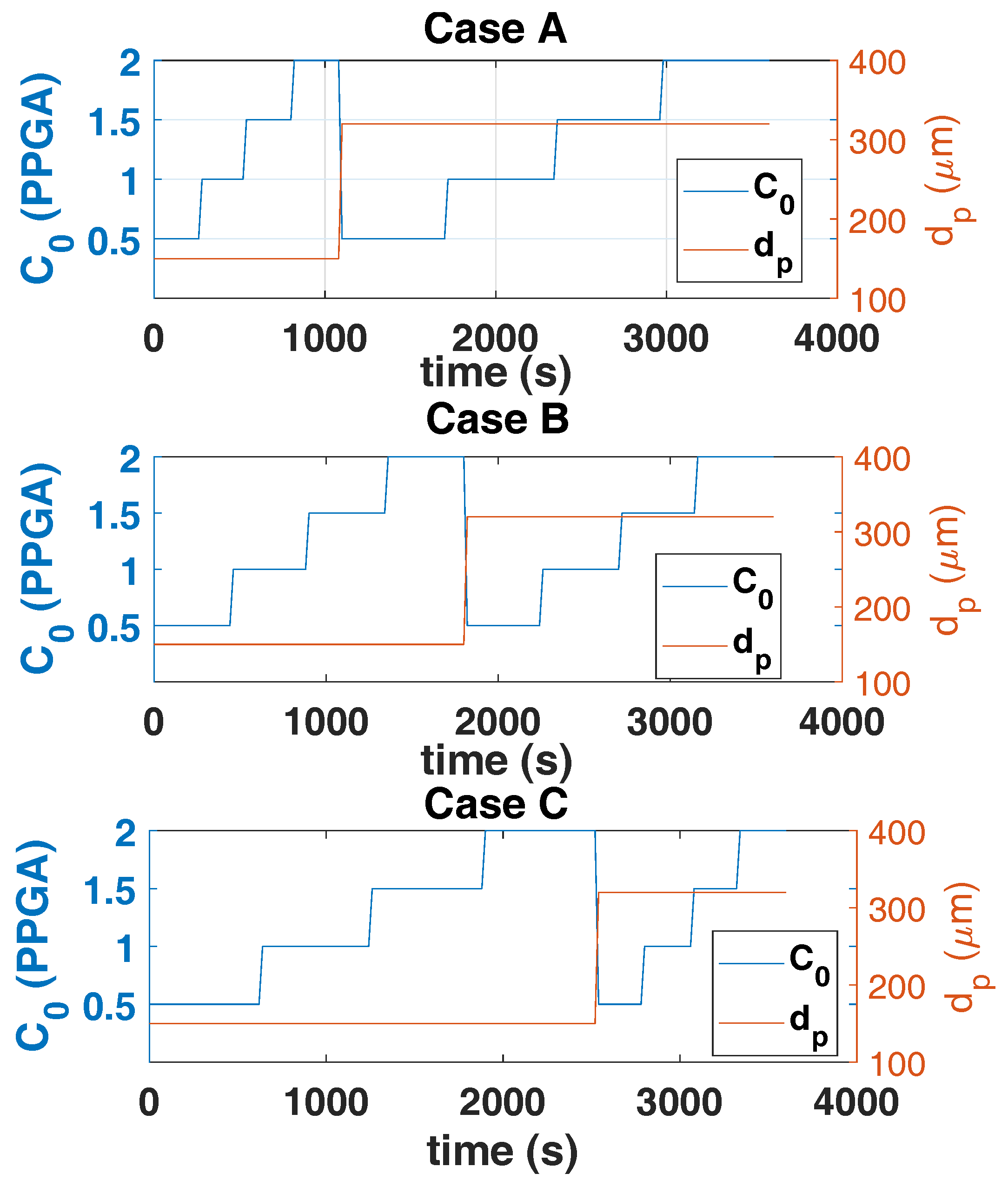
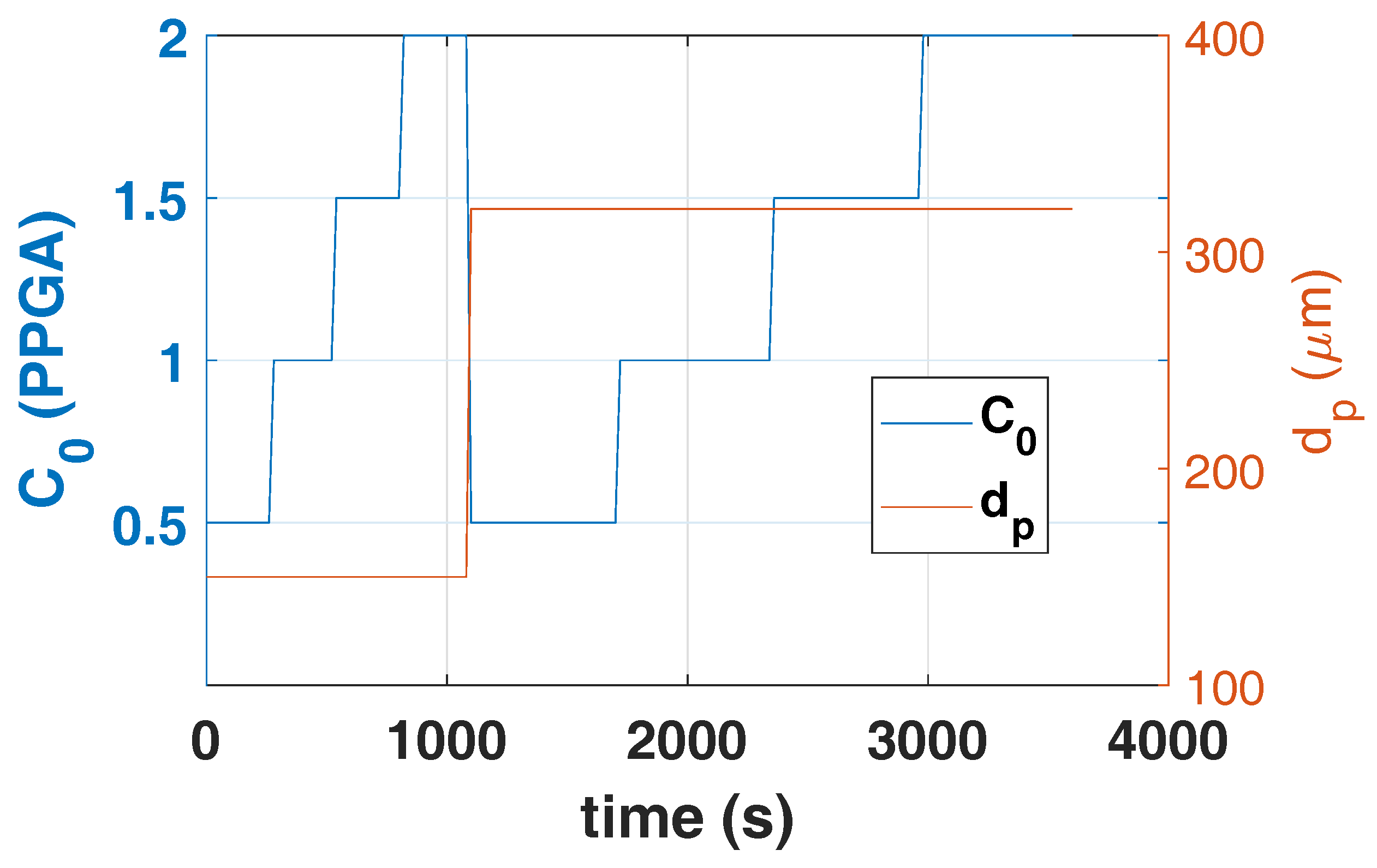
4. Optimal Operation of Hydraulic Fracturing Using the MP-PIC Model

Before we compute an optimal multi-size proppant pumping schedule using the MP-PIC model, we present the currently available pumping schedule design techniques and their drawbacks.

4.1. Background on Existing Pumping Schedules

A power-law type pumping schedule for proppant concentration with a fixed fracturing fluid flow rate was proposed by Nolte (1986) [42], which is one of the most commonly used techniques in the oil and gas industry. However, Nolte’s pumping schedule has some limitations: (1) it does not consider all the phenomena that happen during hydraulic fracturing, particularly proppant settling due to gravity; (2) it only considers single fracture propagation; (3) the form of pumping schedule is predefined and applied in an open-loop manner to create a single hydraulic fracture, which may result in early termination of hydraulic fracturing when there is a plant-model mismatch.
To deal with the limitations of Nolte’s pumping schedule, Gu and Desroches (2003) [43] developed a pumping schedule design technique using a hydraulic fracturing simulator. Specifically, an iterative method is used to solve an inverse problem to achieve a desired fracture length and distribution of proppant by manipulating the proppant concentration in pumping schedules. Dontsov and Peirce (2014) [44] developed another pumping schedule design technique to improve Nolte’s pumping schedule; however, they neglected the relationship between proppant concentration and fracture propagation. Recently, Siddhamshetty et al. (2019) [37] developed a new model-based control system to compute a fracturing fluid pumping schedule by mitigating the stress-shadow effects in simultaneously-growing fractures to achieve a desired fracture geometry. Siddhamshetty et al. (2020) [45] further extended their previous work to maximize the total fracture surface area in naturally fractured unconventional reservoirs. However, all of these pumping schedules are developed using single-sized proppant particles, and the effect of multi-size proppant pumping schedules on the performance of hydraulic fracturing was not investigated. In summary, while it is very important to achieve desired PFSA and AFC values to maximize shale gas extraction from unconventional reservoirs, as shown in Section 3, they were not considered in these pumping schedule design techniques.
To address this limitation, we have formulated an optimization problem in the following subsection. The MP-PIC method presented in Section 2 requires running 28 CPUs for 96 h to simulate proppant transport in a field-scale fracture geometry. Because of the large computational requirement, although it is much more affordable than other CFD-DEM models, it cannot be directly used in this optimization problem for the computation of an optimal multi-size proppant pumping schedule. After hydraulic fracturing, we used CMG reservoir simulator to predict shale gas production at the end of 10 years, which again requires huge computational resources. Therefore, it is necessary to develop computationally efficient models to approximate the MP-PIC model and CMG reservoir simulator, which is presented in the following subsection.

4.2. Handling the Computational Requirement of the MP-PIC Model

In this subsection, we developed two computationally efficient models which will be used in the optimization framework to reduce the computational requirements of the MP-PIC model and CMG simulator (Figure 5). The first model is a multi-variable output error state-space (MOESP)-based reduced-order model (ROM) that describes the relationships between the manipulated input variables (i.e., proppant concentration, and proppant size injected at the wellbore) and the output variables (i.e., PFSA and AFC) of the MP-PIC model. In the following subsections, we first describe how this ROM is developed by utilizing data generated from the MP-PIC model.

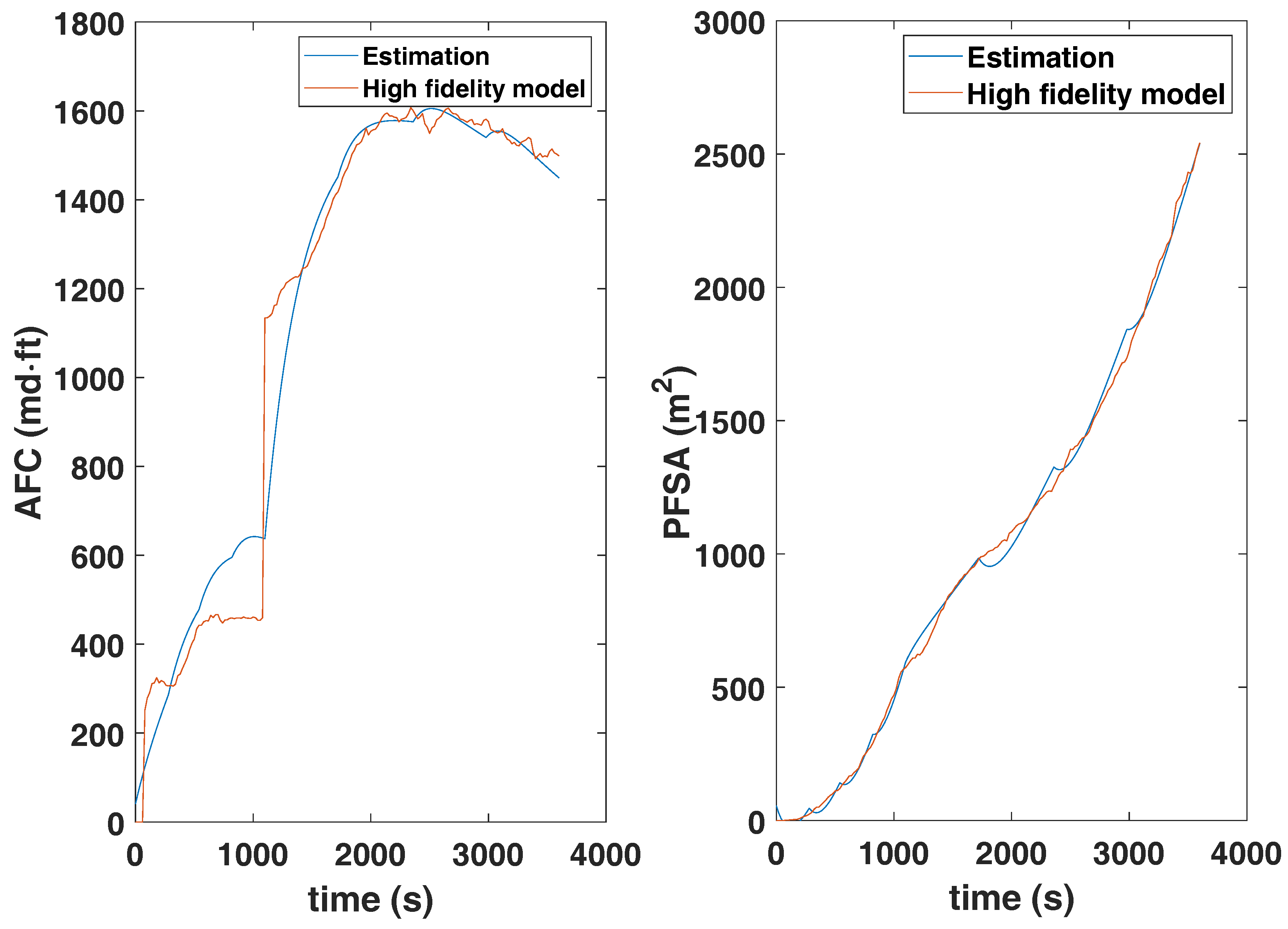
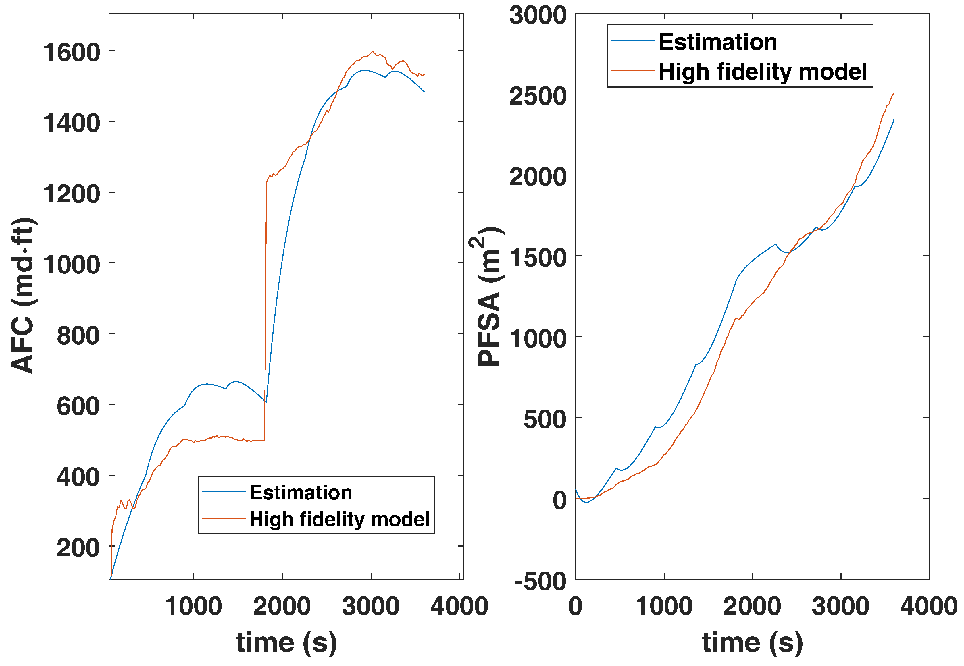
4.2.1. ROM to Simulate the Hydraulic Fracturing Process

In this subsection, we develop a ROM using MOESP algorithm to describe the proppant transport phenomena during hydraulic fracturing, which is given below:
x ( t k + 1 ) = A x ( t k ) + B u ( t k )
y ( t k ) = C x ( t k )
where u ( t k ) = [ C x 0 ( t k ) , d p ( t k ) ] T are the input variables, where C x 0 ( t k ) and d p ( t k ) are the proppant concentration and proppant size injected at the wellbore, respectively; y ( t k ) = [ P F S A ( t k ) , A F C ( t k ) ] are the output variables; and x ( t k ) are the ROM states. We have used the data generated from the MP-PIC model to determine the model parameters A, B, and C, and the initial state estimate, x ( 0 ) .
We carried out open-loop simulations by applying a training input (Figure 6) to the MP-PIC model. Utilizing these simulation data, we obtained an ROM, which is a 3rd-order, linear, time-invariant, state-space model. The training input is chosen by considering the minimum and maximum allowable fracturing proppant concentration and proppant size. We have used two different proppant sizes, 100 mesh (150 μm) and 40/70 mesh (320 μm), and considered a non-decreasing trend with respect to the injected proppant concentration, as shown in Figure 6. We observed in Figure 7 that PFSA and AFC obtained from the ROM are close to the values obtained from the MP-PIC model.
We then validated the ROM by using different pumping schedules (Figure 8). The performance of the ROM for the validation pumping schedules is shown in Figure 9, where it is observable that PFSA and AFC obtained from the ROM are close to the true values from the MP-PIC model.

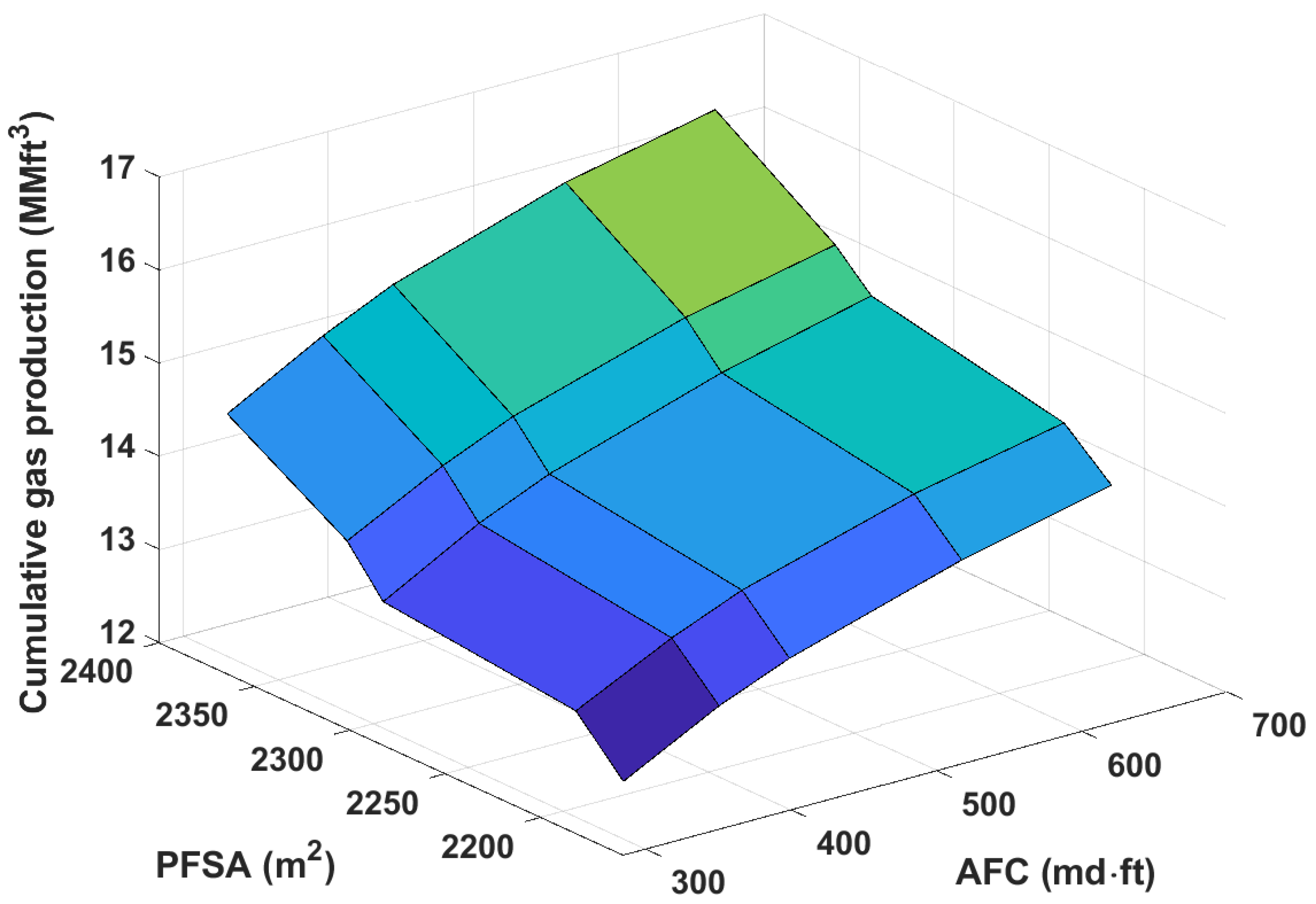
4.2.2. Map to Correlate the Fracture Properties to the Cumulative Gas Production Volume

In this work, we have used CMG reservoir simulator to compute cumulative shale gas production volumes using final fracture properties and geometry at the end of hydraulic fracturing process. Specifically, we have used a package called GEM available in CMG simulator to model shale gas production by providing the component properties and the rock-fluid properties of a shale reservoir. The inputs to CMG-GEM are AFC and PFSA. We used a variety of AFC and PFSA values as inputs to CMG-GEM to generate the corresponding shale gas production profiles. Using the input (PFSA and AFC) and output (cumulative shale production at the end of 10 years) data, we developed a map (Figure 10) where the x-axis is AFC, y-axis is PFSA, and z-axis is the cumulative shale gas production volume at the end of 10 years. There is a general trend that shale gas production increases with PFSA and AFC.

4.3. Optimization Framework to Maximize Cumulative Shale Gas Production Volume from Unconventional Reservoirs

In this subsection, we propose an optimization framework to compute the optimal multi-size proppant pumping schedule that maximizes the cumulative shale gas production volume from unconventional reservoirs for given fracturing resources (i.e., proppant amount, etc.). We have utilized the MOESP-based ROM and map within the following optimization problem to compute the optimal pumping schedule:
max C s t a g e , 1 , , C s t a g e , 8 d p , s t a g e , 1 , , d p , s t a g e , 8 G a s f ( A F C ( t f ) , P F S A ( t f ) )
s . t . MOESP based ROM ( Equation ( 11 ) )
map ( Figure 10 )
C s t a g e , m 1 C s t a g e , m 5 PPGA
d p , s t a g e , m { 150 μ m , 320 μ m }
m = 1 , , 8
Δ m = 1 8 Q C s t a g e , m = M p r o p
where Δ is each pumping stage duration; t f is total hydraulic fracturing operation time; C s t a g e , m and d p , s t a g e , m are the proppant concentration and proppant size injected at the mth pumping stage, respectively; G a s f is the cumulative shale gas production at the end of 10 years; Q is the fracturing fluid flow rate, which is taken as 10 bbl/min during the entire hydraulic fracturing operation; and M p r o p is the total amount of proppant available for injection.
In the optimization problem of Equation (12), we used the MOESP-based ROM of hydraulic fracturing process (Equation (12b)) and the map approximating CMG reservoir simulator (Equation (12c)) to reduce the computational requirement. Equations (12d) and (12e) are the constraints on the input variables (e.g., proppant concentration and proppant size injected at the wellbore). The proppant diameters are chosen in non-decreasing order. The units of fracturing fluid flow rate and proppant concentration are bbl/min and PPGA (i.e., by definition, one pound of proppant added to 1 gallon of fracturing fluid), respectively. We considered the total amount of proppant injected during hydraulic fracturing to be equal to 31,500 lb, which is introduced as a constraint using Equation (12g).

5. Proposed Optimization Framework Results

In this section, we present the results to demonstrate the performance of the proposed optimization framework. Please note that in this work we do not consider the fracture propagation, and we only modeled the proppant transport within an half fracture of 180 m in length, 30 m in height, and 0.00762 m in width. Within the optimization framework, we used the MOESP-based ROM and the map to reduce the computational requirement. In the proposed optimization framework, Δ was chosen to be 450 s with the total operation time of 3600 s. Correspondingly, the pumping schedule has eight pumping stages. The total amount of proppant to be considered is M p r o p = 31,500 lb.
The pumping schedule obtained using the proposed optimization framework is shown in Figure 11. When we applied this pumping schedule to the MP-PIC model, the AFC and PFSA values were 457.69 md·ft and 2292 m 2 , respectively. Using these properties at the end of hydraulic fracturing, the cumulative shale gas production volume at the end of 10 years was 15.47 MMft 3 . The final proppant distribution obtained using the optimal pumping schedule is shown in Figure 12.
The mass percentage of 150 μm proppant in the pumping schedule obtained from the proposed optimization framework was 43%. We compared it with the other cases considered in Section 3. In Case A, we considered the pumping schedule in which the mass percentage of 150 μm proppant was 30%. In Case B and Case C, we varied the mass percentage of 150 μm proppant to 50% and 70%, respectively. Table 3 shows the AFC, PFSA, and shale gas production volume obtained using these pumping schedules. It was observed that the cumulative shale gas production obtained by using the proposed optimization framework was higher than the other cases.
All the calculations of model training, validation, and deployment in the optimization problem were facilitated using MATLAB on a Dell workstation, powered by Intel(R) Core(TM) i7-4790 [email protected], running the Windows 8 operating system.

6. Conclusions

In this work, we employed a computationally efficient, three-dimensional MP-PIC model to simulate multi-size proppant transport in a field-scale geometry using the Lagrangian description for the proppant particles, and the Eulerian continuum description for the fracturing fluid. In the MP-PIC model, a group of particles (called parcel) are tracked instead of tracking each particle like in CFD-DEM, which reduces the computational cost, and thus allows one to simulate proppant transport in field-scale geometries. We used the MP-PIC model to simulate proppant transport at a field-scale using different multi-size proppant pumping schedules and found that shale gas production from unconventional reservoirs depends on the PFSA and AFC values at the end of hydraulic fracturing. We also found that a smaller size proppant results in a larger PFSA because proppants can penetrate deeper inside the fracture due to less gravitational settling. On the other hand, using large proppant particles results in a high AFC due to their high permeability.
Motivated by these sensitivity studies, we used the MP-PIC model for optimal operation of hydraulic fracturing. To reduce the computational requirement of using the MP-PIC model and CMG within the optimization framework, a MOESP-based ROM was developed to describe proppant transport during hydraulic fracturing, and a map was developed to predict the cumulative shale gas production volume as a function of PFSA and AFC at the end of hydraulic fracturing. Then, we used the MOESP-based ROM and map in the optimization framework to design an optimal multi-size proppant pumping schedule. Simulation results presented in this work show that the AFC and PFSA values obtained by the proposed pumping schedule were able to maximize the cumulative shale gas production volume from an unconventional reservoir for given fracturing resources.

Author Contributions

Conceptualization, P.S. and J.S.-I.K.; methodology, P.S. and S.M.; investigation, P.S., S.M., K.W., and J.S.-I.K.; writing—original draft preparation, P.S.; writing—review and editing, K.W. and J.S.-I.K.; supervision, K.W. and J.S.-I.K.; funding acquisition, J.S.-I.K. All authors have read and agreed to the published version of the manuscript.

Funding

The authors gratefully acknowledge financial support from the National Science Foundation (CBET-1804407), the Department of Energy (DE-EE0007888-10-8), the Texas A&M Energy Institute, the Texas A&M High Performance Research Computing facility, and the Artie McFerrin Department of Chemical Engineering.

Conflicts of Interest

The authors declare no conflict of interest.

Abbreviations

The following abbreviations are used in this manuscript:
CFD-DEMComputational fluid dynamics-discrete element method
MP-PICMultiphase particle-in-cell
PFSAPropped fracture surface area
AFCAverage fracture conductivity
CMGComputer modeling group
ROMReduced-order model
MOESPMulti-variable output error state-space
PPGAPound of the proppant added to one gallon of fracturing fluid

References

  1. Economides, M.J.; Watters, L.T.; Dunn-Normall, S. Petroleum Well Construction; Wiley: Hoboken, NJ, USA, 1998. [Google Scholar]
  2. Economides, M.J.; Nolte, K.G. Reservoir Stimulation; John Wiley & Sons: Hoboken, NJ, USA, 2000. [Google Scholar]
  3. Bhattacharya, S.; Nikolaou, M. Analysis of production history for unconventional gas reservoirs with statistical methods. SPE J. 2013, 18, 878–896. [Google Scholar] [CrossRef]
  4. Howard, G.C.; Fast, C.R. Hydraulic Fracturing; Henry L. Doherty Memorial Fund of AIME: Richardson, TX, USA, 1970; Volume 2. [Google Scholar]
  5. Palisch, T.T.; Vincent, M.; Handren, P.J. Slickwater fracturing: Food for thought. SPE Prod. Oper. 2010, 25, 327–344. [Google Scholar] [CrossRef]
  6. Kern, L.; Perkins, T.; Wyant, R. The mechanics of sand movement in fracturing. J. Pet. Technol. 1959, 11, 55–57. [Google Scholar] [CrossRef]
  7. Medlin, W.L.; Sexton, J.H.; Zumwalt, G.L. Sand transport experiments in thin fluids. In Proceedings of the SPE Annual Technical Conference and Exhibition (SPE 14469), Las Vegas, NV, USA, 22–26 September 1985. [Google Scholar]
  8. Woodworth, T.R.; Miskimins, J.L. Extrapolation of laboratory proppant placement behavior to the field in slickwater fracturing applications. In Proceedings of the SPE Hydraulic Fracturing Technology Conference (SPE 106089), College Station, TX, USA, 29–31 January 2007. [Google Scholar]
  9. Wang, J.; Joseph, D.; Patankar, N.; Conway, M.; Barree, R. Bi-power law correlations for sediment transport in pressure driven channel flows. Int. J. Multiphase Flow 2003, 29, 475–494. [Google Scholar] [CrossRef]
  10. Sahai, R.; Miskimins, J.L.; Olson, K.E. Laboratory results of proppant transport in complex fracture systems. In Proceedings of the SPE Hydraulic Fracturing Technology Conference (SPE 168579), The Woodlands, TX, USA, 4–6 February 2014. [Google Scholar]
  11. Tong, S.; Mohanty, K.K. Proppant transport study in fractures with intersections. Fuel 2016, 181, 463–477. [Google Scholar] [CrossRef]
  12. Chun, T.; Zhang, Z.; Mao, S.; Wu, K. Experimental Study of Proppant Transport in Complex Fractures with Horizontal Bedding Planes for Slickwater Fracturing. In Proceedings of the Unconventional Resources Technology Conference (In URTec), Denver, CO, USA, 22–24 July 2019. [Google Scholar]
  13. Schols, R.S.; Visser, W. Proppant bank buildup in a vertical fracture without fluid loss. In Proceedings of the SPE European Spring Meeting (SPE 4834), Amsterdam, The Netherlands, 29–30 May 1974. [Google Scholar]
  14. Gu, Q.; Hoo, K.A. Evaluating the performance of a fracturing treatment design. Ind. Eng. Chem. Res. 2014, 53, 10491–10503. [Google Scholar] [CrossRef]
  15. Hu, X.; Wu, K.; Song, X.; Yu, W.; Tang, J.; Li, G.; Shen, Z. A new model for simulating particle transport in a low viscosity fluid for fluid driven fracturing. AIChE J. 2018, 64, 3542–3552. [Google Scholar] [CrossRef]
  16. Patankar, N.A.; Joseph, D.D. Lagrangian numerical simulation of particulate flows. Int. J. Multiphase Flow 2001, 27, 1685–1706. [Google Scholar] [CrossRef]
  17. Tsai, K.; Fonseca, E.; Lake, E.; Degaleesan, S. Advanced computational modeling of proppant settling in water fractures for shale gas production. SPE J. 2012, 18, 50–56. [Google Scholar] [CrossRef]
  18. Blyton, C.A.; Gala, D.P.; Sharma, M.M. A Comprehensive Study of Proppant Transport in a Hydraulic Fracture. In Proceedings of the SPE Annual Technical Conference and Exhibition (SPE 174973), Houston, TX, USA, 28–30 September 2015. [Google Scholar]
  19. Zeng, J.; Li, H.; Zhang, D. Numerical simulation of proppant transport in hydraulic fracture with the upscaling CFD-DEM method. J. Nat. Gas Sci. Eng. 2016, 33, 264–277. [Google Scholar] [CrossRef]
  20. Wu, C.H.; Yi, S.; Sharma, M.M. Proppant distribution among multiple perforation clusters in a horizontal wellbore. In Proceedings of the SPE Hydraulic Fracturing Technology Conference and Exhibition (SPE 184861), The Woodlands, TX, USA, 24–26 January 2017. [Google Scholar]
  21. Andrews, M.J.; O’Rourke, P.J. The multiphase particle-in-cell (MP-PIC) method for dense particulate flows. Int. J. Multiphase Flow 1996, 22, 379–402. [Google Scholar] [CrossRef]
  22. Kim, S.; Lee, J.; Braatz, R. Multi-phase particle-in-cell coupled with population balance equation (MP-PIC-PBE) method for multiscale computational fluid dynamics simulation. Comput. Chem. Eng. 2020, 134, 106686. [Google Scholar] [CrossRef]
  23. Farias, L.; de Souza, J.; Braatz, R.; da Rosa, C. Coupling of the population balance equation into a two-phase model for the simulation of combined cooling and antisolvent crystallization using OpenFOAM. Comput. Chem. Eng. 2019, 123, 246–256. [Google Scholar] [CrossRef]
  24. Kwon, J.S.; Nayhouse, M.; Christofides, P.D. Multiscale, multidomain modeling and parallel computation: Application to crystal shape evolution in crystallization. Ind. Eng. Chem. Res. 2015, 54, 11903–11914. [Google Scholar] [CrossRef]
  25. Kwon, J.S.; Nayhouse, M.; Orkoulas, G.; Christofides, P.D. Enhancing the crystal production rate and reducing polydispersity in continuous protein crystallization. Ind. Eng. Chem. Res. 2014, 53, 15538–15548. [Google Scholar] [CrossRef]
  26. Mao, S.; Shang, Z.; Chun, S.; Li, J.; Wu, K. An Efficient Three-Dimensional Multiphase Particle-in-Cell Model for Proppant Transport in the Field Scale. Unconv. Resour. Technol. Conf. 2019. [Google Scholar] [CrossRef]
  27. Mao, S.; Siddhamshetty, P.; Zhang, Z.; Yu, W.; Chun, T.; Kwon, J.; Wu, K. Impact of Proppant Pumping Schedule on Well Production for Slickwater Fracturing. Unconv. Resour. Technol. Conf. 2020. [Google Scholar] [CrossRef]
  28. Zeng, J.; Li, H.; Zhang, D. Numerical simulation of proppant transport in propagating fractures with the multi-phase particle-in-cell method. Fuel 2019, 245, 316–335. [Google Scholar] [CrossRef]
  29. Siddhamshetty, P.; Liu, S.; Valkó, P.P.; Kwon, J.S. Feedback control of proppant bank heights during hydraulic fracturing for enhanced productivity in shale formations. AIChE J. 2017, 64, 1638–1650. [Google Scholar] [CrossRef]
  30. Narasingam, A.; Siddhamshetty, P.; Kwon, J.S. Temporal clustering for order reduction of nonlinear parabolic PDE systems with time-dependent spatial domains: Application to a hydraulic fracturing process. AIChE J. 2017, 63, 3818–3831. [Google Scholar] [CrossRef]
  31. Narasingam, A.; Siddhamshetty, P.; Kwon, J.S. Handling Spatial Heterogeneity in Reservoir Parameters Using Proper Orthogonal Decomposition Based Ensemble Kalman Filter for Model-Based Feedback Control of Hydraulic Fracturing. Ind. Eng. Chem. Res. 2018, 57, 3977–3989. [Google Scholar] [CrossRef]
  32. Sidhu, H.S.; Narasingam, A.; Siddhamshetty, P.; Kwon, J.S. Model order reduction of nonlinear parabolic PDE systems with moving boundaries using sparse proper orthogonal decomposition: Application to hydraulic fracturing. Comput. Chem. Eng. 2018, 112, 92–100. [Google Scholar] [CrossRef] [Green Version]
  33. Sidhu, H.S.; Siddhamshetty, P.; Kwon, J.S. Approximate Dynamic Programming Based Control of Proppant Concentration in Hydraulic Fracturing. Mathematics 2018, 6, 132. [Google Scholar] [CrossRef] [Green Version]
  34. Yang, S.; Siddhamshetty, P.; Kwon, J.S. Optimal pumping schedule design to achieve a uniform proppant concentration level in hydraulic fracturing. Comput. Chem. Eng. 2017, 101, 138–147. [Google Scholar] [CrossRef]
  35. Siddhamshetty, P.; Wu, K.; Kwon, J.S. Optimization of simultaneously propagating multiple fractures in hydraulic fracturing to achieve uniform growth using data-based model reduction. Chem. Eng. Res. Des. 2018, 136, 675–686. [Google Scholar] [CrossRef]
  36. Siddhamshetty, P.; Yang, S.; Kwon, J.S. Modeling of hydraulic fracturing and designing of online pumping schedules to achieve uniform proppant concentration in conventional oil reservoirs. Comput. Chem. Eng. 2018, 114, 306–317. [Google Scholar] [CrossRef]
  37. Siddhamshetty, P.; Wu, K.; Kwon, J.S. Modeling and control of proppant distribution of multi-stage hydraulic fracturing in horizontal shale wells. Ind. Eng. Chem. Res. 2019, 58, 3159–3169. [Google Scholar] [CrossRef]
  38. Siddhamshetty, P.; Kwon, J.S. Simultaneous measurement uncertainty reduction and proppant bank height control of hydraulic fracturing. Comput. Chem. Eng. 2019, 127, 272–281. [Google Scholar] [CrossRef]
  39. Wen, C.Y.; Yu, Y.H. Mechanics of fluidization. Chem. Eng. Prog. Symp. Ser. 1966, 62, 100–111. [Google Scholar]
  40. Harris, S.E.; Crighton, D.G. Solitons, solitary waves, and voidage disturbances in gas-fluidized beds. J. Fluid Mech. 1994, 266, 243–276. [Google Scholar] [CrossRef]
  41. Carman, P.C. Fluid flow through granular beds. Trans. Inst. Chem. Eng. 1937, 15, 150–166. [Google Scholar] [CrossRef]
  42. Nolte, K.G. Determination of proppant and fluid schedules from fracturing-pressure decline. SPE Prod. Eng. 1986, 1, 255–265. [Google Scholar] [CrossRef]
  43. Gu, H.; Desroches, J. New pump schedule generator for hydraulic fracturing treatment design. In Proceedings of the SPE Latin American and Caribbean Petroleum Engineering Conference, Port-of-Spain, Trinidad and Tobago, 27–30 April 2003. [Google Scholar]
  44. Dontsov, E.V.; Peirce, A.P. A new technique for proppant schedule design. Hydraul. Fract. J. 2014, 1, 1–8. [Google Scholar]
  45. Siddhamshetty, P.; Bhandakkar, P.; Kwon, J.S. Enhancing total fracture surface area in naturally fractured unconventional reservoirs via model predictive control. J. Pet. Sci. Eng. 2020, 184, 106525. [Google Scholar] [CrossRef]
Figure 1. Schematic representing parcels with different sizes.
Processes 08 00570 g001
Figure 2. Flowchart describing the coupling between MP-PIC model and CMG.
Processes 08 00570 g002
Figure 3. Computational cell configuration of fracture geometry.
Processes 08 00570 g003
Figure 4. Pumping schedules applied to the MP-PIC model to simulate field-scale hydraulic fracturing operation.
Processes 08 00570 g004
Figure 5. Illustration showing the connection between the MOESP-based reduced-order model (ROM) and the map.
Processes 08 00570 g005
Figure 6. The input pumping schedule used for training the MOESP-based ROM.
Processes 08 00570 g006
Figure 7. Comparison of AFC and PFSA obtained from the MOESP-based ROM (estimation) and the MP-PIC model (high fidelity model) in response to the training input (i.e., pumping schedule).
Processes 08 00570 g007
Figure 8. The input pumping schedule used for validating the MOESP-based ROM.
Processes 08 00570 g008
Figure 9. Comparison of AFC and PFSA obtained from the MOESP-based ROM (estimation) and the MP-PIC model (high fidelity model) in response to the validation input (i.e., pumping schedule).
Processes 08 00570 g009
Figure 10. Map correlating AFC and PFSA to cumulative shale gas production.
Processes 08 00570 g010
Figure 11. The pumping schedule obtained using the proposed optimization framework.
Processes 08 00570 g011
Figure 12. The final proppant distribution obtained using the optimal pumping schedule.
Processes 08 00570 g012
Table 1. Model parameters used for the MP-PIC simulation.
ParameterValue
β 2
P s 4 Pa
Kozeny–Carman constant (C)5
Fracture half length180 m
Fracture height30 m
Fracture width0.00762 m
Proppant particle density ( ρ p )2648 kg / m 3
Pure fluid density ρ f 1000 kg / m 3
Particle volume fraction at close packing ( α c p ) 0.65
Parcels injected per second2500
Table 2. Propped fracture surface area (PFSA), average fracture conductivity (AFC), and the cumulative shale gas production volume for the three pumping schedules.
CaseAFC (md·ft)PFSA (m2)Cumulative Shale Gas Production Volume for 10 Years (MMft3)
Case A516.962282.514.87
Case B398.422301.515.02
Case C284.112364.514.79
Table 3. AFC, PFSA, and the cumulative shale gas production volume for pumping schedules with different mass percentages of 150 μm and 320 μm proppant sizes.
CaseAFC (md·ft)PFSA (m2)Cumulative Shale Gas Production for 10 Years (MMft3)
Case A516.962282.514.87
Case B398.422301.515.02
Case C284.112364.514.79
Optimal457.69229215.47

