Feature Selection and Uncertainty Analysis for Bubbling Fluidized Bed Oxy-Fuel Combustion Data

Abstract

This paper presents a novel feature extraction and validation technique for data-driven prediction of oxy-fuel combustion emissions in a bubbling fluidized bed experimental facility. The experimental data were analyzed and preprocessed to minimize the size of the data set while preserving patterns and variance and to find an optimal configuration of the feature vector. The Boruta Feature Selection Algorithm (BFSA) finds feature vector’s configuration and the Multiscale False Neighbours Analysis (MSFNA) is newly extended and proposed to validate the BFSA’s design for emission prediction to assure minimal uncertainty in mapping between feature vectors and corresponding outputs. The finding is that the standalone BFSA does not reflect various sampling period setups that appeared significantly influencing the false neighborhood in the design of feature vectors for possible emission prediction, and MSFNA resolves that.

1. Introduction

In general, oxy-fuel combustion is one of the ‘carbon capture’ technologies that aim to reduce ${\mathrm{CO}}_x$ emissions (mainly) from coal power plants [1] and also within other fuel combustion systems such as biomass [2] that is still prospective for utilization and research. The fuel is oxidized in almost pure oxygen, unlike the air in the traditional air combustion, and therefore the flue gas consists primarily of carbon dioxide and water vapor [3,4].

Combustion processes are complex, nonlinear, and their measurements generate complex data that requires proper analysis for further design of prediction and control systems.

Computational intelligence approaches with machine learning have been attractive to study for combustion processes in the last decades, e.g., [5], where multilayer feed-forward neural network with error back-propagation learning was used for approximation of measured CO/lambda biomass combustion dependence and that shows a significant variance in data that can be seen as a kind of uncertainty, and the neural network is used to extract the prevailing dependence in data; further example of filtration with membership function design can be found in [6]. Further computational intelligence techniques based on immune systems and applied to biomass combustion and that highlights the nonlinearity and complexity of the process can be found in [7]. Predictions of ${\mathrm{NO}}_x$ emissions from biomass-fired combustion process using experimentally established dataset of flame radical images and deep learning was presented in [8], where also Morphological Component Analysis and region-of-interest extraction were used to reduce the dataset size and improve the clarity and unambiguity of the samples.

As equivalent inputs, digital flame images were used in [9], where the successful operation condition recognition was achieved by building a combined Principal Component Analysis and Random Weight Network model and estimating optimal model parameters using cross-validation (PCA-RWN).

One of the traditional approaches to ${\mathrm{CO}}_x$ emission reduction is presented in [10], where the emissions, caused by temporary fluctuations in fuel feed of the wood pellets, were compensated by precise control of primary and secondary airflow (air staging).

Apart from emission prediction or process control itself, feature selection techniques represent a significant part of research with a similar topic. A feature selection technique evaluating the features by comparing the MAE (Mean Absolute Error) between the real and predicted value of different subsets of primary and secondary variables from the original dataset can be found in [11]. Selected features were used to build a model of a brown coal-fired boiler to predict fresh steam properties for a suitable combination of input parameters. An analogous approach was also used for short-term forecasting of ${\mathrm{CO}}_2$ emission intensity [12], where a forward selection algorithm was applied after removing highly correlated variables based on Pearson’s correlation coefficient and LASSO regression. Apart from Pearson’s correlation coefficient, a statistic popular, especially for large data, is MIC (Maximal Information Coefficient [13]) that can capture both functional and nonfunctional relationships and gives similar scores to equally noisy relationships. MIC was used by [14] for ${\mathrm{NO}}_x$ emission prediction with Long Short-Term Memory (LSTM).

With prospects for future research and design of a machine-learning-based prediction system of emissions from the oxyfuel system, we propose a technique that designs a feature vector based on random forests in combination with further validation via uncertainty analysis by Multiscale False Neighbour analysis (MSFNA) [15]. In this study, a feature vector is proposed by Boruta Feature Selection Algorithm (BFSA) [16], which combines two powerful tools for feature selection: decision trees and z-score.

Mathematical notation of the variables is the following: small letters, such as “x”, are for scalars, bold “$\mathbf{x}$” for vectors and bold capital “$\mathbf{X}$” for matrices. Lower indexes, such as “$x_i$ ” usually indicate the position of the element in the vector $\mathbf{x}$ (except for u and y), i in “${\mathbf{x}}_i$” denotes ith row of a matrix, u stands for a process (control) input variable, y denotes process output variables, and $u_i$ and $y_j$ denotes ith process input variable and jth process variable respectively (see

Table 1. Input and output variables used in the article were measured on the laboratory device, see Section 2.2. Notice, the previous values of the output variables $y_i(i=1-5)$ can also be in the state vector.

Input Variables ${\mathit{u}}_{\mathit{i}}$	i	Description	Output Variables ${\mathit{y}}_{\mathit{i}}$	i	Description
${\psi }_{fg}$$[\%]$	1	volumetric fraction of flue gas	${\psi }_{\mathrm{CO}}$ [ppm]	1	volumetric fracion of $\mathrm{CO}$
$t_{run}$ [s]	2	conveyor run	${\psi }_{{\mathrm{SO}}_2}$ [ppm]	2	volumetric fracion of ${\mathrm{SO}}_2$
$t_d$ [s]	3	conveyor delay	${\psi }_{{\mathrm{NO}}_x}$ [ppm]	3	volumetric fracion of ${\mathrm{NO}}_x$
$V_{air,prim}$ [Nm${}^3$ h${}^{-1}$]	4	primary air flow	${\psi }_{{\mathrm{O}}_2}$$[\%]$	4	volumetric fracion of ${\mathrm{O}}_2$
$V_{rec}$ [Nm${}^3$ h${}^{-1}$]	5	recirculation flow	${\psi }_{{\mathrm{CO}}_2}$$[\%]$	5	volumetric fracion of ${\mathrm{CO}}_2$
$v_{air,sec}$ [ms${}^{-1}$]	6	secondary air velocity
$V_{O_2,prim}$ [Nm${}^3$ h${}^{-1}$]	7	primary oxygen flow
$V_{O_2,sec}$ [Nm${}^3$ h${}^{-1}$]	8	secondary oxygen flow

). Further in text, “$\mathbf{x}$” denotes feature vector; notice terms “feature vector”, “state vector”, and ”input vector” have the same meaning and are used interchangeably in this paper. Capital “N” denotes the length of data (the count of all processed data samples), and ”n” is generally used to denote other quantities such as “$n_x$” for the length of the vector $\mathbf{x}$, or $n_c$ for the number of applied (principal) components. Exclusively, ${\mathbf{r}}_{\mathbf{x}}$ and ${\mathbf{r}}_y$ denote radii vectors in state space of state vectors $\mathbf{x}$ and output variable y, respectively. At last, ${\mathbf{u}}_i[k-n_{ui}:k-1]$ denotes the vector of last measured step delays of variable $u_i$ (the vector length is $n_{ui}$).

2. Methods

2.1. Feature Selection

Feature selection is the very fundamental process for classification and prediction. With the decreasing price of data acquisition systems, the amount of measured variables is increasing and so is the need for feature selection and data reduction. Feature selection methods are traditionally divided into three groups as follows [17,18]:

(1)

Filter methods use various techniques (correlation, Mutual Information, chi-squared test, etc.) to score the variables and compare the scores against the threshold to filter out features.

(2)

Wrapper methods apply different machine learning algorithms to get predictor performance as an evaluation of variables. The main disadvantages are the high chances of overfitting and longer computation time.

(3)

Embedded methods aim to reduce computation time by integrating feature selection as part of a training process. Typical representatives are LASSO and Elastic Net.

In studies with similar topics regarding emission prediction, there are three most common approaches:

• using Principal Component Analysis to reduce the size of an input data set [9,19],
• searching for statistical dependencies between features [20,21],
• filtering out the outliers and irrelevant data points [11,22,23].

The current state of art of feature selection algorithms is focused on static mapping functions [24]. In this paper, we apply the BFSA algorithm to reduce the unnecessary length of a state vector of a discrete-time dynamic system with constant sampling, so it also identifies the optimal configuration of step-delayed variables. Furthermore, the feature selection, performed by the BFSA, is proposed to verify the results via the MSFNA, where MSFNA appears useful for the sampling period validation. The use of BFSA and the MSFNA is recalled in the following subsections.

2.1.1. Boruta Feature Selection Algorithm (BFSA)

BFSA is a wrapper feature selection method presented in [16]. The algorithm searches all important features in the existing data set using a random forest algorithm to identify the importance of features.

The main idea behind the BFSA algorithm is as follows: if there exists a feature, that scores lower than the best of the shadow features, the feature is not relevant for the system (unsuccessful performance).

First, BFSA creates shadow features from the existing ones by randomly shuffling the original values of a feature matrix $\mathbf{X}$ along the column, as follows

$$\mathbf{X}=\left[\begin{array}{c}{\mathbf{x}}_{i=1}\\ {\mathbf{x}}_{i=2}\\ ⋮\\ {\mathbf{x}}_{i=N}\end{array}\right],$$

(1)

$${\mathbf{X}}_{shadow}=\left[\begin{array}{c}{\mathbf{x}}_{j=1}\\ {\mathbf{x}}_{j=2}\\ ⋮\\ {\mathbf{x}}_{j=N}\end{array}\right]\mathrm{where}{\mathbf{x}}_i\ne {\mathbf{x}}_j\mathrm{for}\mathrm{some}\mathrm{of}i=j\mathrm{where}i,j\in \{1,2,...,N\},$$

(2)

where $\mathbf{x}$ is a state (feature, input) vector composed of actual input variables, their step-delayed values, and step-delayed output variables whose configuration is to be found by BFSA and validated by MSFNA. A random forest classifier is used as a predictor that creates a model extended by shadow features, i.e., by additional and irrelevant ones. The random forest model is thereupon used for feature performance evaluation. For each feature, z-scores are computed as the average accuracy loss of the prediction divided by its standard deviation [16]. Feature importance is estimated by comparing its z-score against the smallest z-score value of the shadow features. This value is used as a threshold because the shadow feature importance is nonzero only due to random fluctuations and is not beneficial for the system at all.

The process is repeated for a predefined number of trials and the number of successful and unsuccessful performances of each feature is computed.

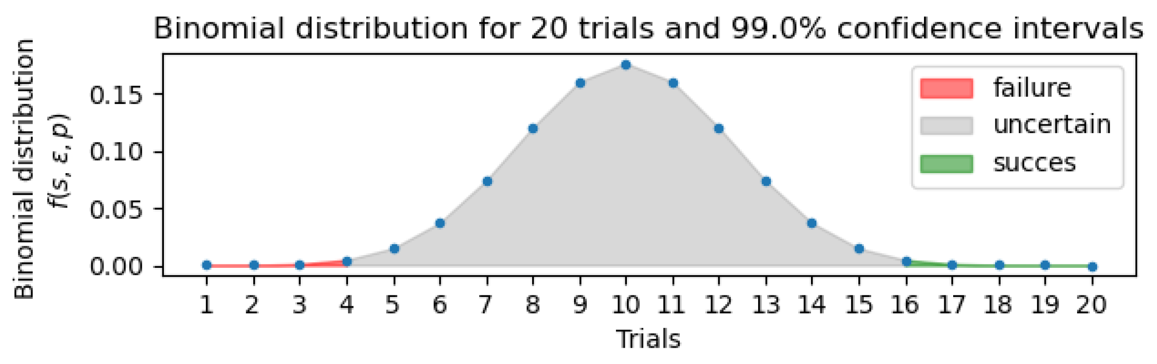
The total number of successful or unsuccessful performances, that each feature must reach, is driven by the binomial distribution as follows

$$f(s,ϵ,p)=\left(\genfrac{}{}{0pt}{}{ϵ}{s}\right)p^s{(1-p)}^{ϵ-s},$$

(3)

where $ϵ$ is the number of trials, $p\in \langle 0,1\rangle$ is the success probability for each trial and s is the total number of successful trials, so it defines confidence intervals as in the example in Figure 1. The number of successful performances of a feature, that is to be labeled as important for the data, is given only by the number of trials used. Successful features then create a new data set.

2.1.2. Multiscale False Neighbours Analysis (MSFNA)

The MSFNA is a technique used for the uncertainty evaluation of the state vector’s configuration as it evaluates the determinism for general input-output mapping $f\left(\mathbf{x}\right)=y$, i.e., the mapping $f\left(\right)$ between feature vectors $\mathbf{x}$ and corresponding outputs y [15]. Unlike common false neighbor analysis, which requires precise knowledge about the neighborhood radius, see [25,26], MSFNA uses a vector of several radii to scale the neighborhood condition. If $\mathbf{x}$ is the state vector of the system, then system output y is unambiguously determined by the input (state vector) $\mathbf{x}$ if the same input $\mathbf{x}$ results in different outputs y, the state vector is not complete and other features must be included, these states are then referred to as false neighbors (FN). Two states ${\mathbf{x}}_{\mathbf{1}}$, ${\mathbf{x}}_{\mathbf{2}}$ are FN if they meet the condition

$$if\parallel {\mathbf{x}}_{\mathbf{i}}-{\mathbf{x}}_{\mathbf{j}}\parallel <r_x\mathrm{AND}\parallel y_i-y_j\parallel >r_y\Rightarrow FN(i,j)=1;\mathrm{else}FN(i,j)=0,$$

(4)

where $r_x,r_y$ are absolute radii that define the condition of state similarity. Because optimal $r_x$ and $r_y$ is practically unknown, MSFNA utilizes the whole range of radii via heuristically designed vectors ${\mathbf{r}}_{\mathbf{x}}=[r_{x_1},r_{x_2},\cdots ,r_{x_{\alpha }}]$, ${\mathbf{r}}_{\mathbf{y}}=[r_{y_1},r_{y_2},\cdots ,r_{y_{\beta }}]$ assuming that the optimal radii lies within the ranges of radii of vectors ${\mathbf{r}}_{\mathbf{x}},{\mathbf{r}}_{\mathbf{y}}$. The Areal Cumulative False Neighbors $ACFN$ is computed according to

$$ACFN=\sum _{i=1}^N\sum _{j=i+1}^{N}FN(i,j),$$

(5)

where $ACFN$ is the sum of all false neighbors in the dataset that evaluates the uniqueness of the state vector configuration for each data point. The higher $ACFN$ gets, the less determinism, i.e., more false neighbors, is in the mapping of the designed feature vector configuration and prediction outputs.

To compare datasets with a different number of samples, we introduce the Relative ACFN ($RACFN$) that eliminates the dependence of $ACFN$ on the number of samples in the dataset by normalization via the total count of all neighbor pairs as follows

$$RACFN=\sum _{i=1}^N\sum _{j=i+1}^{N}FN(i,j){\displaystyle \frac{2}{N^2-2N}}\in \langle 0,1\rangle .$$

(6)

Apart from the number of samples, a dimension of the input matrix (state vector) is also a source of deceptive information arising from comparing euclidean distances of variously long state vectors against the same radii vectors ${\mathbf{r}}_{\mathbf{x}}$ and ${\mathbf{r}}_y$.

While (6) resolves the issue of various lenght of data, it still suffers from various lengths of feature vectors $n_x$ that BFSA can principally find for various datasets. Thus, we propose to resolve the non-unique feature-vector-length problem by compressing (column-wise) the matrix of state vectors $\mathbf{X}$ as in (1) using Principal Component Analysis (PCA) into a customized number of components $n_c$, i.e., the matrix $\mathbf{X}$ is compressed to a constant number of columns (new features), and the MSFNA is then evaluated for state vectors of the same length $n_c$. The PCA compression into $n_c$ features is applied as follows

$${\mathbf{X}}_{PCA}=\left[\begin{array}{c}{\mathbf{v}}_1\\ {\mathbf{v}}_2\\ ⋮\\ {\mathbf{v}}_{n_c}\end{array}\right]\mathbf{X},$$

(7)

where ${\mathbf{v}}_1,{\mathbf{v}}_2,\cdots ,{\mathbf{v}}_{n_c}$, are selected eigenvectors of covariance matrix ${\mathbf{C}}_X=\mathbf{X}{\mathbf{X}}^T$.

It can be noted, that the PCA compression prior $RACFN$ not only standardizes its results by unifying the feature vector length for various feature setups, but it also naturally increases the robustness of the MSFNA results as the PCA compression further removes unique features because $n_c$ of the most significant components are used for compression.

2.2. Data and Preprocessing

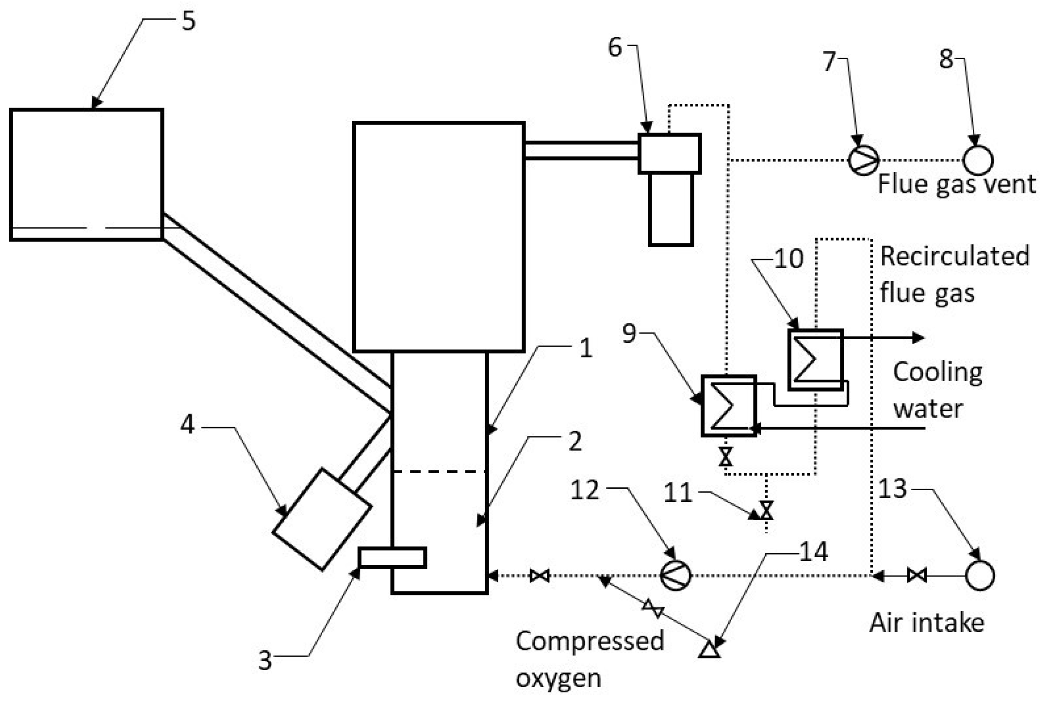
The experimental device is a 30 kW laboratory-scale oxy-fuel BFB combustor, the scheme is in the Figure 2. Sunflower pellets were used as biomass fuel.

The variables used for the analysis are listed in Table 1. As input variables $u_i$ are denoted features, that can be changed or indirectly influenced by the facility set-up. Output variables $y_i$ consist of the volumetric fractions of the flue gas components.

The experiment was realized by measuring four states of the oxy-fuel mode defined by secondary and primary oxygen flow ratios ${\displaystyle \frac{V_{O_2,sec}}{V_{O_2,prim}}}$. In each mode, there were 900 up to 1100 samples measured, as shown in

Table 2. Oxy-fuel modes measured during the experiment are defined by secondary and primary oxygen flow ratios.

mode 1	1109 samples with sampling period $\Delta T_s=2$ s	${\displaystyle \frac{V_{O_2,sec}}{V_{{\mathbf{O}}_2,prim}}}\approx 0$
mode 2	930 samples with sampling period $\Delta T_s=2$ s	${\displaystyle \frac{V_{O_2,sec}}{V_{O_2,prim}}}\approx 0.35$
mode 3	900 samples with sampling period $\Delta T_s=2$ s	${\displaystyle \frac{V_{O_2,sec}}{V_{O_2,prim}}}\approx 0.57$
mode 4	900 samples with sampling period $\Delta T_s=2$ s	${\displaystyle \frac{V_{O_2,sec}}{V_{O_2,prim}}}\approx 0.91$

. All oxy-fuel modes were measured at the same environmental conditions in one day.

Collected data were first checked for missing values and relevant data points were removed and replaced with the previous value. Data were resampled with four different sampling constants to compare the results: $\Delta T_1=5$ s, $\Delta T_2=10$ s, $\Delta T_3=15$ s and $\Delta T_4=25$ s. The new point is calculated as a mean value of previous points, which behaves as a simple smoothing filter. In the next step, the data were normalized using the Min-Max scaler as shown in (8) and (9).

$$X_{MinMax}\left(i\right)=X_S\left(i\right)(F{R}_{max}-F{R}_{min})+F{R}_{min}$$

(8)

$$X_S\left(i\right)={\displaystyle \frac{X\left(i\right)-min\left(X\right)}{max\left(X\right)-min\left(X\right)}}$$

(9)

$F{R}_{max}$ and $F{R}_{min}$ is the upper, respectively lower interval limit of the desired feature range; we used $\langle 0,1\rangle$. The last step is to design the state vector and matrix of states. The matrix of all state vectors $\mathbf{X}$ is defined as follows

$$\mathbf{X}=\left[\begin{array}{c}{\mathbf{x}}^T(k=1)\\ {\mathbf{x}}^T(k=2)\\ ⋮\\ {\mathbf{x}}^T(k=N)\end{array}\right],$$

(10)

where the full $\mathbf{X}$ before applying BFSNA for selecting optimal features is defined as follows.

$$\begin{array}{c}\hfill \mathbf{x}\left(k\right)=\left[{\mathbf{u}}_1\right[k-n_{u1}:k-1],{\mathbf{u}}_2[k-n_{u2}:k-1],\cdots \\ \hfill {\mathbf{y}}_1[k-n_{y1}:k-1]),{\mathbf{y}}_2[k-n_{y2}:k-1]),\cdots ],\end{array}$$

(11)

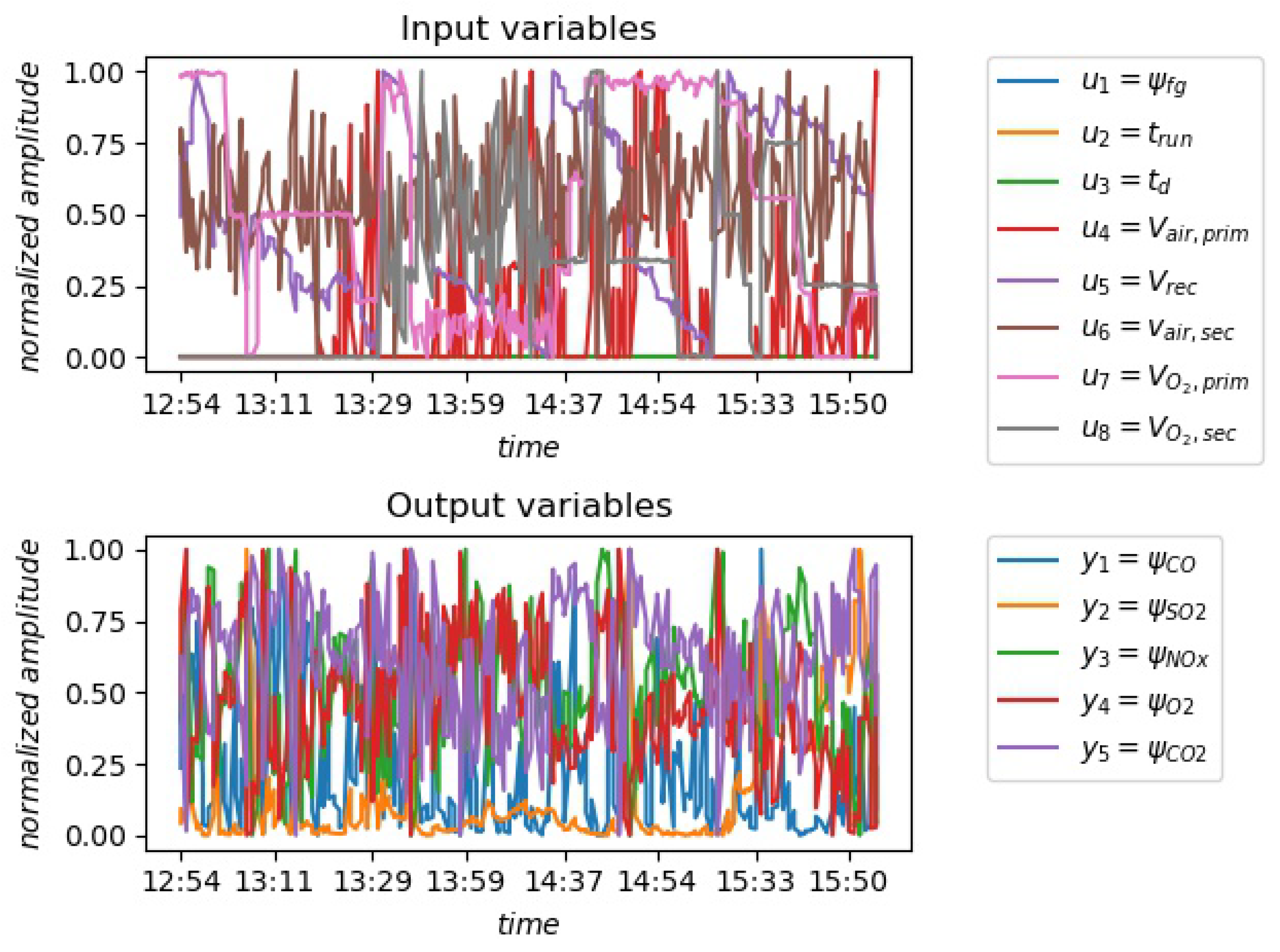
where the maximum number of step delays $n_{ui}$ and $n_{yj}$ are initialized heuristically, the meaning of input and output process variables is defined in Table 1. The snapshot of measured and min-max scored process variables $u_i$ and $y_j$ is shown in Figure 3.

For further details of the real device and the experimental setup, please kindly see [3,4,27].

2.3. Algorithm Complexity

The computational complexity of the BFSA is $O(n_x·N)$, where $n_x$ is the number of features and N is the number of samples [16]. The computational complexity of the Multiscale False neighbor analysis is $O(n_r·N)$, where $n_r=\alpha$ is the length of MSFNA absolute radii vector, see the text bellow Equation (4).

3. Experimental Analysis and Results

In this section, experimental analysis on artificial data and then on real data is shown for the algorithms described in Section 2.

3.1. Artificial Data

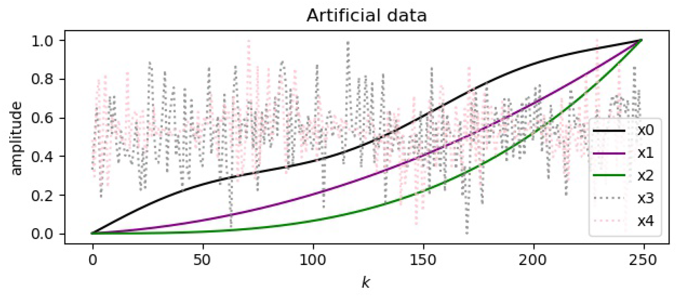
The first goal was to test the proposed algorithms on an artificial dataset of a simple MISO (multiple-input, single-output) system given by equations

$$\begin{array}{cc}\hfill & {\mathbf{X}}_{[k,:]}=[2k+sin\left(k\right),{(0.5·k)}^2+{\displaystyle \frac{k}{2}}-1,k^3+k^2],y\left(k\right)=\sum _{k=1}^3{\mathbf{X}}_{[k,i]},\hfill \\ \hfill & \mathrm{where}k=1,2,...N=250.\hfill \end{array}$$

(12)

Two additional variables ${\mathbf{X}}_{[:,3]}$ and ${\mathbf{X}}_{[:,4]}$ were added to test the BFSA, these columns are a combination of a sine, resp. cosine curve and white noise. The artificial data from (12) are plotted in Figure 4, where ${\mathbf{X}}_{[:,3]}$ and ${\mathbf{X}}_{[:,4]}$ are added to demonstrate that BFSA eliminates them and MSFNA detects more false neighbors via higher $RACFN$.

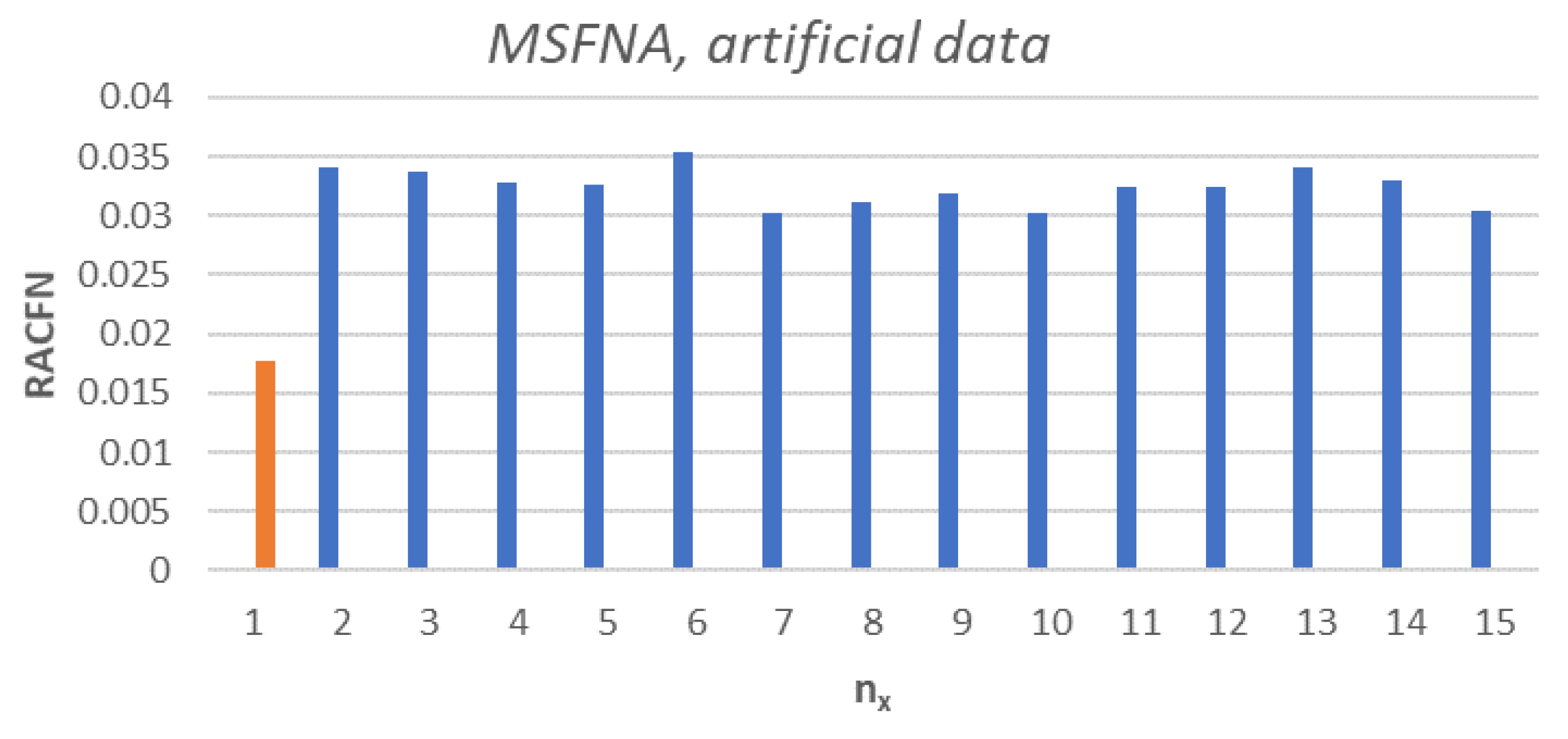
BFSA was applied on artificial data and features ${\mathbf{X}}_{[:,0]}$, ${\mathbf{X}}_{[:,1]}$ and ${\mathbf{X}}_{[:,2]}$ were correctly selected. In the next step, 15 combinations of possible input features were prepared as a combinations of 3 and 4 out of five possible features; $\left({\displaystyle \genfrac{}{}{0pt}{}{5}{3}}\right)+\left({\displaystyle \genfrac{}{}{0pt}{}{5}{4}}\right)=15$, compressed with PCA and $RACFN$s were calculated according to (6). The results are in Figure 5. The lowest value of $RACFN$ was determined for the input state vector proposed by BFSA $RACF{N}_{BFSA}=0.0178$, for the rest of the input vectors the $RACFN$ values lie in the interval $\langle 0.0309,0.036\rangle$. The input combination proposed by BFSA was proven to have the lowest count of $RACFN$ following the expectations. The result is in the Figure 5.

3.2. Experimental Data

For each output variable, a state vector $\mathbf{x}$ was designed. The maximum number of history samples of each feature was set to 15, as in Equation (11). Results for sampling periods $\Delta T=[5,10,15,25]$ s for each output variable are shown in

Table 3. Table of state vectors ${\mathbf{x}}_{\mathbf{i}}$ for outputs $y_i$ (listed in columns) proposed by Boruta Feature Selection Algorithm for sampling period $\Delta T_s=5$  s. Features $u_1$, $u_2$, $u_3$ were not picked by BFSA at all, $u_8$ is not chosen for $y_5$.

Variables		${\mathit{y}}_1={\mathit{\psi }}_{\mathbf{C}\mathbf{O}}$	${\mathit{y}}_2={\mathit{\psi }}_{\mathbf{S}{\mathbf{O}}_2}$	${\mathit{y}}_3={\mathit{\psi }}_{{\mathbf{NO}}_{\mathbf{x}}}$	${\mathit{y}}_4={\mathit{\psi }}_{{\mathbf{O}}_2}$	${\mathit{y}}_5={\mathit{\psi }}_{\mathbf{C}{\mathbf{O}}_2}$
Variables used for the input vector	$u_1={\psi }_{fg}$	-	-	-	-	-
	$u_2=t_{run}$	-	-	-	-	-
	$u_3=t_d$	-	-	-	-	-
	$u_4=V_{air,prim}$	4	7, 5	8, 2, 1	12, 10, 9, 8, 6, 5, 4	6
	$u_5=V_{rec}$	15, 14, …, 1	15, 12, 11, 9, 8, 5, 1	15, 14, …, 1	15, 14, 13, 11, 10, …, 1	15, 14, 12, 9, 7, 5, 3
	$u_6=v_{air,sec}$	15, 14, …, 1	15, 13, 9, 8, 7, 3	15, 14, …, 1	15, 14, …, 1	15, 12, 9, 8, 5, 4
	$u_7=V_{O_2,prim}$	15, 14, 13, 11, 9, 8, …, 1	15, 7, 6, 5, 3, 2, 1	15, 14, …, 1	15, 14, …, 1	15, 4, 3, 1
	$u_8=V_{O_2,sec}$	15, 13, 12, 11, 9, 8, 5, 3, 2, 1	10, 6	15, 14, …, 1	15, 14, …, 1	-
	$y_1={\psi }_{\mathrm{CO}}$	15, 14, 13, 10, 9, 7, 5, …, 1	15, 14, 12, …, 1	15, 14, …, 1	15, 14, …, 1	15, 12, 10, 9, 7, 1
	$y_2={\psi }_{{\mathrm{SO}}_2}$	15, 14, …, 1	15, 14, …, 1	15, 14, …, 1	15, 14, …, 1	14, 1
	$y_3={\psi }_{{\mathrm{NO}}_x}$	15, 14, …, 1	15, 14, …, 1	15, 14, …, 1	15, 14, …, 1	9, 8, 3, 2, 1
	$y_4={\psi }_{{\mathrm{O}}_2}$	15, 14, …, 1	8, 5, 4, 3, 2, 1	15, 14, …, 1	15, 14, …, 1	15, 13, 11, 8, 7, …, 1
	$y_5={\psi }_{{\mathrm{CO}}_2}$	15, 13, 12, 11, 7, 6, 5, …, 1	15, 13, 12, 10, 9, 8, 7, 5, 3, 2, 1	15, 14, …, 1	15, 14, …, 1	15, 14, 12, 11, 9, 7, 6, …, 1
$n_x$		121	84	138	141	54

,

Table 4. Table of state vectors ${\mathbf{x}}_{\mathbf{i}}$ for outputs $y_i$ (listed in columns) proposed by Boruta Feature Selection Algorithm for sampling period $\Delta T_s=10$  s. Features $u_1$, $u_2$, $u_3$ were not picked by BFSA at all, $u_4$ is not chosen for $y_5$ and $u_7$ is not included in state vector for $y_2$.

Variables		${\mathit{y}}_1={\mathit{\psi }}_{\mathbf{C}\mathbf{O}}$	${\mathit{y}}_2={\mathit{\psi }}_{\mathbf{S}{\mathbf{O}}_2}$	${\mathit{y}}_3={\mathit{\psi }}_{{\mathbf{NO}}_{\mathbf{x}}}$	${\mathit{y}}_4={\mathit{\psi }}_{{\mathbf{O}}_2}$	${\mathit{y}}_5={\mathit{\psi }}_{\mathbf{C}{\mathbf{O}}_2}$
Variables used for the input vector	$u_1={\psi }_{fg}$	-	-	-	-	-
	$u_2=t_{run}$	-	-	-	-	-
	$u_3=t_d$	-	-	-	-	-
	$u_4=V_{air,prim}$	3	3	11, 2, 1	12, 4	-
	$u_5=V_{rec}$	14, 13, …, 10, 5, 4, …, 1	15, 12, 11, 9, 8, 5, 1	15, 14, …, 1	15, 14, …1	13, 11, 10, 8, 4, 2, 1
	$u_6=v_{air,sec}$	15, 14, …, 1	9, 2	15, 14, …, 1	15, 14, …, 1	14, 13, …7, 3, 2
	$u_7=V_{O_2,prim}$	15, 14, …, 1	-	15, 14, …, 1	15, 14, …, 1	15, 12, 11, 9, 8, 6, 5, 3
	$u_8=V_{O_2,sec}$	15, 14, 10, 9, 6	14, 13	15, 14, …, 1	15, 14, …, 1	13, 10, 9, 6, 1
	$y_1={\psi }_{\mathrm{CO}}$	15, 14, …, 1	15, 5, 4, …, 1	15, 14, …, 1	15, 14, …, 1	15, 13, 12, …, 8, 5, 4, 2, 1
	$y_2={\psi }_{{\mathrm{SO}}_2}$	15, 14, …, 1	15, 14, 8, 7, …, 5, 2, 1	15, 14, …, 1	15, 14, …, 1	14, 12, 11, 10, 5, 3, 2, 1
	$y_3={\psi }_{{\mathrm{NO}}_x}$	15, 14, …, 1	13, 8, 7, 6, …, 3, 1	15, 14, …, 1	15, 14, …, 1	15, 14, 12, …, 7, 5, 3, 1
	$y_4={\psi }_{{\mathrm{O}}_2}$	15, 13, 12, 11, …, 5, 3, 2, 1	5, 4, 3, 2	15, 14, …, 1	15, 14, …, 1	15, …, 12, 10, …, 8, 5, …1
	$y_5={\psi }_{{\mathrm{CO}}_2}$	15, 14, …, 1	8, 7, …, 4, 2, 1	15, 14, …, 1	15, 14, …, 1	14, 13, 11, 10, 9, 8, 6, 4, 3, 2, 1
$n_x$		117	45	138	136	83

,

Table 5. Table of state vectors ${\mathbf{x}}_{\mathbf{i}}$ for outputs $y_i$ (listed in columns) proposed by Boruta Feature Selection Algorithm for sampling period $\Delta T_s=15$  s. Features $u_1$, $u_2$, $u_3$ were not picked by BFSA at all, $u_4$ is not chosen for $y_3$.

Variables		${\mathit{y}}_1={\mathit{\psi }}_{\mathbf{C}\mathbf{O}}$	${\mathit{y}}_2={\mathit{\psi }}_{\mathbf{S}{\mathbf{O}}_2}$	${\mathit{y}}_3={\mathit{\psi }}_{{\mathbf{NO}}_{\mathbf{x}}}$	${\mathit{y}}_4={\mathit{\psi }}_{{\mathbf{O}}_2}$	${\mathit{y}}_5={\mathit{\psi }}_{\mathbf{C}{\mathbf{O}}_2}$
Variables used for the input vector	$u_1={\psi }_{fg}$	-	-	-	-	-
	$u_2=t_{run}$	-	-	-	-	-
	$u_3=t_d$	-	-	-	-	-
	$u_4=V_{air,prim}$	15, 14, 10, 2	1	-	15, 7, 2	8, 7, 6
	$u_5=V_{rec}$	15, 14, …, 8, 6, 5, 1	14, 13, 11, 9, 8, …, 5, 3, 1	15, 14, 13, 9, 8, 6, 3, 2, 1	15, 14, …1	15, 14, …, 1
	$u_6=v_{air,sec}$	15, 14, …, 1	10, 8, 5	15, 14, 12, …, 1	15, 14, …, 1	15, 14, …, 1
	$u_7=V_{O_2,prim}$	15, 14, …, 1	15, 7, 5, 4, 2	15, 14, …, 1	15, 14, …, 1	15, 14, …, 1
	$u_8=V_{O_2,sec}$	15, 13, 10, 6, 4, 3, 1	14, 13, 12, 6	15, 14, …, 1	15, 14, …, 1	15, 14, …, 1
	$y_1={\psi }_{\mathrm{CO}}$	15, 14, …, 1	15, 13, 11, 10, 4, 2, 1	15, 14, …, 1	15, 14, …, 1	15, 14, …, 1
	$y_2={\psi }_{{\mathrm{SO}}_2}$	15, 14, …, 1	15, 14, …, 10, 8, …, 3, 1	15, 14, …, 1	15, 14, …, 1	15, 14, …, 1
	$y_3={\psi }_{{\mathrm{NO}}_x}$	15, 14, 12, 11, …, 11	15, 14, 13, 5, 3, 2, 1	15, 14, …, 1	15, 14, …, 1	15, 14, …, 1
	$y_4={\psi }_{{\mathrm{O}}_2}$	15, 14, 1	7, 6, …, 1	15, 14, …, 1	15, 14, …, 1	15, 14, …, 1
	$y_5={\psi }_{{\mathrm{CO}}_2}$	15, 14, …, 1	15, 12, 11, 6, 5, …1	15, 14, …, 1	15, 14, …, 1	15, 14, …, 1
$n_x$		126	67	127	138	138

and

Table 6. Table of state vectors ${\mathbf{x}}_{\mathbf{i}}$ for outputs $y_i$ (listed in columns) proposed by Boruta Feature Selection Algorithm for sampling period $\Delta T_s=25$  s. Features $u_1$, $u_2$, $u_3$ were not picked by BFSA at all, $u_4$ is not included in state vector for $y_5$.

Variables		${\mathit{y}}_1={\mathit{\psi }}_{\mathbf{C}\mathbf{O}}$	${\mathit{y}}_2={\mathit{\psi }}_{\mathbf{S}{\mathbf{O}}_2}$	${\mathit{y}}_3={\mathit{\psi }}_{{\mathbf{NO}}_{\mathbf{x}}}$	${\mathit{y}}_4={\mathit{\psi }}_{{\mathbf{O}}_2}$	${\mathit{y}}_5={\mathit{\psi }}_{\mathbf{C}{\mathbf{O}}_2}$
Variables used for the input vector	$u_1={\psi }_{fg}$	-	-	-	-	-
	$u_2=t_{run}$	-	-	-	-	-
	$u_3=t_d$	-	-	-	-	-
	$u_4=V_{air,prim}$	14, 10, 9, 2	9, 5, 1	10, 7, 21	4	-
	$u_5=V_{rec}$	15, 14, 12, 10, 9, 7, 6, 5, …, 1	14, 8, 6, 4, 3, 2, 1	15, 13, …, 4, 3, 1	15, 14, …11, 9, 8, …, 1	15, 13, …, 10, 8, …, 4, 2, 1
	$u_6=v_{air,sec}$	15, 14, …, 1	15, 10, 9	15, 14, …, 1	15, 14, …, 1	15, 14, …, 1
	$u_7=V_{O_2,prim}$	15, 14, …, 1	12, 11, …, 7	15, 14, 13, 12, 10, 9, …, 1	15, 14, …, 1	15, 14, …, 1
	$u_8=V_{O_2,sec}$	15, 14, …, 7, 8, 3	15, 14, 13, 11, 10, 9, 6	15, 14, 12, 9, 8, 7, …, 1	15, 14, …, 1	13, 10, 8, 7, 6, 4, 3, 2, 1
	$y_1={\psi }_{\mathrm{CO}}$	15, 14, …, 1	14, 13, …, 9, 6, 5, 1	15, 13, …, 10, 8, 7, …, 1	15, 14, …, 1	15, 14, …, 1
	$y_2={\psi }_{{\mathrm{SO}}_2}$	15, 14, …, 1	15, 14, 12, 11, …, 1	15, 14, …, 1	15, 14, …, 1	15, 14, …, 9, 7, 6, 4, …, 1
	$y_3={\psi }_{{\mathrm{NO}}_x}$	15, 14, …, 1	12, 11, 2, 1	15, 14, …, 1	15, 14, …, 1	15, 14, …, 1
	$y_4={\psi }_{{\mathrm{O}}_2}$	15, 14, …, 1	13, 10, 3, 2, 1	15, 14, …, 1	15, 14, …, 1	15, 14, …, 1
	$y_5={\psi }_{{\mathrm{CO}}_2}$	15, 14, …, 1	11, 10, 9, 3, 1	15, 14, …, 1	15, 14, …, 1	15, 14, …, 1
$n_x$		130	63	129	135	124

; one can notice, that variables $u_1={\psi }_{fg}$, $u_2=t_{run}$ and $u_3=t_d$ were not selected by BFSA as input features for any output variable $y_i$. Primary air flow $u_4=V_{air,prim}$ was used rather sparsely. The total number of state vector features is listed in the last row of Table 3, Table 4, Table 5 and Table 6.

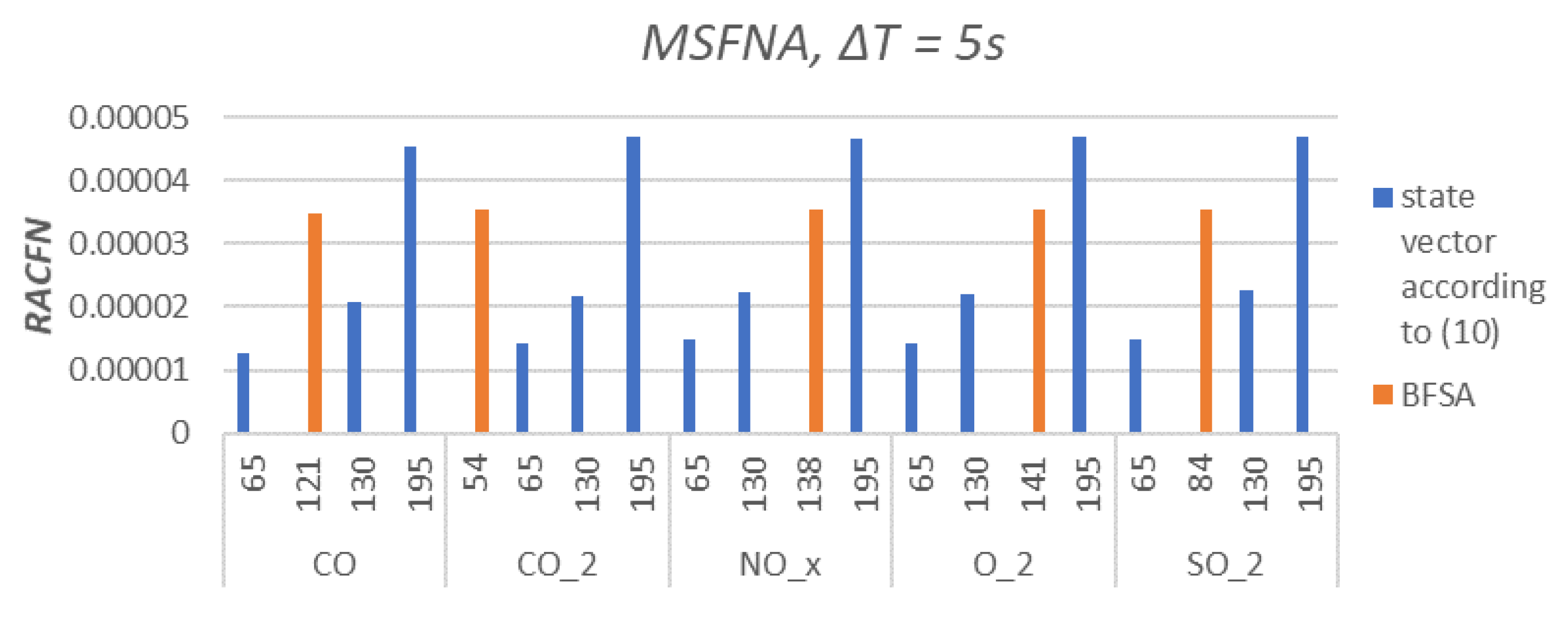
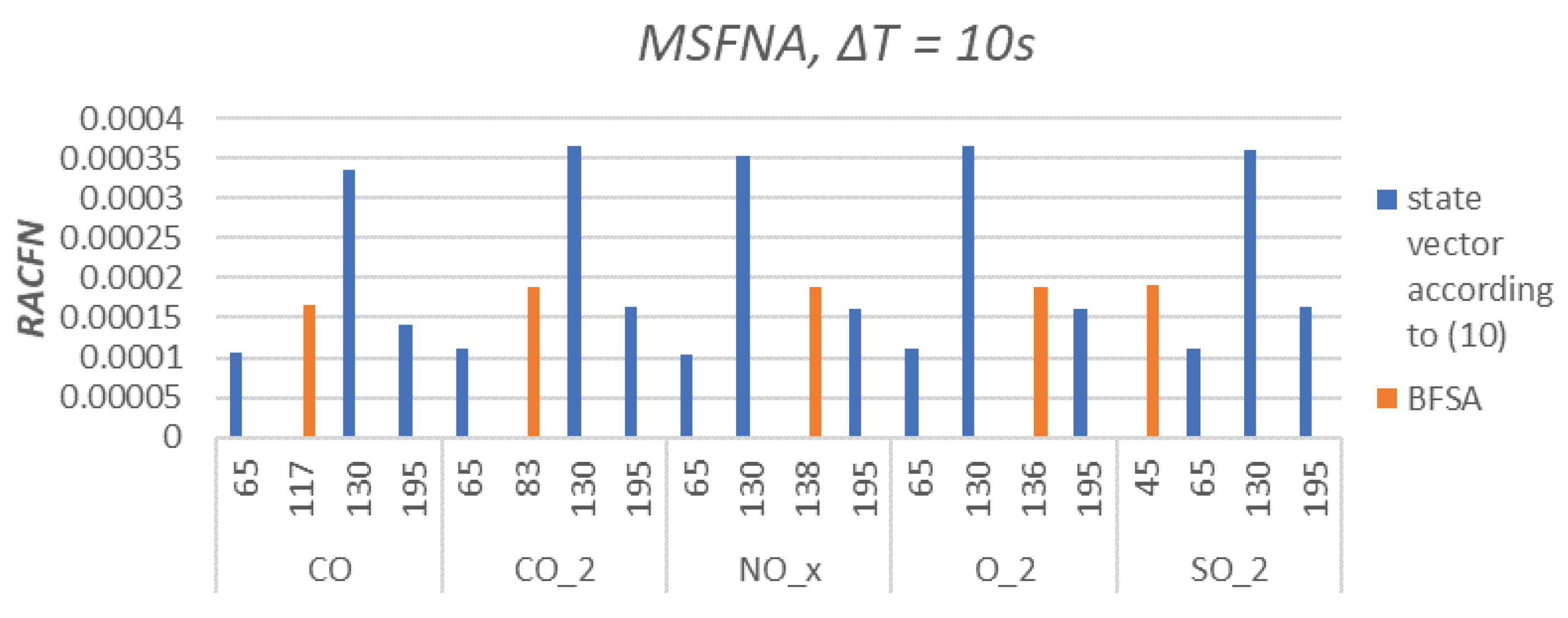
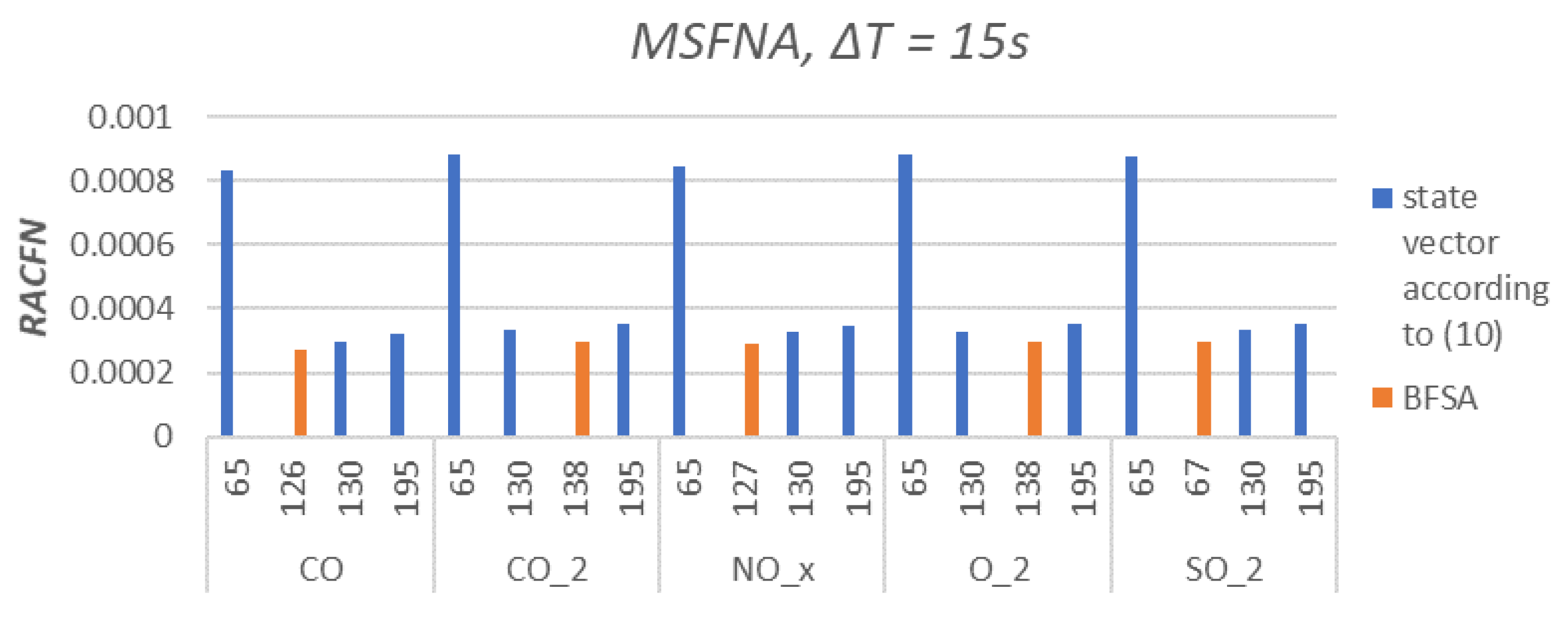
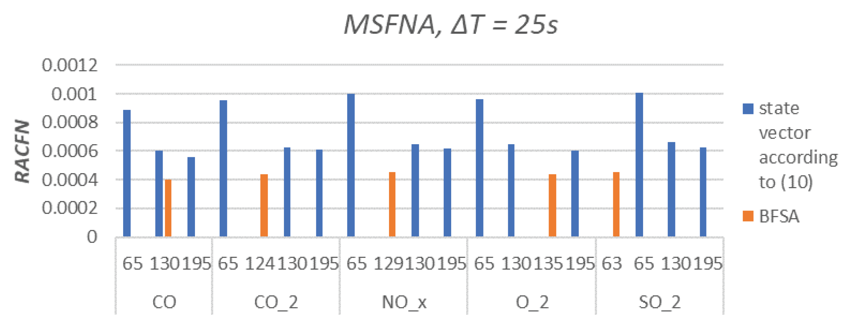
The Multiscale False Neighbours Analysis was performed with the same configuration for all samplings $\Delta T=[5,10,15,25]$ s. The step delays $n_{ui}$ and $n_{yj}$ were set as $[5,10,15]$, resulting to 3 state vector configurations with 3 different numbers of features; $n_x=[65,130,195]$. The fourth examined state vector is proposed by BFSA. Results are shown in Figure 6, Figure 7, Figure 8 and Figure 9. The $RACFN$ was chosen as a comparative quantity due to the ability to compare the examined state vectors’ data variance and graphically express the results.

4. Discussion

The major outcome of the feature selection by BFSA and its newly proposed validation of MSFNA is demonstrated via Figure 6, Figure 7, Figure 8 and Figure 9, where the different sampling periods ($\Delta T=[5,10,15,25]$ s) results in various levels of uncertainty ($RACFN$) between by-BFSA-designed feature vectors and process outputs. In Figure 6 and Figure 7, where the sampling is chosen faster (than in Figure 8 and Figure 9), the BFSA proposes such feature vector configuration that displays more uncertainty via $RACFN$ than other merely heuristic manual feature selections (Figure 6 and Figure 7). For longer sampling period (Figure 8 and Figure 9), the by-BSFNA-designed feature vectors already displays lowest uncertainty via $RACFN$ as well. Recall, that all $RACFN$ for all various feature vector configurations were evaluated by PCA compression of feature vectors to the equal length $n_c$ and that even naturally increases the robustness of the method as already discussed in Section 2.1.

Primary airflow $V_{air,prim}$, recirculation flow $V_{rec}$, and secondary air velocity $v_{air,sec}$ were selected by BFSA less often and differently for each sampling frequency that indicates their lower importance for emission prediction.

BFSA results, further validated by MSFNA, supports the assumption that the flue gas composition is strongly dependent on previous values of process output variables $y_i$, and this corresponds to the high complexity of the combustion dynamics where the measured values provide us only with a minimum necessary information about the actual process, so the emission prediction is still a challenge.

With a specific sampling frequency, a shape similarity can be observed across all output variables. It is the result of the strong sampling frequency dependence of the dynamic systems.

A minimum $RACFN$ was reached for the state vector designed by BFSA for longer sampling periods $\Delta T=15$ s and $\Delta T=25$ s. This finding corresponds to the assumptions of slower dynamical behavior of important phenomena in the real process for which we intend to predict the emissions (but in the following research as it would exceed the scope of this paper). It can be observed, that the uncertainty of the by-BFSA-designed features became improved for longer sampling of $\Delta T=15$ s (Figure 8), and it did not improve for longer samplings further (Figure 8 vs. Figure 9). Thus, the combination of BFSA and MFSNA not only selects features but also suggests a proper shortest sampling (for which $RACFN$ became the smallest out of the other non-BFSA feature designs).

5. Conclusions

The feature selection algorithm (BFSA) was studied for mapping between available measurements (features) and emissions (outputs) of bubbling fluidized bed oxy-fuel combustion data. Newly, the original uncertainty analysis (MFSNA) was extended (PCA & RACFN) and proposed to validate the BFSA in terms of uncertainty via false neighbors. The proposed technique is promising for the automatic configuration of feature vectors from measured data (for future prediction systems with machine learning). Furthermore, the combination of conventional BFSA with MSFNA appeared capable to clearly validate and propose a proper sampling period that is computationally difficult with standalone BFSA otherwise.

References

- Buhre, B.; Elliott, L.; Sheng, C.; Gupta, R.; Wall, T. Oxy-fuel combustion technology for coal-fired power generation. Prog. Energy Combust. Sci. 2005, 31, 283–307. [Google Scholar] [CrossRef]
- Toftegaard, M.B.; Brix, J.; Jensen, P.A.; Glarborg, P.; Jensen, A.D. Oxy-fuel combustion of solid fuels. Prog. Energy Combust. Sci. 2010, 36, 581–625. [Google Scholar] [CrossRef]
- Vodička, M.; Haugen, N.E.; Gruber, A.; Hrdlička, J. NOX formation in oxy-fuel combustion of lignite in a bubbling fluidized bed—Modelling and experimental verification. Int. J. Greenh. Gas Control 2018, 76, 208–214. [Google Scholar] [CrossRef]
- Vodička, M.; Hrdlička, J.; Skopec, P. Experimental study of the NOX reduction through the staged oxygen supply in the oxy-fuel combustion in a 30 kWth bubbling fluidized bed. Fuel 2021, 286, 119343. [Google Scholar] [CrossRef]
- Pitel, J.; Mižák, J. Computational intelligence and low cost sensors in biomass combustion process. In Proceedings of the 2013 IEEE Symposium on Computational Intelligence in Control and Automation (CICA), Singapore, 16–19 April 2013; pp. 181–184. [Google Scholar]
- Mižáková, J.; Pitel’, J.; Hošovský, A.; Kolarčík, M.; Ratnayake, M. Using Special Filter with Membership Function in Biomass Combustion Process Control. Appl. Sci. 2018, 8, 1279. [Google Scholar] [CrossRef] [Green Version]
- Tóthová, M.; Dubják, J. Using computational intelligence in biomass combustion control in medium-scale boilers. In Proceedings of the 2016 IEEE 14th International Symposium on Applied Machine Intelligence and Informatics (SAMI), Herl’any, Slovakia, 21–23 January 2016; pp. 81–85. [Google Scholar] [CrossRef]
- Li, N.; Lu, G.; Li, X.; Yan, Y. Prediction of NOx Emissions from a Biomass Fired Combustion Process Based on Flame Radical Imaging and Deep Learning Techniques. Combust. Sci. Technol. 2016, 188, 233–246. [Google Scholar] [CrossRef] [Green Version]
- Bai, X.; Lu, G.; Hossain, M.M.; Szuhánszki, J.; Daood, S.S.; Nimmo, W.; Yan, Y.; Pourkashanian, M. Multi-mode combustion process monitoring on a pulverised fuel combustion test facility based on flame imaging and random weight network techniques. Fuel 2017, 202, 656–664. [Google Scholar] [CrossRef] [Green Version]
- Korpela, T.M.; Björkqvist, T.K.; Lautala, P.A. Control Strategy for Small-Scale Wood Chip Combustion. IFAC Proc. Vol. 2009, 42, 119–124. [Google Scholar] [CrossRef]
- Smrekar, J.; Assadi, M.; Fast, M.; Kuštrin, I.; De, S. Development of artificial neural network model for a coal-fired boiler using real plant data. Energy 2009, 34, 144–152. [Google Scholar] [CrossRef]
- Leerbeck, K.; Bacher, P.; Junker, R.G.; Goranović, G.; Corradi, O.; Ebrahimy, R.; Tveit, A.; Madsen, H. Short-term forecasting of CO2 emission intensity in power grids by machine learning. Appl. Energy 2020, 277, 115527. [Google Scholar] [CrossRef]
- Reshef, D.N.; Reshef, Y.A.; Finucane, H.K.; Grossman, S.R.; McVean, G.; Turnbaugh, P.J.; Lander, E.S.; Mitzenmacher, M.; Sabeti, P.C. Detecting novel associations in large data sets. Science 2011, 334, 1518–1524. [Google Scholar] [CrossRef] [PubMed] [Green Version]
- Xie, P.; Gao, M.; Zhang, H.; Niu, Y.; Wang, X. Dynamic modeling for NOx emission sequence prediction of SCR system outlet based on sequence to sequence long short-term memory network. Energy 2020, 190, 116482. [Google Scholar] [CrossRef]
- Bukovsky, I.; Kinsner, W.; Maly, V.; Krehlik, K. Multiscale Analysis of False Neighbors for state space reconstruction of complicated systems. In Proceedings of the 2011 IEEE Workshop on Merging Fields of Computational Intelligence and Sensor Technology, Paris, France, 11–15 April 2011; pp. 65–72. [Google Scholar] [CrossRef]
- Kursa, M.B.; Rudnicki, W.R. Feature selection with the Boruta package. J. Stat. Softw. 2010, 36, 1–13. [Google Scholar] [CrossRef] [Green Version]
- Chandrashekar, G.; Sahin, F. A survey on feature selection methods. Comput. Electr. Eng. 2014, 40, 16–28. [Google Scholar] [CrossRef]
- Kumar, V.; Minz, S. Feature selection: A literature review. SmartCR 2014, 4, 211–229. [Google Scholar] [CrossRef]
- Yang, G.; Wang, Y.; Li, X. Prediction of the NOx emissions from thermal power plant using long-short term memory neural network. Energy 2020, 192, 116597. [Google Scholar] [CrossRef]
- Cuccu, G.; Danafar, S.; Cudré-Mauroux, P.; Gassner, M.; Bernero, S.; Kryszczuk, K. A data-driven approach to predict NOx-emissions of gas turbines. In Proceedings of the 2017 IEEE International Conference on Big Data (Big Data), Boston, MA, USA, 11–14 December 2017; pp. 1283–1288. [Google Scholar] [CrossRef]
- Adams, D.; Oh, D.H.; Kim, D.W.; Lee, C.H.; Oh, M. Prediction of SOx–NOx emission from a coal-fired CFB power plant with machine learning: Plant data learned by deep neural network and least square support vector machine. J. Clean. Prod. 2020, 270, 122310. [Google Scholar] [CrossRef]
- Shi, Y.; Zhong, W.; Chen, X.; Yu, A.; Li, J. Combustion optimization of ultra supercritical boiler based on artificial intelligence. Energy 2019, 170, 804–817. [Google Scholar] [CrossRef]
- Tuttle, J.F.; Blackburn, L.D.; Powell, K.M. On-line classification of coal combustion quality using nonlinear SVM for improved neural network NOx emission rate prediction. Comput. Chem. Eng. 2020, 141, 106990. [Google Scholar] [CrossRef]
- Kumar, S.S.; Shaikh, T. Empirical Evaluation of the Performance of Feature Selection Approaches on Random Forest. In Proceedings of the 2017 International Conference on Computer and Applications (ICCA), Doha, United Arab Emirates, 6–7 September 2017; pp. 227–231. [Google Scholar] [CrossRef]
- Abarbanel, H.D.I.; Kennel, M.B. Local false nearest neighbors and dynamical dimensions from observed chaotic data. Phys. Rev. E 1993, 47, 3057–3068. [Google Scholar] [CrossRef] [PubMed]
- Kennel, M.B.; Abarbanel, H.D.I. False neighbors and false strands: A reliable minimum embedding dimension algorithm. Phys. Rev. E 2002, 66, 026209. [Google Scholar] [CrossRef]
- Hrdlicka, J.; Skopec, P.; Opatril, J.; Dlouhy, T. Oxyfuel Combustion in a Bubbling Fluidized Bed Combustor. Energy Procedia 2016, 86, 116–123. [Google Scholar] [CrossRef] [Green Version]
Figure 1.
Example of a decision-making process for 20 trials according to Equation (3). Using 20 trials, the feature can be labeled as important if it scores higher than shadow features at least 16 times.
Figure 2.
Scheme of the 30 kWth BFB experimental, (1) fluidized bed region, (2) distributor of the fluidizing gas, (3) gas burner mount, (4) fluidized bed spillway, (5) fuel feeder, (6) cyclone separator, (7) flue gas fan, (8) flue gas vent, (9) and (10) water coolers, (11) condensate drain, (12) primary fan, (13) air-suck pipe, (14) vessels with oxygen, (sketch based on [3]).
Figure 3.
Snapshot of normalized, preprocessed data from one of the real experiments, are process input variables and are process output variables described in Table 1.
Figure 4.
Artificial data for testing, , and together create an output y, and are added to the system in order to test the feature selection and wrong feature elimination via BFSA and its validation via MSFNA.
Figure 5.
MSFNA on artificial data, the orange column corresponds with the input vector designed by BFSA, the rest of input combinations (blue) have a significantly higher number of FN, the results are consistent with the hypothesis.
Figure 6.
Relative Areal Cumulative False Neighbors for sampling periods s. Orange columns are state vectors proposed by BFSA and blue columns are state vectors created according to (11) with . Axis x represents the number of features for specified .
Figure 7.
Figure 8.
Figure 9.