Article

Vis-NIR Hyperspectral Imaging for Online Quality Evaluation during Food Processing: A Case Study of Hot Air Drying of Purple-Speckled Cocoyam (Colocasia esculenta (L.) Schott)

1
Department of Agricultural & Biosystems Engineering, Faculty of Organic Agricultural Sciences, University of Kassel, Nordbahnhof Str. 1a, 37213 Witzenhausen, Germany
2
Department of Environmental & Biosystems Engineering, School of Engineering, University of Nairobi, P.O. Box 30197, Nairobi 00100, Kenya
3
Department of Agricultural & Biosystems Engineering, School of Engineering & Technology, Kenyatta University, P.O. Box 43844, Nairobi 00100, Kenya
4
Department of Bioengineering of Horti-Viticultural Systems, Faculty of Horticulture, University of Agronomic Sciences and Veterinary Medicine of Bucharest, 59 Mărăști Boulevard, 011464 Bucharest, Romania
5
Department of Crop Sciences, Division of Quality of Plant Products, University of Göttingen, Carl-Sprengel-Weg 1, 37075 Göttingen, Germany
6
Leibniz Institute for Agricultural Engineering and Bioeconomy, Max-Eyth Allee 100, 14469 Potsdam, Germany
7
Albrecht Daniel Thaer-Institute of Agricultural and Horticultural Sciences, Humboldt Universität zu Berlin, Hinter der Reinhardtstr. 6–8, 10115 Berlin, Germany
*
Author to whom correspondence should be addressed.
Submission received: 19 September 2021 / Revised: 7 October 2021 / Accepted: 7 October 2021 / Published: 11 October 2021
(This article belongs to the Special Issue Progress in Food Processing)

Abstract

:
In this study, hyperspectral imaging (HSI) and chemometrics were implemented to develop prediction models for moisture, colour, chemical and structural attributes of purple-speckled cocoyam slices subjected to hot-air drying. Since HSI systems are costly and computationally demanding, the selection of a narrow band of wavelengths can enable the utilisation of simpler multispectral systems. In this study, 19 optimal wavelengths in the spectral range 400–1700 nm were selected using PLS-BETA and PLS-VIP feature selection methods. Prediction models for the studied quality attributes were developed from the 19 wavelengths. Excellent prediction performance (RMSEP < 2.0, r2P > 0.90, RPDP > 3.5) was obtained for MC, RR, VS and aw. Good prediction performance (RMSEP < 8.0, r2P = 0.70–0.90, RPDP > 2.0) was obtained for PC, BI, CIELAB b*, chroma, TFC, TAA and hue angle. Additionally, PPA and WI were also predicted successfully. An assessment of the agreement between predictions from the non-invasive hyperspectral imaging technique and experimental results from the routine laboratory methods established the potential of the HSI technique to replace or be used interchangeably with laboratory measurements. Additionally, a comparison of full-spectrum model results and the reduced models demonstrated the potential replacement of HSI with simpler imaging systems.

1. Introduction

Due to their wealth in vitamins, minerals, phytochemicals, carbohydrates and dietary fibre, fruits, vegetables and tubers are essential for a healthy human diet. Their deficiency can lead to chronic health conditions such as cancer, Alzheimer’s disease, diabetes osteoporosis, and heart disease, which contribute to about 3 percent of global deaths [1,2]. Even though strides have been made through the sustainable development goal (SDG) programmes to achieve food and nutritional security, various challenges and opportunities still abound [3]. Despite having access to some resources for food production and producing enough staples, small-scale farmers in rural areas remain the most food-insecure and undernourished in the world [4]. Additionally, with increasing urbanisation and growing incomes for urban dwellers, particularly in developing countries, the demand for conveniently available healthy foods, particularly processed fruits, vegetables and tubers is projected to increase [5,6].
Cocoyam (Colocasia esculenta) is a tuber crop cultivated and consumed in tropical and subtropical areas of the world [7,8]. Whereas it contributes to the carbohydrates and micronutrients consumed in these regions [9,10], its uptake and commercialization are hindered by seasonality and reduced shelf life in the fresh state due to the high moisture content of the tubers [7,11]. Various storage and preservation techniques for cocoyam include ventilated storage, refrigeration and storage in traditional low-cost structures [12]. However, hot-air drying is more popular because it is not only a method for preservation, but also for value-addition [11,13,14,15]. Hot-air drying is applied to reduce the amount of moisture in food materials to prevent the proliferation of spoilage microbes and to abate biochemical reactions. However, improper control of hot-air drying processes degrades the food quality in terms of poor visual appearance, poor rehydratability, loss of nutrients, destruction of bioactive compounds, and change in colour, texture and flavour [16]. Therefore, optimal control of the process is critical to not only preserve product quality, but also to reduce production costs [17,18].
Measurement of process attributes for quality control is a complex undertaking that often requires numerous resources including costly equipment, qualified personnel, and sufficient time [19]. Measurement of food quality attributes is customarily done physically in laboratories with manual feedback to the process. This not only makes continuous monitoring and automatic control difficult, but also leads to inconsistencies in the quality of measurements due to human bias and the fatigue associated with repeated measurements. As a consequence, changes in the properties of the product and process settings may go unnoticed, which results in loss of quality and ultimately negatively influences acceptability by consumers. Moreover, sample processing using laboratory methods is often destructive, and therefore, the samples are discarded after the tests [5]. Nonetheless, the optimal performance of any monitoring and control system is highly dependent on the quality and timeliness of such measurements [20]. This can be accomplished by transitioning from laboratory-based measurements to automated process monitoring and control. This would not only increase productivity, ensure flexibility, and achieve less downtime, but also guarantee the safety and quality of the food product [19,21,22].
Hyperspectral imaging (HSI) combined with chemometrics is a quickly evolving technique for real-time and non-destructive assessment of food quality attributes. The recent evolution of the technique is driven by improved instrumentation due to advances in computing speed, sensor technology and chemometric data analyses among others [23]. As opposed to conventional Vis-NIR spectroscopy, HSI provides spatial information of significance to particular product properties over a wide spectrum [24]. In the food industry, HSI has been applied to predict various quality attributes including fatty acid profiles in almonds and whole dried cocoa beans [25,26], soluble solids content and firmness in plums, apricots, kiwifruits and grapes [27,28], fibre content in pasta [29], microstructural changes in dry-cured pork [30], sugar content in potatoes [31], micronutrients in wheat [32], colour and acid content in hops [33], moisture content, colour, vitamin C, soluble solids content, firmness, shrinkage and rehydration ratio in apples [5,34,35], etc. In regard to cocoyam, NIR spectroscopy in the spectral range 350–2500 nm was applied to assess the content of starch, total sugars, cellulose, proteins, and minerals in 315 accessions of cocoyam for varietal selection and breeding [36]. Spectral information (1100–2500 nm) of cocoyam chips during deep frying was collected to predict changes in moisture content, fat content, colour and maximum breaking force [37].
To the best of our knowledge, information on the non-invasive measurement of quality attributes using the HSI technique during hot-air processing of purple-speckled cocoyam is documented. Additionally, for the first time, this study introduces the assessment of microstructural damage in plant material during hot-air drying using attributes including pore circularity (PC) and percentage pore area (PPA). Moreover, studies extending the HSI technique to multispectral applications during hot-air drying of food products are scarce. This study addresses this by reducing the wide spectrum related to HSI systems to a small subset of wavelengths that can be used with multispectral systems. The results of this study will support the development of smart dryers equipped with simple imaging systems for non-invasive quality assessment and process control. In conclusion, the objectives of this study were to (i) assess the feasibility of utilising HSI for non-invasive assessment of quality changes in purple-speckled cocoyam slices during hot-air drying, (ii) apply PLS-BETA and PLS-VIP to select the most optimal wavelengths, (iii) to correlate the selected optimal wavelengths with specific quality attributes of purple-speckled cocoyam slices during hot-air drying, (iv) to develop prediction models for the quality attributes from the selected optimal wavelengths using PLSR, and (v) to compare the agreement between the predictions from the PLSR models and results from laboratory experiments using method comparison techniques including Huber regression [38], Bland–Altman plots [39] and the Concordance Correlation Coefficient [40].

2. Materials and Methods

2.1. Materials and Sample Preparation

Mature cocoyam tubers (var. Colocasia esculenta (L.) Schott) were harvested in March 2020, inspected for blemishes, cleaned with a soft brush and cured in open sunlight for 8 h. Tubers without visual defects were selected for the experiments and stored in a laboratory refrigerator at 4 ± 1 °C. At the onset of experiments, the tubers were peeled, cleaned with distilled water and blotted with a soft absorbent towel. The first 25 mm of both ends of the tubers were sliced off due to possible differences in properties with the tuber mid-section. The flesh was then cut to a thickness of 4 mm and a diameter of 25 mm using a Graef Vivo V20EU bench slicer (Gebr. Graef GmbH & Co. KG, Arnsberg, Germany) and a core extractor, respectively.

2.2. Experimental Design and Drying Experiments

A completely randomised factorial experimental plan was prepared in the Design-Expert software version 11 (Stat-Ease Inc., Minneapolis, MN, USA). The input factors included drying temperature (40, 60 and 80 °C) and air velocity (2.0 ± 0.2, 3.0 ± 0.4 and 4.6 ± 0.7 m∙s−1). Drying experiments were conducted using an HT-mini convective dryer (Innotech-Ingenieursgesellschaft GmbH, Altdorf, Germany ±2 °C). The dryer design included a drying cabinet, a fan, a control panel, and perforated trays to hold the samples. The control panel provided a function to directly control the drying temperature and indirectly control the air velocity by varying the fan voltage. At the beginning of experiments, the dryer was preheated at the target settings for at least 30 min with all the trays inside the dryer to ensure a uniform initial environment. Experimental runs were then executed following the experimental plan until reaching the final moisture content of ~0.11 kgW/kgDM, which is within the ideal keeping conditions for the majority of roots and tubers [11,41]. During the experiments, samples were drawn from the drying cabinet every 30 min for measurement of moisture attributes (3 slices), colour attributes (3 slices), chemical attributes (9 slices) and structural attributes (3 slices). The slices collected for determination of some chemical and structural attributes were packed in vacuum bags using a LAVA V300 vacuum sealer (LANDIG Sondergerätebau, Bad Saulgau, Germany) and frozen at −28 °C until later analysis.

2.3. Quality Attributes

2.3.1. Moisture Attributes

Moisture content was determined following the procedure recommended by AOAC [42]. Samples were drawn from the drying cabinet every 30 min and weighed using a Sartorius E2000D digital balance, ±0.001 g (Sartorius AG, Göttingen, Germany). After each experiment, the samples were placed in a Memmert Oven Drier (Memmert GmbH, Büchenbach, Germany) to be dried at 105 °C for 24 h to determine the dry matter content (DM) as per AOAC (2000). Moisture content and moisture ratio were then calculated using Equations (1) and (2).
mc wb = M t M DM M t
where: mcwb = moisture content (wet basis), Mt = slice weight at time t, and MDM = dry matter mass.
MR = M t M e M i M e
where MR = moisture ratio, Mi = fresh slice weight and Me = equilibrium mass. The sample mass at equilibrium is negligible in comparison to Mt and Mi [43]. As such, Equation (3) can be re-written as follows [11];
MR = M t M i
Additionally, water activity (aw) was determined using a Novasina LabSwift water activity meter (Novasina AG, Lachen, Switzerland). Measurements were taken in a controlled environment inside a VCL 400 climate chamber (Vötsch Industrietechnik GmBH, Reiskirchen-Lindenstruth, Germany) with the relative humidity setting at zero and temperature at 25 °C.

2.3.2. Colour Attributes

The colour of slices was evaluated during the drying process with a Konica Minolta CR400 colourimeter (Minolta, Osaka, Japan), which was calibrated against a white standard tile before each measurement. Colour values were determined as the average of measurements taken on three slices with three measurements per slice. The colour attributes were then expressed in the CIELAB colour space [44]. The colour attributes were computed using Equations (4)–(8) [11];
BI = 100 · x 0 . 31 0 . 172
x = a * + 1 . 75 L * 5 . 645 L * + a * 3 . 012 b *
WI = 100 100 L t + a * + b * 1 2
C * = a * 2 + b * 2 1 2
h o = arctan b * a *
where BI = browning index, WI = whiteness index, C* = chroma, ho = hue angle, L* = lightness (0 = dark, 100 = light), a* = greenness/redness (−/+ = green/red), and b* = blueness/yellowness (−/+ = blue/yellow).

2.3.3. Chemical Attributes

The samples preserved for chemical analysis were freeze-dried in a Christ Epsilon 2-40 freeze dryer (Martin Christ Gefriertrocknungsanlagen GmbH, Osterode am Harz, Germany) at −85 °C for 96 h. The freeze-dried slices were then pulverized into a fine powder using a Jankel & Kunkel A10 mill (Jankel & Kunkel K.G., Staufen im Breisgau, Germany). The milled samples were then transferred into airtight PVC containers for storage before chemical extraction. The extraction process involved mixing about 0.3 g of each sample in 10 mL of 80% v/v ethanol, then vigorously shaking the mixture with a vortex mixer until the mixture was fully homogenized. The mixture was then immediately centrifugated using a Megafuge 16 (Thermo Fisher Scientific, Waltham, MA, USA) for 10 min at 5000 RPM. The supernatant was carefully collected using a micropipette with disposable tips into a 10 mL round bottom flask and the difference made up to the mark with 80% v/v ethanol. The mixture was then transferred into an airtight container and stored in a freezer at −20 °C.
The total phenolic content (TPC) was assayed using the Folin–Ciocalteu method [45]. The reagents utilised included sodium hydroxide (0.5 mol/L), gallic acid monohydrate (2.643 g/L) and the Folin–Ciocalteu reagent. A standard solution of C7H8O6 (concentration range 0–59.7 μg/mL) was prepared. The analytical mixture of 2.6 mL of deionised water, 300 μL of ethanolic extract, 1 mL of NaOH and 100 μL of the Folin–Ciocalteu reagent in a capped centrifuge tube was vigorously shaken with an Assistent Reamix 2789 vortex mixer (Glaswarenfabrik Karl Hecht GmbH, Sondheim vor der Rhön, Germany) and incubated in a GFL 1083 water bath (Lauda Wobser GmbH, Lauda-Königshofen, Germany) at 37 °C for 15 min. After incubation, the tubes were cooled down in water and the samples were transferred into cuvettes. A control sample containing 2.9 mL of deionised water and 1.1 mL of 80% v/v ethanol was prepared to blank the spectrophotometer before readings. The TPC concentration was then measured using an Agilent 8453 UV-Vis spectrophotometer (Agilent Technologies, Waldbronn, Germany) at a wavelength of 735.8 nm. Table 1 provides the absorbance spectra of the gallic acid monohydrate working solution at different concentrations. The results were recorded in μg of gallic acid per g of dry matter (μg GA/gDM).
The total flavonoid content (TFC) was analysed using the aluminium chloride method [46]. The reagents used included aluminium chloride (2% w/v), sodium acetate (1 M) and quercetin-3-glucoside (125 mg/L in methanol). A standard solution of C21H20O12 (concentration range 0–60 mg/L) was prepared. The analytical mixture of 750 μL of the ethanolic extract, 375 μL of AlCl3 and 375 μL of CH3COONa in a capped centrifuge tube was shaken vigorously with a vortex mixer and incubated in a water bath at room temperature for 30 min. A control sample containing 750 μL of 80% v/v ethanol, 375 μL of deionised water and 375 μL of CH3COONa was prepared to blank the spectrophotometer before readings. TFC was then determined using the spectrophotometer at a wavelength of 425 nm. Table 2 provides the absorbance spectra of the quercetin-3-glucoside working solution at different concentrations. The results were recorded in mg per g of dry matter (mg/gDM).
The 2,2-Diphenyl-1-picrylhydrazyl (DPPH) assay was utilised to analyse the sample for total antioxidant activity (TAA) [47]. First, 7.88 mg of DPPH was dissolved in 100 μL of methanol and incubated for 2 h at ambient temperature in a dark enclosure. A mixture of 0.3 mL ethanolic extract and 1.2 mL of the DPPH solution in a capped centrifuge tube was shaken vigorously using a vortex mixer. The contents were then incubated at ambient temperature in a dark enclosure for 30 min. A control sample consisting of 1.5 mL of 80% v/v ethanol was used to blank the spectrophotometer before readings. The absorbance of the samples was then read at a wavelength of 515 nm. TAA was then computed using Equation (9). TAA was then expressed as percent radical scavenging activity (RSA).
TAA   ( % ) = A C A o A C   ×   100
where: TAA = total antioxidant capacity (% RSA), AC = absorbance of control solution at 515 nm, and Ao = absorbance of sample at 515 nm.

2.3.4. Structural Attributes

(a)
Rehydration ratio
Rehydration experiments were undertaken to determine the degree of moisture re-uptake at the onset and the conclusion of each drying run [11]. The experiments involved dipping 3 slices into a GFL 1083 water bath (Lauda Wobser GmBH, Lauda-Königshofen, Germany) with water temperature at 95 °C for 10 min. The weight of fresh slices and the slices after rehydration was determined with a Sartorius Excellence E2000D digital balance, ±0.001 (Sartorius AG, Göttingen, Germany). The rehydration ratio was then computed using Equation (10) [11];
RR = W i W r
where: RR = rehydration ratio (-), Wi = slice weight after drying (g), and Wr = slice weight after rehydration (g).
(b)
Volumetric shrinkage
Volumetric shrinkage was determined using a combination of the pixel counting method [48] physical measurements. The thickness of the slices was measured using a Blueline micrometre screw gauge (Vogel GmbH, Kevelaer, Germany) at four different points on the slices and the average was computed. Volumetric shrinkage was then computed using Equation (11);
V s = V t V o = A t · h t A o · h o
where: Vs = volumetric shrinkage, Vo = initial volume of slice, Vt = slice volume at time t, Ao = initial slice top surface area (pix), At = slice top surface area at time t (pix), ho = initial thickness of slice (mm), and ht = thickness of slice at time t.
(c)
Structural morphology
Samples drawn during drying for the analysis of structural morphology were studied using Scanning Electron Microscopy (SEM) to extract morphological information including the total area occupied by pores and the circularity of the pores. The samples were freeze dried using a Christ Epsilon 2–40 freeze dryer (Martin Christ Gefriertrocknungsanlagen GmbH, Osterode am Harz, Germany) at −85 °C for 96 h. SEM was undertaken following the procedure proposed by [49]. The samples were dipped into liquid nitrogen for 5 s to prevent structural changes during specimen preparation then attached to a double-sided adhesive carbon tab mounted on the SEM stubs [49]. The samples were then coated with gold-palladium and studied under a Phillips xT Scanning Electron Microscope (Philips Export BV, Eindhoven, Netherlands) operating at a low vacuum, a voltage of 5 kV, a pressure of 100 Pa and 200 times magnification [49].
The Fiji software was utilised to pre-process the SEM images and to extract morphological information [50]. Pre-processing operations applied to improve the quality of the images included scaling, thresholding, filtering, de-speckling and water-shedding. The raw images were converted into 8-bit images where each pixel was assigned a grey-scale value in the range 0–255. The Li Minimum Cross-Entropy threshold-based segmentation method was found suitable to categorize pixels as foreground or background pixels depending on their grey-scale values [51]. Pores in the material were presented in white and the solid cocoyam material in black in the binary images. Complete pores with an area equal to or greater than 400 μm2 were counted, while those crossing the edges of the region of interest were ignored. The circularity of the pores was calculated using Equation (12). Circularity values approaching 0 indicated elongated polygons, while those approaching 1.0 indicated a perfect circle [52].
PPC = 4 π area perimeter 2

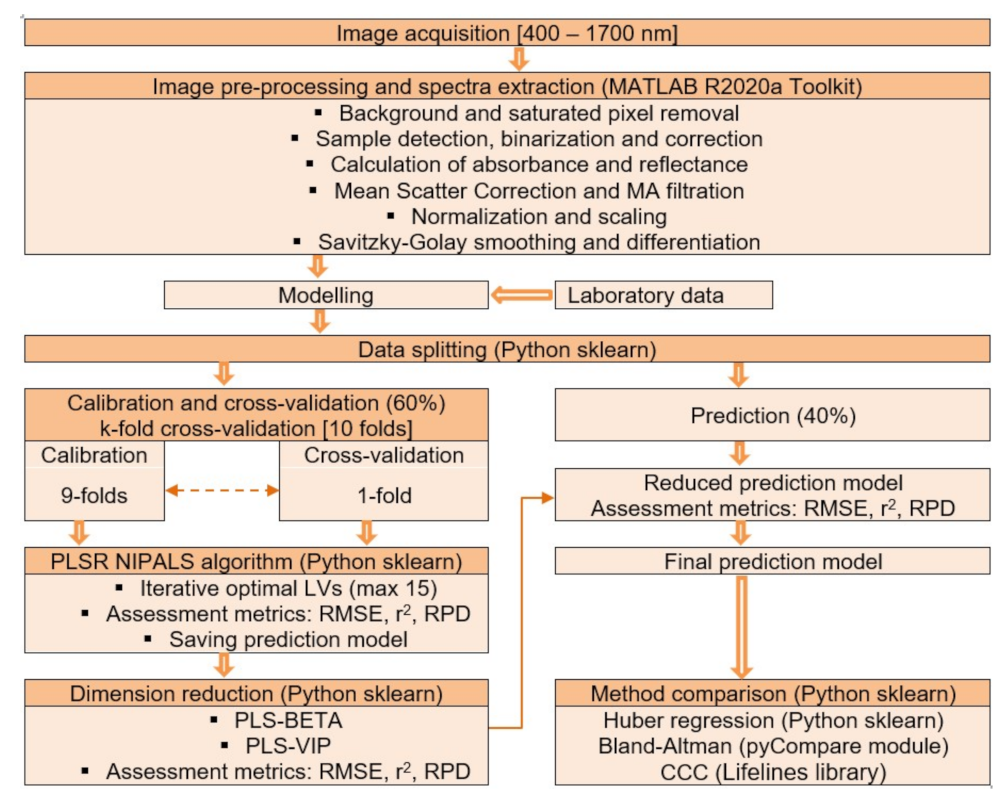
2.4. Hyperspectral Image Acquisition, Processing and Analysis

2.4.1. Overview

Figure 1 summarises the process followed in data acquisition, processing and prediction model development.

2.4.2. HSI Acquisition

This study utilised a combination of two HSI systems operating in the visible to the near-infrared region with a combined range of 400–1700 nm. The first camera system operated in the range 400–1010 nm with a sampling rate of 1.5 nm. The system consisted of a V10E PFD camera (Specim Spectral Imaging Ltd., Oulu, Finland) stocked with a 35 mm Xenoplan 1.9/35 lens (Jos. Schneider Optische Werke GmbH, Bad Kreuznach, Germany) operating on a linear translation stage (Specim Spectral Imaging Ltd., Oulu, Finland). The translation platform was illuminated with a combination of 105 W halogen lamps and 56 W LED lamps fixed at an angle of 45°. The second camera system worked in the range of 937–1700 nm with a sampling rate of 3.5 nm. It consisted of an FX17 camera (Specim Spectral Imaging Ltd., Oulu, Finland) stocked with a 17.5 mm OLET 17.5 N f/2.1 lens (Specim Spectral Imaging Ltd., Oulu, Finland) with a motorised linear translation stage (Specim Spectral Imaging Ltd., Oulu, Finland). The translation platform was illuminated with 120 W halogen lights fixed at 45°. In both systems, a standard white tile with a length and width of 200 mm and 25 mm was placed alongside the samples. A dark image was also taken with the camera shutter closed.

2.4.3. HSI Processing

The hyperspectral images were processed using a code programmed in the MATLAB® software version R2020a (MathWorks, Natick, MA, USA). Processing was done using a MSI Aegis RS computer (Micro-Star International Co., Taipei, Taiwan). The processing computer was stocked with a 32G Random Access Memory and an octa-core processor (Intel Core i9 9900K 8 × 3.6 GHz). The image channels were automatically searched to select the one providing the best contrast between foreground objects and the backgrounds. The selected channel was then binarized where values of 0 and 1 were assigned to the backgrounds and foreground objects, respectively. The binary image mask was then applied to segment the objects from the backgrounds. The white and dark references captured during image acquisition were used to correct the non-uniformity of light and sensor noise. Equation (13) was applied in the correction process,
R R = R S R D R w R D   ×   100
where: RR = adjusted relative reflectance of the image, RS = relative reflectance of the original images, RW = relative reflectance of the white reference, and RD = relative reflectance of the dark reference.
The average relative reflectance spectra for all samples were then calculated. The wavelengths below 425 nm and above 1700 nm were discarded owing to their low signal–noise ratio. The spectra were then improved by applying the Moving Average (MA) filter, Multiplicative Scatter Correction (MSC), the first derivative of reflectance (d.(R)) and the second derivative of reflectance (d2.(R)). The MA filter was utilised to smooth the spectra and MSC to eliminate multiplicative and additive scattering. The Savitzky–Golay smoothing and differentiation filter with a second-order polynomial was applied to calculate smoothed d.(R) and d2.(R). The improved spectra were then subjected to multivariate modelling.

2.4.4. Multivariate Modelling

PLSR was implemented in the scikit-learn library of Python Software to correlate the spectral data to the quality attributes [53]. First, the data were transformed to follow a Gaussian distribution by fitting a standard scaler feature-wise. This involved subtracting the mean value of spectra from each value then dividing it with the standard deviation of the whole dataset. The data was then randomly split into a 60 percent training set and a 40 percent hold-out testing set. The training dataset was utilised for calibration and cross-validation while the independent testing dataset was utilised to evaluate the prediction power of the developed PLSR models. A k-fold cross-validation scheme with 10 folds was used on the training dataset where 9 folds were used for calibration and one-fold for testing in each iteration. The optimal number of PLS components were found using the non-linear iterative partial least squares (NIPALS) algorithm in scikit-learn using a maximum of 15 Latent Variables (LVs). The optimal PLS components were selected based on returning the lowest Root Mean Squared Error (RMSEC) and the highest coefficient of determination (r2C) and Residual Prediction Deviation (RPDC) using Equations (14)–(16). RPD provides an assessment of the relative predictive performance of the model. Values of RPD less than 1.5 indicates the model is unacceptable, RPD between 1.5–2.0 indicate the ability of the model to differentiate low values from high values, 2.0–2.5 indicates rough estimations are possible, 2.5–3.0 corresponds to good prediction accuracy while values above 3.0 indicate excellent prediction accuracy [54,55]. An RPD value above 10 indicates the model is equivalent to the standard method [56].
RMSE C / RMSE P = i = 1 N y i y i ^ 2 N
where: RMSEC = Root Mean Squared Error for calibration, RMSEP = Root Mean Squared Error for prediction, yi = observations, y i ^ = predictions, and N = number of data points.
r C 2 / r P 2 = 1   y i y i ^ 2 y i y ¯ 2
where: r C 2 = coefficient of determination for calibration, and r P 2 = coefficient of determination for prediction.
RPD C / RPD P = y i y i ^ 2 N 2
where: RPD C = Residual Prediction Deviation for calibration, and RPD P = Residual Prediction Deviation for prediction.

2.4.5. Selection of Optimal Wavelengths

HSI obtains highly dimensional data because the spatial and spectral details collected provide plenty of information about the target objects. The data is also highly correlated, making it very complex. Dimensionality reduction is therefore necessary before any valuable information can be extracted using multivariate statistical techniques. Dimensionality reduction removes redundant information, reduces computation requirements and improves the prediction performance of the resulting models [57]. Popular dimensionality reduction or feature selection methods include Univariate feature selection (UFS), Genetic algorithms (GA), Random Forests (RF), Recursive Feature Elimination (RFE), Partial Least Squares-BETA (PLS-BETA) and Variable importance ranking (VIP) among others [58,59,60,61]. An assortment of machine learning techniques for predictive modelling after feature selection is also available. The PLSR method is more popular for linear predictive modelling due to its relative simplicity, ability to model multiple variables and robustness in the presence of noise and missing data [62,63].
(a)
PLS-BETA
The maximum number of wavelengths for the prediction of the quality parameters were identified by filtering and sequential elimination of wavelengths based on the PLS ß-coefficients using Python code. The process involved building the prediction model with the complete spectrum using the optimal PLS components. The PLS ß-coefficients were arranged in order of increasing magnitude, and the features with the lowest absolute ß-coefficients were then removed one at a time while evaluating the RMSEC, r2C and RPDC values returned by the PLS model without the single wavelengths. The process was iterated until the removal of a single wavelength either degraded or no longer improved the statistical quality measures. New PLS models were then developed with the reduced set of wavelengths and the model predictions were compared to the held-out testing data. RMSEP, r2P and RPDP were computed to evaluate the performance of the new models.
(b)
PLS-VIP
Partial Least Square Variable Importance in Projection (PLS-VIP) was utilised to select a set of influential wavelengths from the developed PLS models [64]. PLS-VIP plots were used to visualize the relationship between features and PLS-VIP scores for each quality attribute under consideration. The PLS-VIP scores were calculated using Equation (17) in Python using the find_peaks and peak_prominences functions in the SciPy library [65]. Wavelengths with PLS-VIP scores above 1.0 were considered as the most influential on the particular quality attributes.
VIP j = a = 1 A SS a 2 · W aj / W a 2 1 N · a = 1 A SS T
where VIPj = PLS-VIP score of the jth wavelength, A = number of PLS components, SSa = variance accounted by the ath component, SST = total variance accounted by all components, and N = total number of features [66].

2.5. Validation and Method Comparison

Comparison of a new method of measuring a particular phenomenon to standard methods to assess their comparability and compatibility is common in the applied sciences. This is because pertinent system variables are often measured with error [67]. Therefore, the comparison process applies statistical methods to quantify the error in the new method and to explain its influence on predictions [68]. Classical comparison methods utilise indices such as the coefficient of determination (r2) and the correlation coefficient (r). However, utilisation of these indices has been criticized because they measure the degree of linear association, but not the actual agreement between two datasets [69,70]. Nonetheless, techniques utilising robust estimates of regression coefficients, robust metrics of prediction accuracy, concordance indices and analysis of differences are more appropriate in method comparison studies to assess the degree of agreement [5,68,71,72]. In this study, the following methods were applied to assess the agreement between predictions and observations.

2.5.1. Huber Regression

Huber loss was applied to robustly fit a linear regression model between the observations and predictions. The coefficients of the regression equation were utilised to judge the agreement between the observations and predictions. A perfect agreement would give a slope of 1 and an intercept of 0 [73]. The student’s t-test was applied to test with the hypotheses that the slope is 1 and the intercept is 0 and that their values lie within the 95 percent confidence interval. The coefficients of the regression equation were obtained using the Huber Regressor class in the scikit-learn library of the Python software [53]. To ensure maximum robustness to outliers and asymptotic efficiency of at least 95 percent, an adaptive value of the tuning constant in the Huber estimator’s t function was evaluated using the method discussed in [74] and Equation (18). The Mean Absolute Deviation of the residuals was used as the robust measure of spread instead of the Standard Deviation.
k = 1 . 345   ×   MAD y i y i ^ 0 . 6745
where: k = tuning constant, MAD = Mean Absolute Deviation, yi = observations, and y i ^ = predictions.

2.5.2. Bland–Altman Plots and Analysis

Bland–Altman plots were utilised to visually inspect the strength of agreement between the observations and predictions [39]. The pyCompare module in the Python software was applied to build the plots [75]. The strength of agreement was established by examining the plots for the number of differences lying within or outside the 95 percent Limits of Agreement (LOA), the absence of bias and the lack of noticeable trends in the scatter plot of differences.

2.5.3. Concordance Correlation Coefficient

The Concordance Correlation Coefficient (CCC) was applied to evaluate the agreement between the observations and predictions and to gauge the reproducibility of the results [70]. CCC was determined using Equation (19), using the Lifelines library in the Python software [76]. The interpretation of the value of CCC varies widely depending on the field of application. The values of CCC ranging 0.7–1.0 indicate good agreement, 0.4–0.7 moderate agreement and 0–0.4 poor agreement [77].
CCC = 2 S xy S x 2 + S y 2 + x ¯ y ¯ 2
where: Sx = variance in observations, Sy = variance in predictions, Sxy = covariance between observations and predictions, x ¯ = mean of observations, and y ¯ = mean of predictions.

2.5.4. Statistical Analysis

The computations, multivariate analyses and statistical analysis performed in this study rely on the assumption that the datasets depict a Gaussian distribution, and that the variance is uniform. Therefore, various statistical checks were performed to ensure that these basic assumptions were obeyed. The D’Agostino–Pearson test was performed to test for Gaussian distributions and histograms were also constructed to visually confirm the same [78]. Homogeneity of variance was confirmed by performing Levene’s test [79]. Finally, the student’s t-test was also performed as an initial gauge for the existence of bias between observations and predictions. The SciPy library in the Python software was utilised to perform all statistical analyses [65].

3. Results

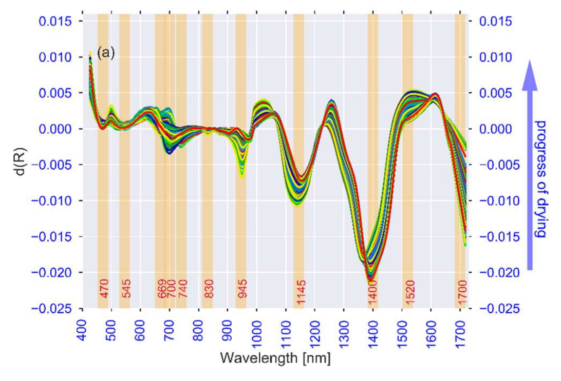
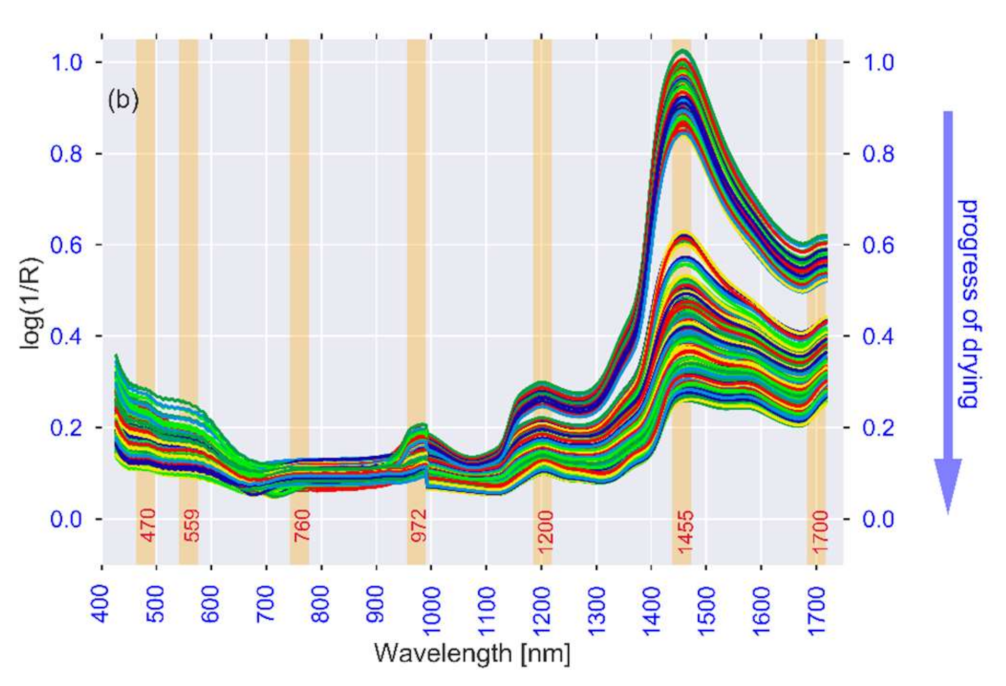
3.1. Spectral Analysis

The spectral signatures of cocoyam slices over the ranges 400–1700 nm during hot-air drying are shown in Figure 2. The spectral information was observed to be greater in the range above 900 nm as compared to 400–900 nm. Generally, absorbance was lower in the lower end of the spectrum, but higher in the upper end with the highest values in the region 1200–1700 nm. Previous studies have shown that certain wavelengths have special importance in providing information on the physicochemical properties of the material under consideration. For purple-speckled cocoyam, these wavelengths are highlighted and labelled in Figure 2. Shift or drifts in peaks of the expected locations of informative wavelengths occurred possibly due to spatial variations in chemical composition, drying temperature changes, interactions of hydrogen bonds with sample components and possibly minor changes in the alignment of the material surface to the optical path of the cameras [80,81,82].
There is a small but perceptible absorption peak in the vicinity of ~760 nm, which is associated with the stretching of the third overtone of O-H and the fourth overtone of CH in its vicinity [33,83]. The region 950–1000 nm is significant in the prediction of moisture content in tubers [84,85]. This region coincides with the absorbance peak at 972 nm and the dip at 945 nm in the first derivative plot. In the second overtone region, the absorbance at 1200 nm and 1400 nm has also been associated with moisture content in biological materials [86]. Independent analysis revealed relatively higher values of absorbance at these bands in the initial stages of drying (i.e., at 0, 30 and 60 min) because the high moisture content caused higher light absorption as a result of stretching and bending of O-H bonds within the water molecules [33,85,87]. The total amount of moisture in a food matrix can be segregated into free and bound water. Free water supports food spoilage microorganisms and chemical reactions [88,89]. It, therefore, is a significant indicator of food quality and is manifested in the matrix as water activity [90]. The informative bands for free water are in the vicinity of ∼950 and ∼1398 [91]. This is consistent with the troughs of the first derivative plots in the same region. These bands could be useful for the prediction of water activity.
Bound water is unavailable for chemical reactions, but has a great influence on material structure. The migration of bound water within a material causes the formation of pores, cellular shrinkage and collapse of cellular walls thereby contributing to overall structural deformation [92,93]. The rehydration ratio is commonly utilised as a structural deformation assessment index during food drying [11,94,95,96]. In this study, the change in slice structural attributes including rehydratability, volumetric shrinkage, percentage pore area and pore circularity are, therefore, theorized to be influenced by the removal of bound water. Wavebands in the vicinity of 1174 nm, 1454 nm, and 1496 nm are reported to depict absorption of water with a higher number of strong hydrogen bonds, which is representative of bound water [91,97,98]. These bounds could be significant in the prediction of material structural behaviour.
The flesh of a cocoyam tuber contains about 12.2–36.0 g of carbohydrates per 100 g of dry matter, where 70–80 percent is starch [99,100]. Sugars are another component of carbohydrates with sucrose as the largest proportion [100]. The absorption bands related to starch and sugars are in the third overtone of the stretching of O-H bonds in the region 720–920 nm and C-H bonds at 750–910 nm [101,102,103]. The wavelengths in the vicinity of 1593 nm have also been applied in predicting sucrose in sugar beet [104]. However, sucrose forms strong hydrogen bonds with water, and therefore its informative bands overlap with the region of strong moisture absorbance, thereby making them difficult to visualize [102,105].
Cocoyam contains various bioactive compounds with a strong antioxidant potential, a characteristic that makes it attractive as an important food and ethnomedical item [9,106]. Phenolic compounds in cocoyam, in particular, anthocyanins, contribute to red, purple or blue pigmentation in various accessions [107,108,109,110,111]. The fresh material utilised in this study contained an average of TPC 3.94 ± 0.68 µg GA/g DM and TFC 1.57 ± 0.14 mg/g DM. These compounds, when combined with the rich vitamin content, contribute to the high antioxidant activity of the tuber [106,112]. In this study, the average TAA was 77.4 ± 4.99% RSA. A decline in the prominence of absorption peaks in the region 700–1000 nm due to variation in the concentration of polyphenolic compounds as drying progressed was observed [33]. Phenolic compounds are also reported to absorb at bands in the spectral ranges 1415–1512 nm and 1650–1750 nm [113,114,115,116]. The dip in the first derivative plot at 1700 nm and the absorbance peak observed at the same wavelength are indicative of a possible informative band for bioactive compounds.
The colour exuded by materials is a result of the interaction of light at certain wavelengths with chemical compounds and organic materials [117]. Bands in the range of 400–700 nm are important in the assessment of colour [118,119]. Respectively, the blue, green and red components of colour are detectable in the regions 400–500 nm, 500–600 nm and 600–700 nm [120]. However, these colours tend to overlap at certain wavelengths, thereby exuding a wide range of mid-tones and colour differences [121]. An increase in the browning index and a decline in the whiteness index of cocoyam slices with the progress of hot-air drying due to enzymatic browning was reported [11]. This could explain the absorbance peaks at 545 nm and 559 nm attributable to the relative contribution of green and red pigments in the brown compounds. Moreover, previous studies have correlated the absorbance peaks in the region 516–560 nm to anthocyanins in plant materials [122,123].

3.2. Development of Calibration Models

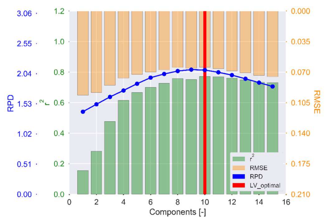
3.2.1. Selection of Optimal PLS Latent Variables

In this study, the optimal number of LVs was considered to be the value where no statistically significant improvement in RMSE, r2 and RPD was observed when additional LVs were included in the model during cross-validation. The maximum number of LVs tested was 15. As shown in Figure 3, the red line shows that the optimal number of LVs for TFC.
Table 3 provides the performance metrics of the PLSR models at calibration and prediction. As it can be seen in Table 3, better model performance was obtained from the spectra pre-processed by applying Multiplicative Scatter Correction to reflectance spectra followed by applying the second derivative. Moreover, the optimal latent variables obtained ranged from 5 for PC to 15 for WI and RR.

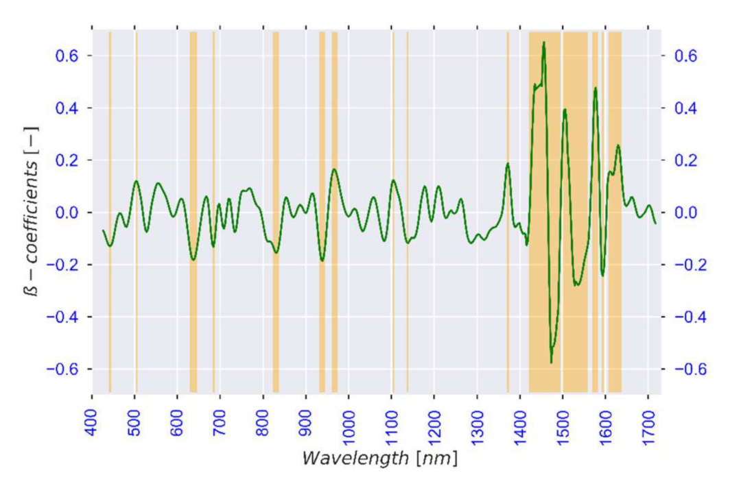
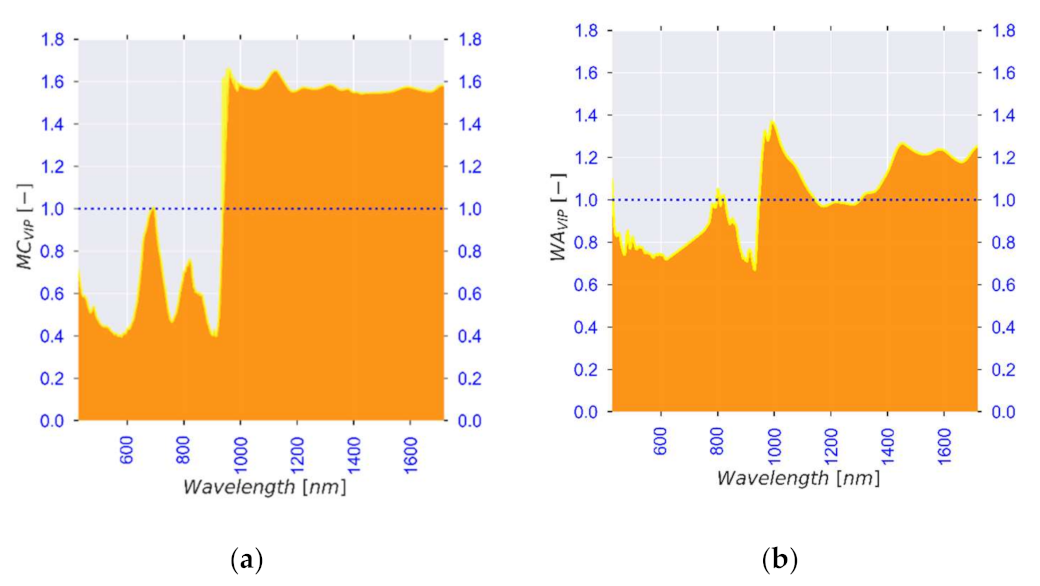
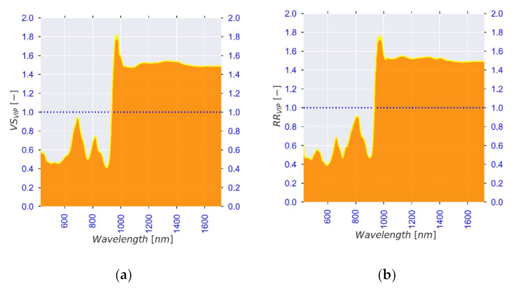
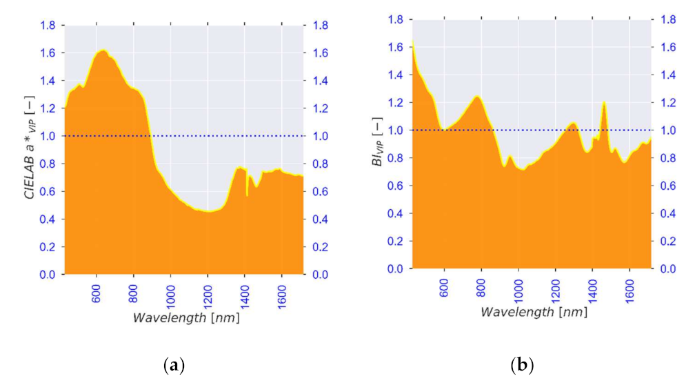
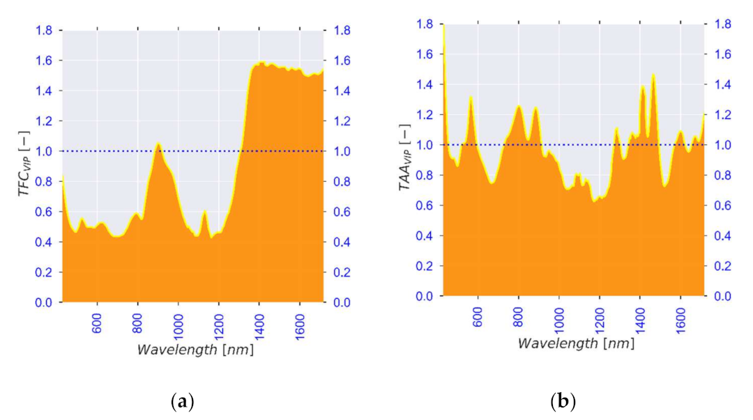
3.2.2. Selection of Optimal Wavelengths

Analysis of data from a large number of hypercubes is computationally demanding. Therefore, the selection of a subset of wavelengths with high information value and reduced co-linearity and redundancy is important [124]. PLS-BETA and PLS-VIP are some of the most frequently used methods for feature selection because of their simple implementation, less computational demand, and having few parameters requiring tuning [60,125,126]. Additionally, the two techniques have been reported to be complementary [127]. In the PLS-BETA method, PLSR coefficients are ranked and the ones with the largest contribution to the model are selected [101,125,127]. Figure 4 highlights the features selected using the PLS-BETA method for MC. It can be observed from the magnitudes of the ß-coefficients that the most influential features are in the upper end of the spectrum in the range 1380–1650 nm.
The PLS-VIP method assigns VIP scores to each variable based on the weighted sum of squares of the PLS weights. The ‘greater than one’ rule is the standard utilised as the cut-off value to decide the features to be selected [64,128]. Figure 5, Figure 6, Figure 7 and Figure 8 present PLS-VIP plots of the quality attributes under consideration.
In Figure 5a, wavelength bands in the region of 700–760 nm and 951–999 nm have high VIP scores owing to the third overtone of O-H indicating their importance in predicting moisture content. The viability of these bands is well documented in previous studies [5,84,85,86]. As shown in Figure 5b, the region 962–990 nm exhibits a high VIP score peak (approx. 1.4) for water activity. A broad peak is also exhibited at 1448 nm, but with a relatively lower VIP score. This could be attributed to the huge quantity of free water in the material, especially in the initial stages of drying. With free water as a proxy indicator of water activity [90,91], the bands in these regions are viable for future prediction of water activity. On the other hand, VIP scores for volumetric shrinkage and rehydration ratio are presented in Figure 6a,b, respectively. The wavebands at 977 nm and 975 nm for volumetric shrinkage and rehydration ratio, respectively, were found to depict VIP scores higher than in moisture content and water activity in the same region. Similarly, high VIP scores were obtained for percentage pore area and pore circularity. The application of heat during drying diminished the amount of free water in the cocoyam matrix. With less free water available, further application of heat mobilized bound water into extracellular space thereby enabling its removal through the normal channels. Structural attributes could therefore be envisaged as proxies for the combined free water and bound water. Since bound water does not exert vapour pressure, it theoretically has zero influence on water activity [129]. However, small but perceptible peaks are depicted in the vicinity of 1150 nm and 1400 nm. Previous studies have associated the regions with bound water [91,92,93,97,98,130]. The bands in these regions could therefore be utilised to predict structural changes in cocoyam material during drying.
Figure 7a,b present the VIP scores of CIELAB a* and browning index (BI). As shown in Figure 7a, the dominant wavebands for CIELAB a* are in the vicinity of 520 nm and 624–640 nm, which is consistent with the findings of [120]. This could be attributed to the purple-red pigmentation of speckles on the cocoyam slices associated with anthocyanins [122,123]. While the importance of this waveband region in the detection of chlorophyll in green plant material is well documented [33,131], limited information is available on its utility in predicting red pigments in plant materials. Red and green form an opponent colour pair in the CIELAB colour space [132]. The high VIP scores in the region 520 nm and 624–640 nm could therefore indicate the utility of these wavelengths in the detection of anthocyanins in cocoyam. Figure 7b presents the VIP scores for the BI, the most prominent peak is exhibited at 775 nm in the fourth overtone zone of C-H. This peak could be indicative of the degradation of phenolic compounds to brown coloured compounds like malvidin 3-O-glucoside as a result of drying [11,133,134].
Figure 8a,b present the VIP scores of the total flavonoid content and total antioxidant activity, respectively. The informative waveband for TFC is at 903 nm in the third overtone zone of C-H. Smaller peaks in the VIP plot were observed at 1407–1600 nm in the first overtone combination zone for C-H. These regions have been associated with phenolic compounds [113,114,115]. Phenolic compounds combined with the vitamins in cocoyam tubers contribute to its high antioxidant activity [106,112]. The peaks in the TFC VIP plot also appear in the TAA VIP plot at similar wavebands as shown in Figure 8a,b. However, the TAA VIP plot has additional peaks at 522, 558, 802, 884, 1273, 1360, 1412, 1465 and 1600 nm. These peaks could be related to other bioactive compounds not quantified in this study.

3.3. Modelling and Method Comparison

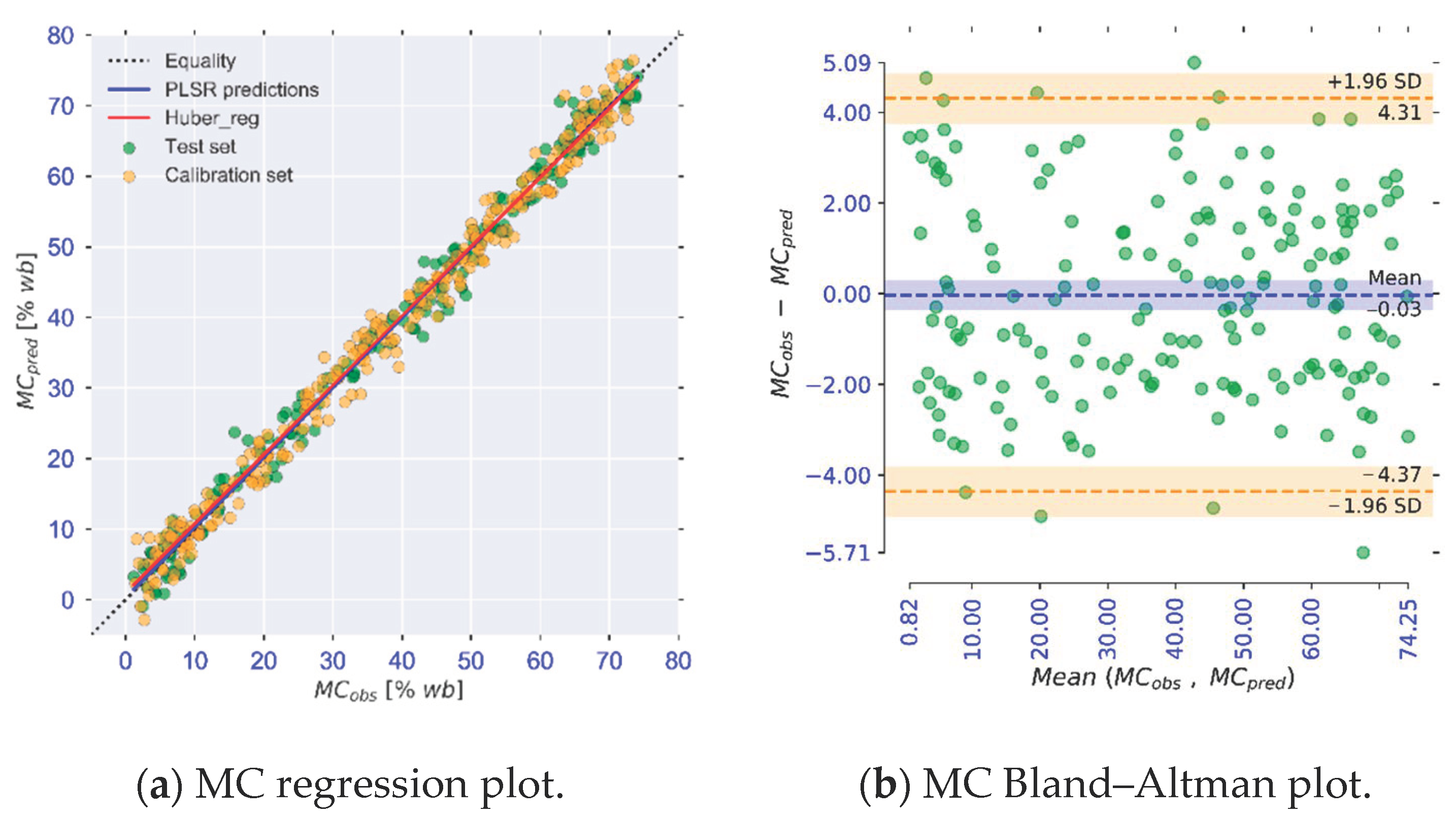
3.3.1. Moisture Attributes

The fresh purple-speckled cocoyam material utilised in this had an initial moisture content of 68.8 ± 3.0% on the wet-basis. The water activity of the material measured at 25 °C was 0.976 ± 0.002. MC, aw and MR were adequately modelled with 13, 11 and 10 LVs, respectively. Good prediction performance was observed with low values of RMSEP (i.e., 1.978, 0.030, 0.065), high values of r2P (i.e., 0.99, 0.99, 0.92) and high values of RPDP (i.e., 11.2, 10.8, 3.5). Considering these values of RPDP and the recommendation of [56], the models for MC and MR are equivalent to their standard methods of measurement. Table 4 provides the method comparison metrics for MC, aw and MR while Figure 9a,b provide the regression plot and Bland–Altman plot, respectively, for MC.
The results reveal a high degree of agreement between the predictions and observations for MC and MR with values of regression coefficients (ß0 and ß1) not significantly different from 0 and 1, respectively. The Bland–Altman plot shows few points outside the LOA, but the confidence interval for the mean difference includes zero. However, the degree of agreement of predictions and observations for aw was inadequate as deduced from the slope and intercept of the regression line and CCC. This is because the PLSR model slightly underestimated water activity values at the initial stages of drying and considerably overestimated water activity as the drying process approached the end, thereby diminishing the slope and increasing the value of the intercept of the regression line.

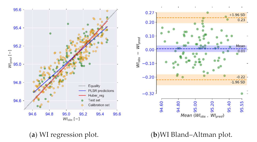
3.3.2. Colour Attributes

In this study, the CIELAB colour values (L*, a* and b*) of fresh cocoyam slices were measured to be 86.28 ± 1.18, 1.69 ± 0.39 and 7.51 ± 0.70, respectively. The best model results for colour attributes were obtained using absorbance spectra for BI and chroma, the first derivative of reflectance for CIELAB L*, b*, WI and hue and the second derivative of reflectance for CIELAB a*. The best prediction performance was obtained for BI (RMSEPP = 0.491, r2P = 0.78, RPDP = 2.4). Table 5 provides the method comparison metrics for colour attributes while Figure 10 provides the regression plot and Bland–Altman plot for WI.
The metrics reveal a good agreement between predictions and observations for BI, WI, CIELAB b*, chroma and hue angle. This was corroborated by the Bland–Altman plots which exhibited only a few differences outside the 95 percent limits of agreement. Further, irregular patterns associated with heteroscedasticity were absent and the confidence intervals for the respective mean differences included zero.

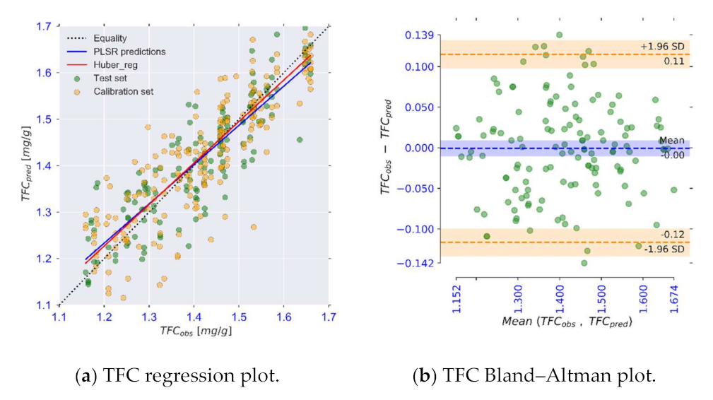
3.3.3. Chemical Attributes

The cocoyam tubers utilised in this study contained on average, TPC of 4.75 ± 0.23 µg GA/gDM, TFC of 1.43 ± 0.04 mg/g DM and TAA of 80.98 ± 0.18% RSA. TAA, TFC and TPC were adequately modelled using the second derivative of reflectance with 13, 12 and 9 LVs, respectively. A good prediction performance was obtained for TAA (RMSEPP = 7.600, r2P = 0.69, RPDP = 1.9) and TFC (RMSEPP = 0.063, r2P = 0.76, RPDP = 2.2). However, poor prediction performance was obtained for TPC (RMSEPP = 0.280, r2P = 0.45, RPDP =1.3). This could be as a result of unevenness in TPC assessed at each point of drying leading to an underfitting problem. A similar finding was reported by [34].
As provided in Table 6, good agreement between the predictions and observations was observed for TAA and TFC with regression coefficients (ß0 and ß1) not significantly different from 0 and 1, respectively. Satisfactory values of CCC were also obtained for the two attributes. This is confirmed by the method comparison metrics in Table 6 and Figure 11. The Bland–Altman plots for TAA and TFC also indicated good agreement between the methods, with a few outlying differences, absence of a noticeable trend in the scattered differences and the line of zero mean difference lies within the confidence interval of the mean difference.

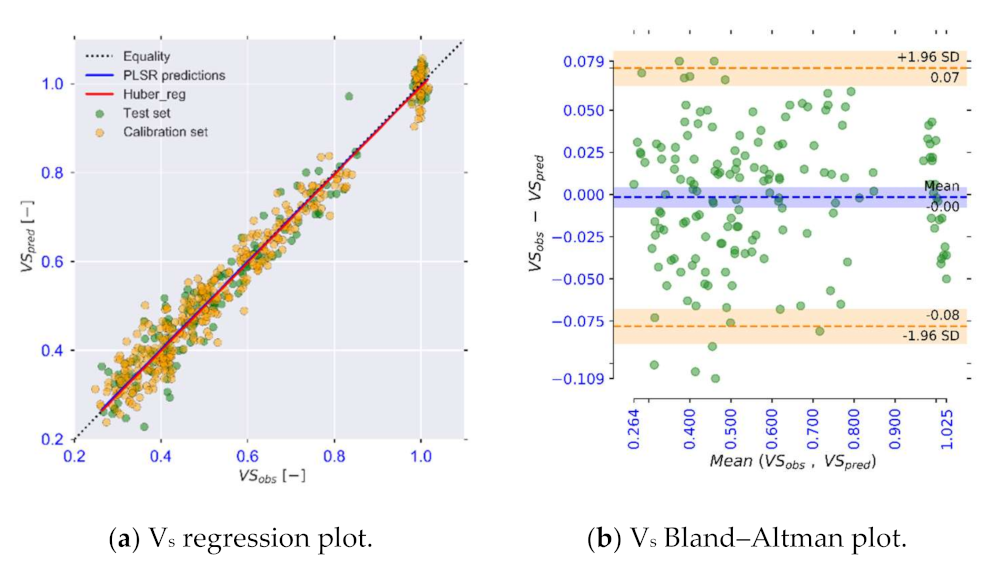
3.3.4. Structural Attributes

The best model results for volumetric shrinkage (Vs), percentage pore area (PPA) and pore circularity (PC) were acquired from the second derivative of reflectance data with 9, 9 and 5 LVs, respectively, while the rehydration ratio was best modelled using the first derivative of reflectance with 15 LVs. Excellent prediction performance was obtained for Vs (RMSEPP = 0.042, r2P = 0.96, RPDP = 5.2), RR (RMSEPP = 0.021, r2P = 0.98, RPDP = 7.0) and pore circularity (RMSEPP = 0.022, r2P = 0.84, RPDP = 2.4), while a good performance was obtained for PPA (RMSEPP = 2.347, r2P = 0.64, RPDP = 1.8). Table 7 provides the method comparison metrics for the structural attributes under consideration. The regression coefficients (ß0 and ß1) obtained for all the attributes were not significantly different from 0 and 1, respectively.
It can be observed from Figure 12 that the regression line for Vs overlaps the identity line. This is corroborated by the values of CCC and the Bland–Altman plots for the attributes. The Bland–Altman plot shows only a few points lie outside the 95% limits of agreement, the absence of a trend in the scattered points and that the confidence interval for the mean difference includes zero.

4. Discussion

In this study, the feasibility of utilising Vis-NIR hyperspectral imaging to assess quality changes in purple-speckled cocoyam slices during hot-air drying was studied. The quality attributes studied included moisture content water activity, CIELAB Lab, browning index, whiteness index, chroma, hue angle, total phenolic content, total flavonoid content, total antioxidant activity, volumetric shrinkage, rehydration ratio, percentage pore area, and pore circularity. Spectral pre-processing by applying multiplicative scatter correction (MSC) followed by the second derivative (d2∙(R)) to the reflectance spectra resulted in good model performance for MC, CIELAB a*, TAA, TFC, TPC, Vs, PPA, and PC. Additionally, the application of MSC and the first derivative (d∙(R)) to the reflectance spectra resulted in the best model performance for CIELAB L*, CIELAB b*, WI, hue angle, and RR. BI and chroma were best predicted directly from absorbance spectra and aw from underived reflectance spectra.
PLS-BETA and PLS-VIP were applied for spectral feature selection. While the PLS-BETA method was found to be useful in significantly reducing the spectrum to a smaller subset of informative features, the PLS-VIP was found to be more effective at pinpointing the specific wavelengths relevant to each quality attribute considered. In this study, PLSR models were developed on the data sampled in durations of 30 min. However, new PLSR models based on reduced spectra offer the possibility to collect smaller datasets. This would simplify the data acquisition process, decrease data acquisition times and reduce the computational demand as compared to utilising full spectrum PLSR models [34,124,135]. The simplification of the data acquisition and computation process provides the possibility to implement real-time data acquisition to control the drying process.
Spectral analysis was conducted to identify and correlate specific wavelengths to the quality attributes under consideration. Table 8 provides a summary of spectral analysis. Wavelength regions 950–999 nm and 977, 1150, 1400 nm for moisture and structural attributes, respectively, and 624–775 nm and 903, 1407–1600 nm for colour and chemical attributes yielded high VIP scores. The bands in these regions could therefore be utilised to predict quality attributes in purple-speckled cocoyam material during drying.
In this study, the agreement between the data obtained using laboratory techniques and the data predicted using the developed PLSR models was assessed using various method comparison techniques. The degree of agreement between methods is an indicator of the possibility of replacing one method with the other, especially when one of the methods is a reference method [5,135]. Excellent agreement between observations and predictions was observed for MC, BI, WI, CIELAB b*, chroma, hue angle, TAA, TFC, Vs, RR, PPA, and PC. The values of Huber regression intercept and slope observed for these quality attributes were significantly not different from 0 and 1, respectively. Additionally, these attributes returned high values of CCC and the majority of the differences in the Bland–Altman plot laid within the 95% LoA. The mean differences were also not significantly different from 0. This finding indicates that differences between the results from the routine laboratory methods and the models based on the non-invasive hyperspectral imaging technique are statistically insignificant [40,69,137]. Therefore, the hyperspectral imaging technique could replace or be used interchangeably with laboratory measurements.

5. Conclusions

This study illustrates the feasibility of utilising optical sensors in a narrow selection of wavelengths within the Vis-NIR range to non-invasively measure a wide range of food quality attributes during the processing of root and tuber crops and in particular, purple-speckled cocoyam. This study derived 19 wavelengths from the range of 400–1700 nm correlated them to the quality attributes under consideration. The prediction performance of the PLSR models developed from these wavelengths was found to be excellent for MC, RR, Vs and aw. Good prediction performance was obtained for PC, BI, CIELAB b*, chroma, TFC, TAA and hue angle. An assessment of the agreement between data collected using routine laboratory methods and the PLSR models based on the non-invasive hyperspectral imaging technique established the viability of using the hyperspectral imaging technique to replace or be used interchangeably with replacing laboratory measurements. Future studies will utilise non-linear machine learning algorithms to enhance the accuracy and robustness of prediction models. Moreover, the feasibility of utilising HSI in the Vis-NIR region to predict textural attributes will also be investigated.

Author Contributions

J.N.: conceptualization, methodology, data collection, software, formal analysis, validation, data curation, writing—original draft, funding acquisition; D.M.: formal analysis, data curation, writing—review and editing, supervision; A.A.: methodology, formal analysis, software, writing—review and editing; L.B.: formal analysis, writing—review and editing, supervision; A.G.: formal analysis, data curation, writing—review and editing, supervision; E.P.: formal analysis, writing—review and editing, resources, supervision; O.H.: formal analysis, writing—review and editing, funding acquisition, project administration, resources, supervision; B.S.: conceptualization, methodology, formal analysis, data curation, writing—review and editing, funding acquisition, project administration, resources, supervision. All authors have read and agreed to the published version of the manuscript.

Funding

This research was funded by the German Federal Ministry of Food and Agriculture (BMEL) and through the Federal Office for Agriculture and Food Germany (BLE) and the UPGRADE-Plus project, grant number 323-06.01-03-2816PROC01. This study also received funding from the German Research Foundation (DFG-Deutsche Forschungsgemeinschaft) through the RealTimeFood project, project number HE 3655/4-1. John Ndisya has received funding from the German Academic Exchange Service (DAAD) in the form of a PhD scholarship grant.

Institutional Review Board Statement

Not applicable.

Informed Consent Statement

Not applicable.

Data Availability Statement

Available upon reasonable request to the corresponding author.

Acknowledgments

The authors wish to acknowledge the University of Kassel, Germany and the University of Nairobi, Kenya for providing the research facilities utilised during this study. Special thanks to Boris Kulig for his support in formulating the statistical experimental design.

Conflicts of Interest

The authors declare no conflict of interest.

Nomenclature

AbbreviationMeaning
AOACAssociation of Official Analytical Chemists
BIBrowning Index
CCCConcordance Correlation Coefficient
CIEInternational Commission on Illumination
DMDry Matter
kNNk-Nearest Neighbours
LOALimits of Agreement
LVLatent Variable
MAMoving Average
MCMoisture Content
MRMoisture Ratio
MSCMean Scatter Correction
PCPore circularity
PCAPrincipal Component Analysis
PCRPrincipal Component Regression
PLSRPartial Least Squares Regression
PPAPercentage pore area
RFRandom Forests
RMSERoot Mean Squared Error
RPDResidual Prediction Deviation
RSARadical Scavenging Activity
SDGSustainable Development Goal
SEMScanning Electron Microscopy
SVMSupport Vector Machines
RRRehydration Ratio
TAATotal Antioxidant Activity
TFCTotal Flavonoid Content
TPCTotal Phenolic Content
awWater Activity
WIWhiteness Index
VIPVariable Importance in Projection
Vis-NIRVisible to Near-Infrared
VsVolumetric Shrinkage

References

  1. Liu, R.H. Health-Promoting Components of Fruits and Vegetables in the Diet. Adv. Nutr. 2013, 4, 384S–392S. [Google Scholar] [CrossRef] [PubMed]
  2. Okop, K.J.; Ndayi, K.; Tsolekile, L.; Sanders, D.; Puoane, T. Low intake of commonly available fruits and vegetables in socio-economically disadvantaged communities of South Africa: Influence of affordability and sugary drinks intake. BMC Public Health 2019, 19, 1–14. [Google Scholar] [CrossRef] [Green Version]
  3. United Nations Department of Economic and Social Affairs. The Sustainable Development Goals Report 2019; United Nations Department of Economic and Social Affairs: New York, NY, USA, 2019. [Google Scholar]
  4. Sibhatu, K.T.; Qaim, M. Rural food security, subsistence agriculture, and seasonality. PLoS ONE 2017, 12, e0186406. [Google Scholar] [CrossRef] [PubMed] [Green Version]
  5. Shrestha, L.; Crichton, S.O.; Kulig, B.; Kiesel, B.; Hensel, O.; Sturm, B. Comparative analysis of methods and model prediction performance evaluation for continuous online non-invasive quality assessment during drying of apples from two cultivars. Therm. Sci. Eng. Prog. 2020, 18, 100461. [Google Scholar] [CrossRef]
  6. Satterthwaite, D.; McGranahan, G.; Tacoli, C. Urbanization and its implications for food and farming. Philos. Trans. R. Soc. B Biol. Sci. 2010, 365, 2809–2820. [Google Scholar] [CrossRef] [PubMed]
  7. Rashmi, D.R.; Raghu, N.; Gopenath, T.S.; Palanisamy, P.; Bakthavatchalam, P.; Karthikeyan, M.; Gnanasekaran, A.; Ranjith, M.S.; Chandrashekrappa, G.K.; Basalingappa, K.M. Taro (Colocasia esculenta): An overview. J. Med. Plants Stud. 2018, 6, 156–161. [Google Scholar]
  8. Panyoo, E.A.; Njintang, N.Y.; Hussain, R.; Gaiani, C.; Scher, J.; Mbofung, C.M.F. Physicochemical and Rheological Properties of Taro (Colocasia esculenta) Flour Affected by Cormels Weight and Method of Peeling. Food Bioprocess Technol. 2014, 7, 1354–1363. [Google Scholar] [CrossRef]
  9. Pereira, P.R.; Silva, J.T.; Vericimo, M.; Paschoalin, V.; Teixeira, G.A. Crude extract from taro (Colocasia esculenta) as a natural source of bioactive proteins able to stimulate haematopoietic cells in two murine models. J. Funct. Foods 2015, 18, 333–343. [Google Scholar] [CrossRef] [Green Version]
  10. Alcantara, R.; Hurtada, W.; Dizon, W. The Nutritional Value and Phytochemical Components of Taro [Colocasia esculenta (L.) Schott] Powder and its Selected Processed Foods. J. Nutr. Food Sci. 2013, 3, 3. [Google Scholar] [CrossRef] [Green Version]
  11. Ndisya, J.; Mbuge, D.; Kulig, B.; Gitau, A.; Hensel, O.; Sturm, B. Hot air drying of purple-speckled Cocoyam (Colocasia esculenta (L.) Schott) slices: Optimisation of drying conditions for improved product quality and energy savings. Therm. Sci. Eng. Prog. 2020, 18, 100557. [Google Scholar] [CrossRef]
  12. Opara, L.U. CIGR Handbook of Agricultural Engineering, Volume IV Agro Processing Engineering, Chapter 2 Root Crops, Part 2.6 Storage of Edible Aroids. In CIGR Handbook of Agricultural Engineering Volume IV Agro-Processing Engineering; American Society of Agricultural and Biological Engineers (ASABE): Saint Joseph, MI, USA, 1999; pp. 214–241. [Google Scholar]
  13. Ndukwu, M.C.; Dirioha, C.; Abam, F.; Ihediwa, V.E. Heat and mass transfer parameters in the drying of cocoyam slice. Case Stud. Therm. Eng. 2017, 9, 62–71. [Google Scholar] [CrossRef]
  14. Afolabi, T.J.; Tunde-Akintunde, T.Y.; Adeyanju, J.A. Mathematical modeling of drying kinetics of untreated and pretreated cocoyam slices. J. Food Sci. Technol. 2015, 52, 2731–2740. [Google Scholar] [CrossRef] [PubMed]
  15. Adeboyejo, F.O.; Aderibigbe, O.R.; Obarayi, M.T.; Sturm, B. Comparative evaluation of instant ’poundo’ cocoyam (Colocasia esculenta) and yam (Dioscorea rotundata) flours produced by flash and cabinet drying. Int. J. Food Sci. Technol. 2021, 56, 1482–1490. [Google Scholar] [CrossRef]
  16. Prabhakar, K.; Mallika, E.N. Dried Foods. In Encyclopedia of Food Microbiology; Academic Press: Cambridge, MA, USA, 2014; pp. 574–576. [Google Scholar]
  17. Sturm, B. Systemic Optimisation and Design Approach for Thermal Food Processes—Increase of Quality, Process- and Resource Efficiency in Dried Agricultural Products Manufacturing. Habilitation Thesis, Universität Kassel, Kassel, Germania, 2018. [Google Scholar]
  18. Kondakci, T.; Zhou, W. Recent Applications of Advanced Control Techniques in Food Industry. Food Bioprocess Technol. 2017, 10, 522–542. [Google Scholar] [CrossRef]
  19. Ilyukhin, S.V.; Haley, T.; Singh, R.K. A survey of automation practices in the food industry. Food Control 2001, 12, 285–296. [Google Scholar] [CrossRef]
  20. Slišković, D.; Grbić, R.; Hocenski, Ž. Methods for Plant Data-Based Process Modeling in Soft-Sensor Development. Automatika 2011, 52, 306–318. [Google Scholar] [CrossRef] [Green Version]
  21. Chao, K.; Kim, M.S.; Lu, R. Food process automation. Sens. Instrum. Food Qual. Saf. 2009, 3, 1–2. [Google Scholar] [CrossRef] [Green Version]
  22. Raut, S.; Saleh, R.M.; Kirchhofer, P.; Kulig, B.; Hensel, O.; Sturm, B. Investigating the Effect of Different Drying Strategies on the Quality Parameters of Daucus carota L. Using Dynamic Process Control and Measurement Techniques. Food Bioprocess Technol. 2021, 14, 1067–1088. [Google Scholar] [CrossRef]
  23. Walsh, K.B.; Blasco, J.; Zude-Sasse, M.; Sun, X. Visible-NIR ‘point’ spectroscopy in postharvest fruit and vegetable assessment: The science behind three decades of commercial use. Postharvest Biol. Technol. 2020, 168, 111246. [Google Scholar] [CrossRef]
  24. Wu, D.; Sun, D.-W. Advanced applications of hyperspectral imaging technology for food quality and safety analysis and assessment: A review—Part I: Fundamentals. Innov. Food Sci. Emerg. Technol. 2013, 19, 1–14. [Google Scholar] [CrossRef]
  25. Torres, I.; Pérez-Marín, D.; Vega-Castellote, M.; Sánchez, M.-T. Mapping of fatty acids composition in shelled almonds analysed in bulk using a Hyperspectral Imaging system. LWT 2021, 138, 110678. [Google Scholar] [CrossRef]
  26. Caporaso, N.; Whitworth, M.B.; Fisk, I.D. Total lipid prediction in single intact cocoa beans by hyperspectral chemical imaging. Food Chem. 2021, 344, 128663. [Google Scholar] [CrossRef]
  27. Benelli, A.; Fabbri, A. Vis/NIR hyperspectral imaging technology in predicting the quality properties of three fruit cultivars during production and storage. In Proceedings of the 2020 IEEE International Workshop on Metrology for Agriculture and Forestry (MetroAgriFor), Trento, Italy, 4–6 November 2020; pp. 155–159. [Google Scholar]
  28. Meng, Q.; Shang, J.; Huang, R.; Zhang, Y. Determination of soluble solids content and firmness in plum using hyperspectral imaging and chemometric algorithms. J. Food Process. Eng. 2021, 44. [Google Scholar] [CrossRef]
  29. Badaró, A.T.; Amigo, J.M.; Blasco, J.; Aleixos, N.; Ferreira, A.R.; Clerici, M.T.P.S.; Barbin, D.F. Near-infrared hyperspectral imaging and spectral unmixing methods for evaluation of fibre distribution in enriched pasta. Food Chem. 2021, 343, 128517. [Google Scholar] [CrossRef] [PubMed]
  30. Tian, X.; Aheto, J.H.; Dai, C.; Ren, Y.; Bai, J. Monitoring microstructural changes and moisture distribution of dry-cured pork: A combined confocal laser scanning microscopy and hyperspectral imaging study. J. Sci. Food Agric. 2021, 101, 2727–2735. [Google Scholar] [CrossRef] [PubMed]
  31. Rady, A.M.; Guyer, D.; Watson, N.J. Near-infrared Spectroscopy and Hyperspectral Imaging for Sugar Content Evaluation in Potatoes over Multiple Growing Seasons. Food Anal. Methods 2021, 14, 581–595. [Google Scholar] [CrossRef]
  32. Hu, N.; Li, W.; Du, C.; Zhang, Z.; Gao, Y.; Sun, Z.; Yang, L.; Yu, K.; Zhang, Y.; Wang, Z. Predicting micronutrients of wheat using hyperspectral imaging. Food Chem. 2021, 343, 128473. [Google Scholar] [CrossRef] [PubMed]
  33. Sturm, B.; Raut, S.; Kulig, B.; Münsterer, J.; Kammhuber, K.; Hensel, O.; Crichton, S.O. In-process investigation of the dynamics in drying behaviour and quality development of hops using visual and environmental sensors combined with chemometrics. Comput. Electron. Agric. 2020, 175, 105547. [Google Scholar] [CrossRef]
  34. Arefi, A.; Sturm, B.; von Gersdorff, G.; Nasirahmadi, A.; Hensel, O. Vis-NIR hyperspectral imaging along with Gaussian process regression to monitor quality attributes of apple slices during drying. LWT 2021, 152, 112297. [Google Scholar] [CrossRef]
  35. Zude, M.; Herold, B.; Roger, J.-M.; Bellon-Maurel, V.; Landahl, S. Non-destructive tests on the prediction of apple fruit flesh firmness and soluble solids content on tree and in shelf life. J. Food Eng. 2006, 77, 254–260. [Google Scholar] [CrossRef]
  36. Lebot, V.; Malapa, R.; Bourrieau, M. Rapid Estimation of Taro (Colocasia esculenta) Quality by Near-Infrared Reflectance Spectroscopy. J. Agric. Food Chem. 2011, 59, 9327–9334. [Google Scholar] [CrossRef] [PubMed]
  37. Areekij, S.; Ritthiruangdej, P.; Kasemsumran, S.; Therdthai, N.; Haruthaithanasan, V.; Ozaki, Y. Rapid and nondestructive analysis of deep-fried taro chip qualities using near infrared spectroscopy. J. Near Infrared Spectrosc. 2017, 25, 127–137. [Google Scholar] [CrossRef]
  38. Huber, P. Robust Statistics; John Wiley & Sons: Hoboken, NJ, USA, 2004. [Google Scholar]
  39. Bland, J.M.; Altman, D.G. Measuring agreement in method comparison studies. Stat. Methods Med. Res. 1999, 8, 135–160. [Google Scholar] [CrossRef] [PubMed]
  40. Barnhart, H.X.; Lokhnygina, Y.; Kosinski, A.S.; Haber, M. Comparison of Concordance Correlation Coefficient and Coefficient of Individual Agreement in Assessing Agreement. J. Biopharm. Stat. 2007, 17, 721–738. [Google Scholar] [CrossRef] [PubMed]
  41. Hagenimana, V. Solar Drying of Sweet potato Storage Roots. Department for International Development, UK, 2001. Available online: https://assets.publishing.service.gov.uk/media/57a08d5ae5274a27b20017cd/R7036_File21d_Drying_Roots.pdf (accessed on 22 August 2019).
  42. AOAC. Official Methods of Analysis of AOAC International, 17th ed.; AOAC International: Gathersberg, MD, USA, 2000. [Google Scholar]
  43. Diamante, L.; Munro, P. Mathematical modelling of the thin layer solar drying of sweet potato slices. Sol. Energy 1993, 51, 271–276. [Google Scholar] [CrossRef]
  44. Luo, M.R. CIELAB. In Encyclopedia of Color Science and Technology; Springer: Berlin/Heidelberg, Germany, 2015; pp. 1–7. [Google Scholar]
  45. Singleton, V.L.; Rossi, J.A. Colorimetry of Total Phenolics with Phosphomolybdic-Phosphotungstic Acid Reagents. Am. J. Enol. Vitic. 1965, 16, 144–158. [Google Scholar]
  46. Pękal, A.; Pyrzynska, K. Evaluation of Aluminium Complexation Reaction for Flavonoid Content Assay. Food Anal. Methods 2014, 7, 1776–1782. [Google Scholar] [CrossRef] [Green Version]
  47. Brand-Williams, W.; Cuvelier, M.E.; Berset, C. Use of a free radical method to evaluate antioxidant activity. LWT Food Sci. Technol. 1995, 28, 25–30. [Google Scholar] [CrossRef]
  48. Sturm, B.; Hofacker, W.C.; Hensel, O. Optimizing the Drying Parameters for Hot-Air–Dried Apples. Dry. Technol. 2012, 30, 1570–1582. [Google Scholar] [CrossRef]
  49. Ogolla, J.A.; Kulig, B.; Badulescu, L.A.; Okoth, M.W.; Esper, G.; Breitenbach, J.; Hensel, O.; Sturm, B. Influence of Inlet Drying Air Temperature and Milk Flow Rate on the Physical, Optical and Thermal Properties of Spray-Dried Camel Milk Powders. Food Bioprocess Technol. 2019, 12, 751–768. [Google Scholar] [CrossRef]
  50. Schindelin, J.; Arganda-Carreras, I.; Frise, E.; Kaynig, V.; Longair, M.; Pietzsch, T.; Cardona, A. Fiji: An open-source platform for biological-image analysis. Nat. Methods 2012, 9, 676–682. [Google Scholar] [CrossRef] [Green Version]
  51. Li, C.; Lee, C. Minimum cross entropy thresholding. Pattern Recognit. 1993, 26, 617–625. [Google Scholar] [CrossRef]
  52. Rasband, W. Circularity. ImajeJ. 2000. Available online: https://imagej.nih.gov/ij/plugins/circularity.html (accessed on 29 December 2020).
  53. Pedregosa, F.; Varoquaux, G.; Gramfort, A.; Michel, V.; Thirion, B.; Grisel, O.; Duchesnay, E. Scikit-learn: Machine learning in Python. J. Mach. Learn. Res. 2011, 12, 2825–2830. [Google Scholar]
  54. Nicolaï, B.M.; Beullens, K.; Bobelyn, E.; Peirs, A.; Saeys, W.; Theron, K.I.; Lammertyn, J. Nondestructive measurement of fruit and vegetable quality by means of NIR spectroscopy: A review. Postharvest Biol. Technol. 2007, 46, 99–118. [Google Scholar] [CrossRef]
  55. Mariani, N.C.T.; Da Costa, R.C.; De Lima, K.M.G.; Nardini, V.; Junior, L.C.C.; Teixeira, G. Predicting soluble solid content in intact jaboticaba [Myrciaria jaboticaba (Vell.) O. Berg] fruit using near-infrared spectroscopy and chemometrics. Food Chem. 2014, 159, 458–462. [Google Scholar] [CrossRef]
  56. Williams, P.C.; Sobering, D. Comparison of Commercial near Infrared Transmittance and Reflectance Instruments for Analysis of Whole Grains and Seeds. J. Near Infrared Spectrosc. 1993, 1, 25–32. [Google Scholar] [CrossRef]
  57. Chandrashekar, G.; Sahin, F. A survey on feature selection methods. Comput. Electr. Eng. 2014, 40, 16–28. [Google Scholar] [CrossRef]
  58. Alma, O.G.; Bulut, E. Genetic Algorithm Based Variable Selection for Partial Least Squares Regression Using ICOMP Criterion. Asian J. Math. Stat. 2012, 5, 82–92. [Google Scholar] [CrossRef] [Green Version]
  59. Rong, M.; Gong, D.; Gao, X. Feature Selection and Its Use in Big Data: Challenges, Methods, and Trends. IEEE Access 2019, 7, 19709–19725. [Google Scholar] [CrossRef]
  60. Wang, Z.X.; He, Q.P.; Wang, J. Comparison of variable selection methods for PLS-based soft sensor modeling. J. Process Control 2015, 26, 56–72. [Google Scholar] [CrossRef]
  61. Qin, J.; Chao, K.; Kim, M.S.; Lu, R.; Burks, T.F. Hyperspectral and multispectral imaging for evaluating food safety and quality. J. Food Eng. 2013, 118, 157–171. [Google Scholar] [CrossRef]
  62. Pirouz, D.M. An Overview of Partial Least Squares. SSRN Electron. J. 2006, 2006, 1631359. [Google Scholar] [CrossRef] [Green Version]
  63. Bahrami, M.E.; Honarvar, M.; Ansari, K.; Jamshidi, B. Measurement of quality parameters of sugar beet juices using near-infrared spectroscopy and chemometrics. J. Food Eng. 2020, 271, 109775. [Google Scholar] [CrossRef]
  64. Afanador, N.; Tran, T.; Buydens, L. An assessment of the jackknife and bootstrap procedures on uncertainty estimation in the variable importance in the projection metric. Chemom. Intell. Lab. Syst. 2014, 137, 162–172. [Google Scholar] [CrossRef]
  65. Virtanen, P.; Gommers, R.; Oliphant, T.E.; Haberland, M.; Reddy, T.; Cournapeau, D.; Van Mulbregt, P. SciPy 1.0: Fundamental Algorithms for Scientific Computing in Python. Nat. Methods 2020, 17, 261–272. [Google Scholar] [CrossRef] [Green Version]
  66. Shrestha, L.; Kulig, B.; Moscetti, R.; Massantini, R.; Pawelzik, E.; Hensel, O.; Sturm, B. Comparison between Hyperspectral Imaging and Chemical Analysis of Polyphenol Oxidase Activity on Fresh-Cut Apple Slices. J. Spectrosc. 2020, 2020, 7012525. [Google Scholar] [CrossRef]
  67. Altman, D.G.; Bland, J.M. Measurement in Medicine: The Analysis of Method Comparison Studies. J. R. Stat. Soc. Ser. D (Stat.) 1983, 32, 307. [Google Scholar] [CrossRef]
  68. Ungerer, J.P.J.; Pretorius, C. Method comparison—A practical approach based on error identification. Clin. Chem. Lab. Med. 2017, 56, 1–4. [Google Scholar] [CrossRef] [Green Version]
  69. Giavarina, D. Understanding Bland Altman analysis. Biochem. Medica 2015, 25, 141–151. [Google Scholar] [CrossRef] [Green Version]
  70. Lin, L.I.-K. A Concordance Correlation Coefficient to Evaluate Reproducibility. Biometrics 1989, 45, 255. [Google Scholar] [CrossRef]
  71. Lin, L.; Hedayat, A.S.; Sinha, B.; Yang, M. Statistical Methods in Assessing Agreement. J. Am. Stat. Assoc. 2002, 97, 257–270. [Google Scholar] [CrossRef]
  72. Morley, S.K.; Brito, T.V.; Welling, D.T. Measures of Model Performance Based on the Log Accuracy Ratio. Space Weather 2018, 16, 69–88. [Google Scholar] [CrossRef]
  73. Golbraikh, A.; Tropsha, A. Beware of q2! J. Mol. Graph. Model. 2002, 20, 269–276. [Google Scholar] [CrossRef]
  74. Fox, J. Robust Regression: Appendix to An R and S-PLUS Companion to Applied Regression. 2002. Available online: https://www.saedsayad.com/docs/RobustRegression.pdf (accessed on 6 October 2021).
  75. Jake, T.M.; Tirrell, L. pyCompare v1.5.1. Zenodo, 26 August 2020. [Google Scholar]
  76. Davidson-Pilon, C.; Kalderstam, J.; Jacobson, N.; Reed, S.; Kuhn, B.; Zivich, P.; Williamson, M.; Abdeali, J.K.; Datta, D.; Fiore-Gartland, A.; et al. Lifelines: v0.25.4. Zenodo, August 2020. [Google Scholar]
  77. Quinn, C.; Haber, M.J.; Pan, Y. Use of the Concordance Correlation Coefficient When Examining Agreement in Dyadic Research. Nurs. Res. 2009, 58, 368–373. [Google Scholar] [CrossRef] [PubMed]
  78. D’Agostino, R.; Pearson, E.S. Tests for Departure from Normality. Empirical Results for the Distributions of b2 and √b1. Biometrika 1973, 60, 613. [Google Scholar] [CrossRef]
  79. Levene, H. Robust tests for equality of variances. In Contributions to Probability and Statistics: Essays in Honor of Harold Hotelling; Olkin, I., Hotelling, H., Eds.; Stanford University Press: Palo Alto, CA, USA, 1960; pp. 278–292. [Google Scholar]
  80. Rongtong, B.; Suwonsichon, T.; Ritthiruangdej, P.; Kasemsumran, S. Determination of water activity, total soluble solids and moisture, sucrose, glucose and fructose contents in osmotically dehydrated papaya using near-infrared spectroscopy. Agric. Nat. Resour. 2018, 52, 557–564. [Google Scholar] [CrossRef]
  81. Magwaza, L.S.; Opara, U.L.; Nieuwoudt, H.; Cronje, P.J.R.; Saeys, W.; Nicolaï, B. NIR Spectroscopy Applications for Internal and External Quality Analysis of Citrus Fruit—A Review. Food Bioprocess Technol. 2012, 5, 425–444. [Google Scholar] [CrossRef]
  82. Zude-Sasse, M.; Pflanz, M.; Kaprielian, C.; Aivazian, B.L. NIRS as a tool for precision horticulture in the citrus industry. Biosyst. Eng. 2008, 99, 455–459. [Google Scholar] [CrossRef]
  83. Clément, A.; Dorais, M.; Vernon, M. Nondestructive Measurement of Fresh Tomato Lycopene Content and Other Physicochemical Characteristics Using Visible−NIR Spectroscopy. J. Agric. Food Chem. 2008, 56, 9813–9818. [Google Scholar] [CrossRef]
  84. Jun, Q.; Ning, W.; Ngadi, M.; Singh, B. Water Content and Weight Estimation for Potatoes Using Hyperspectral Imaging. In Proceedings of the in 2005 ASAE Annual Meeting, Tampa, FL, USA, 17–20 July 2005. [Google Scholar]
  85. Amjad, W.; Crichton, S.O.; Munir, A.; Hensel, O.; Sturm, B. Hyperspectral imaging for the determination of potato slice moisture content and chromaticity during the convective hot air drying process. Biosyst. Eng. 2018, 166, 170–183. [Google Scholar] [CrossRef]
  86. Pu, R.; Ge, S.; Kelly, N.M.; Gong, P. Spectral absorption features as indicators of water status in coast live oak (Quercus agrifolia) leaves. Int. J. Remote Sens. 2003, 24, 1799–1810. [Google Scholar] [CrossRef]
  87. Workman, J.; Weyer, L. Practical Guide and Spectral Atlas for Interpretive Near-Infrared Spectroscopy, 2nd ed.; CRC Press: Boca Raton, FL, USA, 2012. [Google Scholar]
  88. Velazquez, G.; Herrera-Gómez, A.; Martίn-Polo, M. Identification of bound water through infrared spectroscopy in methylcellulose. J. Food Eng. 2003, 59, 79–84. [Google Scholar] [CrossRef]
  89. Gowen, A.A. Water and Food Quality. Contemp. Mater. 2012, 1, 31–37. [Google Scholar] [CrossRef]
  90. Caurie, M. Bound water: Its definition, estimation and characteristics. Int. J. Food Sci. Technol. 2011, 46, 930–934. [Google Scholar] [CrossRef]
  91. Gowen, A.A.; Tsenkova, R.; Esquerre, C.; Downey, G.; O’Donnell, C.P. Use of near Infrared Hyperspectral Imaging to Identify Water Matrix Co-Ordinates in Mushrooms (Agaricus Bisporus) Subjected to Mechanical Vibration. J. Near Infrared Spectrosc. 2009, 17, 363–371. [Google Scholar] [CrossRef]
  92. Khan, I.H.; Wellard, R.M.; Nagy, S.A.; Joardder, M.U.H.; Karim, A. Investigation of bound and free water in plant-based food material using NMR T 2 relaxometry. Innov. Food Sci. Emerg. Technol. 2016, 38, 252–261. [Google Scholar] [CrossRef]
  93. Prothon, F.; Ahrné, L.; Sjöholm, I. Mechanisms and Prevention of Plant Tissue Collapse during Dehydration: A Critical Review. Crit. Rev. Food Sci. Nutr. 2003, 43, 447–479. [Google Scholar] [CrossRef]
  94. Ratti, C. Hot air and freeze-drying of high-value foods: A review. J. Food Eng. 2001, 49, 311–319. [Google Scholar] [CrossRef]
  95. Lewicki, P.P. Some remarks on rehydration of dried foods. J. Food Eng. 1998, 36, 81–87. [Google Scholar] [CrossRef]
  96. Ashtiani, S.-H.M.; Sturm, B.; Nasirahmadi, A. Effects of hot-air and hybrid hot air-microwave drying on drying kinetics and textural quality of nectarine slices. Heat Mass Transf. 2018, 54, 915–927. [Google Scholar] [CrossRef]
  97. Tsenkova, R.N.; Iordanova, I.K.; Toyoda, K.; Brown, D.R. Prion protein fate governed by metal binding. Biochem. Biophys. Res. Commun. 2004, 325, 1005–1012. [Google Scholar] [CrossRef] [PubMed]
  98. Segtnan, V.H.; Šašić, Š.; Isaksson, T.; Ozaki, Y. Studies on the Structure of Water Using Two-Dimensional Near-Infrared Correlation Spectroscopy and Principal Component Analysis. Anal. Chem. 2001, 73, 3153–3161. [Google Scholar] [CrossRef]
  99. Ndabikunze, B.K.; Talwana, H.A.; Issa-Zacharia, A.; Palapala, V. Proximate and mineral composition of cocoyam (Colocasia esculenta L. and Xanthosoma sagittifolium L.) grown along the Lake Victoria basin in Tanzania and Uganda. Afr. J. Food Sci. 2011, 5, 248–254. [Google Scholar]
  100. Temesgen, M.; Retta, N. Nutritional Potential, Health and Food Security Benefits of Taro Colocasia esculenta (L.): A Review. Food Sci. Qual. Manag. 2015, 36, 23–30. [Google Scholar]
  101. Wang, W.; Heitschmidt, G.W.; Windham, W.R.; Feldner, P.; Ni, X.; Chu, X. Feasibility of Detecting Aflatoxin B 1 on Inoculated Maize Kernels Surface using Vis/NIR Hyperspectral Imaging. J. Food Sci. 2014, 80, 116. [Google Scholar] [CrossRef]
  102. Malegori, C.; Marques, E.J.N.; de Freitas, S.T.; Pimentel, M.F.; Pasquini, C.; Casiraghi, E. Comparing the analytical performances of Micro-NIR and FT-NIR spectrometers in the evaluation of acerola fruit quality, using PLS and SVM regression algorithms. Talanta 2017, 165, 112–116. [Google Scholar] [CrossRef]
  103. Miyamoto, K.; Kitano, Y. Non-Destructive Determination of Sugar Content in Satsuma Mandarin Fruit by near Infrared Transmittance Spectroscopy. J. Near Infrared Spectrosc. 1995, 3, 227–237. [Google Scholar] [CrossRef]
  104. Roggo, Y.; Duponchel, L.; Huvenne, J.-P. Quality Evaluation of Sugar Beet (Beta vulgaris) by Near-Infrared Spectroscopy. J. Agric. Food Chem. 2004, 52, 1055–1061. [Google Scholar] [CrossRef]
  105. Delwiche, S.R.; Mekwatanakarn, W.; Wang, C.Y. Soluble Solids and Simple Sugars Measurement in Intact Mango Using Near Infrared Spectroscopy. HortTechnology 2008, 18, 410–416. [Google Scholar] [CrossRef]
  106. Eleazu, C.O. Characterization of the natural products in cocoyam (Colocasia esculenta) using GC–MS. Pharm. Biol. 2016, 54, 2880–2885. [Google Scholar] [CrossRef] [Green Version]
  107. Ferreres, F.; Gonçalves, R.F.; Gil-Izquierdo, A.; Valentão, P.; Silva, A.M.S.; Silva, J.B.; Santos, D.; Andrade, P.B. Further Knowledge on the Phenolic Profile of Colocasia esculenta (L.) Shott. J. Agric. Food Chem. 2012, 60, 7005–7015. [Google Scholar] [CrossRef]
  108. Gonçalves, R.; Silva, A.; Silva, A.M.; Valentão, P.; Ferreres, F.; Gil-Izquierdo, A.; Silva, J.; Santos, D.; Andrade, P.B. Influence of taro (Colocasia esculenta L. Shott) growth conditions on the phenolic composition and biological properties. Food Chem. 2013, 141, 3480–3485. [Google Scholar] [CrossRef]
  109. Khoo, H.E.; Azlan, A.; Tang, S.T.; Lim, S.M. Anthocyanidins and anthocyanins: Coloured pigments as food, pharmaceutical ingredients, and the potential health benefits. Food Nutr. Res. 2017, 61, 1361779. [Google Scholar] [CrossRef] [Green Version]
  110. Champagne, A.; Hilbert, G.; Legendre, L.; Lebot, V. Diversity of anthocyanins and other phenolic compounds among tropical root crops from Vanuatu, South Pacific. J. Food Compos. Anal. 2011, 24, 315–325. [Google Scholar] [CrossRef]
  111. Prasad, K.; Jacob, S.; Siddiqui, M.W. Fruit Maturity, Harvesting, and Quality Standards. In Preharvest Modulation of Postharvest Fruit and Vegetable Quality; Elsevier BV: Amsterdam, The Netherlands, 2018; pp. 41–69. [Google Scholar]
  112. Kumar, V.; Sharma, H.K. Process optimization for extraction of bioactive compounds from taro (Colocasia esculenta), using RSM and ANFIS modeling. J. Food Meas. Charact. 2017, 11, 704–718. [Google Scholar] [CrossRef]
  113. Cozzolino, D.; Cynkar, W.U.; Dambergs, R.G.; Mercurio, M.D.; Smith, P.A. Measurement of Condensed Tannins and Dry Matter in Red Grape Homogenates Using Near Infrared Spectroscopy and Partial Least Squares. J. Agric. Food Chem. 2008, 56, 7631–7636. [Google Scholar] [CrossRef] [PubMed]
  114. Zhang, C.; Shen, Y.; Chen, J.; Xiao, P.; Bao, J. Nondestructive Prediction of Total Phenolics, Flavonoid Contents, and Antioxidant Capacity of Rice Grain Using Near-Infrared Spectroscopy. J. Agric. Food Chem. 2008, 56, 8268–8272. [Google Scholar] [CrossRef] [PubMed]
  115. Dykes, L.; Hoffmann, L.; Rodríguez, O.P.; Rooney, W.L.; Rooney, L.W. Prediction of total phenols, condensed tannins, and 3-deoxyanthocyanidins in sorghum grain using near-infrared (NIR) spectroscopy. J. Cereal Sci. 2014, 60, 138–142. [Google Scholar] [CrossRef] [Green Version]
  116. Albanell, E.; Martínez, M.; de Marchi, M.; Manuelian, C.L. Prediction of bioactive compounds in barley by near-infrared reflectance spectroscopy (NIRS). J. Food Compos. Anal. 2021, 97, 103763. [Google Scholar] [CrossRef]
  117. Kusumiyati; Sutari, W.; Farida; Mubarok, S.; Hamdani, J.S. Prediction of surface colour of ‘crystal’ guava using UV-Vis-NIR spectroscopy and multivariate analysis. IOP Conf. Ser. Earth Environ. Sci. 2019, 365, 012026. [Google Scholar] [CrossRef]
  118. Xie, C.; Chu, B.; He, Y. Prediction of banana colour and firmness using a novel wavelengths selection method of hyperspectral imaging. Food Chem. 2018, 245, 132–140. [Google Scholar] [CrossRef] [PubMed]
  119. Munera, S.; Besada, C.; Aleixos, N.; Talens, P.; Salvador, A.; Sun, D.-W.; Cubero, S.; Blasco, J. Non-destructive assessment of the internal quality of intact persimmon using colour and VIS/NIR hyperspectral imaging. LWT 2017, 77, 241–248. [Google Scholar] [CrossRef] [Green Version]
  120. Kohl, S.K.; Landmark, J.D.; Stickle, D.F. Demonstration of Absorbance Using Digital Color Image Analysis and Colored Solutions. J. Chem. Educ. 2006, 83, 644. [Google Scholar] [CrossRef]
  121. Macdougall, D. Colour measurement of food: Principles and practice. In Colour Measurement; Woodhead Publishing: Sawston, UK, 2010; pp. 312–342. [Google Scholar]
  122. Rustioni, L.; di Meo, F.; Guillaume, M.; Failla, O.; Trouillas, P. Tuning colour variation in grape anthocyanins at the molecular scale. Food Chem. 2013, 141, 4349–4357. [Google Scholar] [CrossRef] [Green Version]
  123. Liu, Y.; Zhang, D.; Wu, Y.; Wang, D.; Wei, Y.; Wu, J.; Ji, B. Stability and absorption of anthocyanins from blueberries subjected to a simulated digestion process. Int. J. Food Sci. Nutr. 2013, 65, 440–448. [Google Scholar] [CrossRef] [PubMed]
  124. Gao, Z.; Shao, Y.; Xuan, G.; Wang, Y.; Liu, Y.; Han, X. Real-time hyperspectral imaging for the in-field estimation of strawberry ripeness with deep learning. Artif. Intell. Agric. 2020, 4, 31–38. [Google Scholar] [CrossRef]
  125. Dai, Q.; Cheng, J.-H.; Sun, D.-W.; Zeng, X.-A. Advances in Feature Selection Methods for Hyperspectral Image Processing in Food Industry Applications: A Review. Crit. Rev. Food Sci. Nutr. 2013, 55, 1368–1382. [Google Scholar] [CrossRef] [PubMed]
  126. Galindo-Prieto, B.; Eriksson, L.; Trygg, J. Variable influence on projection (VIP) for OPLS models and its applicability in multivariate time series analysis. Chemom. Intell. Lab. Syst. 2015, 146, 297–304. [Google Scholar] [CrossRef]
  127. Chong, I.-G.; Jun, C.-H. Performance of some variable selection methods when multicollinearity is present. Chemom. Intell. Lab. Syst. 2005, 78, 103–112. [Google Scholar] [CrossRef]
  128. Jun, C.-H.; Lee, S.-H.; Park, H.-S.; Lee, J.-H. Use of partial least squares regression for variable selection and quality prediction. In Proceedings of the 2009 International Conference on Computers & Industrial Engineering, Troyes, France, 6–9 July 2009; pp. 1302–1307. [Google Scholar]
  129. Joardder, M.U.H.; Mourshed, M.; Masud, M.H. Characteristics of Bound Water. In State of Bound Water: Measurement and Significance in Food Processing; Springer: Cham, Switzerland; Manhattan, NY, USA, 2019; pp. 29–45. [Google Scholar]
  130. Büning-Pfaue, H. Analysis of water in food by near infrared spectroscopy. Food Chem. 2003, 82, 107–115. [Google Scholar] [CrossRef]
  131. Zhang, J.; Dai, L.; Cheng, F. Classification of Frozen Corn Seeds Using Hyperspectral VIS/NIR Reflectance Imaging. Molecules 2019, 24, 149. [Google Scholar] [CrossRef] [PubMed] [Green Version]
  132. Berezhnoy, I.; Postma, E.; Herik, J.V.D. Computer analysis of Van Gogh’s complementary colours. Pattern Recognit. Lett. 2007, 28, 703–709. [Google Scholar] [CrossRef]
  133. Deylami, M.Z.; Rahman, R.A.; Tan, C.P.; Bakar, J.; Olusegun, L. Effect of blanching on enzyme activity, color changes, anthocyanin stability and extractability of mangosteen pericarp: A kinetic study. J. Food Eng. 2016, 178, 12–19. [Google Scholar] [CrossRef]
  134. Francis, F.J.; Markakis, P.C. Food colourants: Anthocyanins. Crit. Rev. Food Sci. Nutr. 1989, 28, 273–314. [Google Scholar] [CrossRef]
  135. Von Gersdorff, G.J.E.; Kulig, B.; Hensel, O.; Sturm, B. Method comparison between real-time spectral and laboratory-based measurements of moisture content and CIELAB colour pattern during dehydration of beef slices. J. Food Eng. 2021, 294, 110419. [Google Scholar] [CrossRef]
  136. Wang, S.; Li, C.; Copeland, L.; Niu, Q.; Wang, S. Starch Retrogradation: A Comprehensive Review. Compr. Rev. Food Sci. Food Saf. 2015, 14, 568–585. [Google Scholar] [CrossRef]
  137. Piñeiro, G.; Perelman, S.; Guerschman, J.P.; Paruelo, J.M. How to evaluate models: Observed vs. predicted or predicted vs. observed? Ecol. Model. 2008, 216, 316–322. [Google Scholar] [CrossRef]
Figure 1. Summary of data acquisition, processing and model development.
Processes 09 01804 g001
Figure 2. Spectral signatures of cocoyam slices over the ranges 400–1700 nm. (a) The first derivative of reflectance, (b) Absorbance spectra.
Processes 09 01804 g002aProcesses 09 01804 g002b
Figure 3. RMSE, r2 and RPD vs. PLS components for TFC.
Processes 09 01804 g003
Figure 4. Features selected using PLS-BETA for moisture content (highlighted).
Processes 09 01804 g004
Figure 5. VIP plots for (a) moisture content and (b) water activity.
Processes 09 01804 g005
Figure 6. VIP plots for (a) volumetric shrinkage and (b) rehydration ratio.
Processes 09 01804 g006
Figure 7. VIP plots for (a) CIELAB a* and (b) Browning Index.
Processes 09 01804 g007
Figure 8. VIP plots for (a) TFC and (b) TAA.
Processes 09 01804 g008
Figure 9. Regression plot and Bland-Altman plot for MC.
Processes 09 01804 g009
Figure 10. Regression plot and Bland-Altman plot for WI.
Processes 09 01804 g010
Figure 11. Regression plot and Bland-Altman plot for TFC.
Processes 09 01804 g011
Figure 12. Regression plot and Bland-Altman plot for Vs.
Processes 09 01804 g012
Table 1. Absorbance of gallic acid monohydrate at different concentrations.
Standard No.123456
Concentration (µg/mL)5.9711.9417.9123.8829.8535.82
Log (1/R) at 735.8 nm0.2860.4450.6460.9241.3161.695
Table 2. Absorbance of quercetin-3-glucoside at different concentrations.
Standard No.12345678
Concentration (mg/L)0.05.010.020.030.040.050.060.0
Log (1/R) at 425.0 nm0.0710.1800.2810.5020.7070.9211.1381.328
Table 3. Performance metrics of full wavelength PLSR calibration models.
ResponsePre-ProcessingNo. of LVsCalibration
[n = 362]
Prediction
[n = 241]
RMSECr2CRPDCRMSEPr2PRPDP
Moisture Attributes
MCMSC + d2(R)131.6980.9913.11.9780.9911.2
MRMSC + d2(R)100.0260.9912.60.0300.9910.8
awMSC+R110.0590.933.80.0650.923.5
Colour Attributes
CIELAB L*MSC + d(R)150.8210.641.80.9070.531.6
CIELAB a*MSC + d2(R)60.3030.752.10.4600.501.4
CIELAB b*MSC + d(R)130.3350.792.30.3430.782.3
BIlog (1/R)140.4890.812.50.4910.782.4
WIMSC + d.(R)150.1090.762.10.1340.651.7
Chromalog (1/R)110.3130.802.40.3430.762.2
Hue angleMSC+d.(R)70.0430.752.20.0490.721.9
Chemical Attributes
TAAMSC + d2(R)137.1000.702.07.6000.691.9
TFCMSC + d2(R)120.0630.772.20.0630.762.2
TPCMSC + d2(R)90.2390.461.50.2800.451.3
Structural Attributes
VsMSC + d2(R)90.0390.975.50.0420.965.2
RRMSC + d(R)150.0170.998.40.0210.987.0
PPAMSC + d2(R)91.7740.822.42.3470.641.8
PCMSC + d2(R)50.0200.852.70.0220.842.4
Table 4. Method comparison metrics for moisture attributes.
ResponseHuber RegressionCCCBland–Altman
β1β1—95% C.I
[LCL, UCL]
β0Β0—95% C.I
[LCL, UCL]
Mean Diff.LOAuLOAl
MC [% w.b]0.99 [0.98, 1.01] b0.12[−0.56, 0.80] b0.96−0.024.31−4.37
aw [-]0.87 [0.82, 0.92] a0.13[0.08, 0.17] a0.730.000.15−0.15
MR [-]0.99[0.97, 1.01] b0.01 [−0.01, 0.02] b0.960.000.08−0.08
Statistical significance: H0: β1.LCL < 1 < β1.UCL/β0.LCL < 0 < β0.UCL, a p < 0.05 = significant, b p = non-significant.
Table 5. Method comparison metrics for colour attributes.
ResponseHuber RegressionCCCBland–Altman
β1β1—95% C.I
[LCL, UCL]
β0Β0—95% C.I
[LCL, UCL]
Mean Diff.LOAuLOAl
BI [-]0.99 [0.89, 1.08] b0.14 [−0.90, 1.18] b0.860.000.96−0.96
WI [-]0.85 [0.64, 1.05] b14.41[−5.06, 33.87] b0.830.010.23−0.22
CIELAB L* [-]0.84 [0.73, 0.96] a13.33 [3.73, 22.93] a0.800.011.84−1.82
CIELAB a* [-]0.84 [0.73, 0.95] a0.34 [0.06, 0.63] a0.81−0.010.75−0.78
CIELAB b* [-]0.92 [0.81, 1.04] b0.56 [−0.26, 1.38] b0.84−0.010.70−0.71
Chroma [-]0.95 [0.84, 1.05] b0.40 [−0.41, 1.22] b0.840.000.67−0.67
Hue angle [°]0.93 [0.74, 1.12] b0.09[−0.14, 0.33] b0.850.000.09−0.09
Statistical significance: H0: β1.LCL < 1 < β1.UCL/β0.LCL < 0 < β0.UCL, a p < 0.05 = significant, b p = non-significant.
Table 6. Method comparison metrics chemical attributes.
ResponseHuber RegressionCCCBland–Altman
β1β1—95% C.I
[LCL, UCL]
β0Β0—95% C.I
[LCL, UCL]
Mean Diff.LOAuLOAl
TAA [% RSA]0.92[0.83, 1.01] b5.19 [−0.04, 10.42] b0.840.1713.97−13.62
TFC [mg/g]0.95 [0.88, 1.01] b0.08 [−0.02, 0.17] b0.850.000.11−0.12
TPC [µg/g]0.77 [0.60, 0.95] a0.81 [0.17, 1.45] a0.77−0.010.50−0.52
Statistical significance: H0: β1.LCL < 1 < β1.UCL / β0.LCL < 0 < β0.UCL, a p < 0.05 = significant, b p = non-significant.
Table 7. Method comparison metrics for structural attributes.
ResponseHuber RegressionCCCBland–Altman
β1β1—95% C.I
[LCL, UCL]
β0Β0—95% C.I
[LCL, UCL]
Mean diff.LOAuLOAl
Vs [-]0.98 [0.93, 1.04] b0.01 [−0.02, 0.05] b0.920.000.08−0.09
RR [-]0.98 [0.93, 1.03] b0.02 [−0.04, 0.09] b0.800.000.05−0.05
PPA [%]0.85 [0.67, 1.03] b2.31 [−0.79, 5.42] b0.84−0.174.82−5.15
PC [-]0.86 [0.69, 1.02] b0.09 [−0.01, 0.18] b0.870.000.05−0.05
Statistical significance: H0: β1.LCL < 1 < β1.UCL/β0.LCL < 0 < β0.UCL, b p = non-significant.
Table 8. Summary of spectral analysis results.
Observed λ [nm]Literature λ [nm]AssociationReference
972, 1400950–1000, 1400Moisture content (Free water, water activity)[84,85,86]
1200, 1455, 15201174, 1454, 1496Moisture content (Bound water, structure)[91,97,98]
740, 760, 830, 900, 1590720–920, 1593Carbohydrates (Starch and sugars)[102,103,104,136]
700, 740, 760, 830, 945, 1455, 1700700–1000, 1415–1512, 1650–1750Bioactive compounds[33,113,114,115]
545, 559516–560Colour (browning and anthocyanins)[122,123]
Publisher’s Note: MDPI stays neutral with regard to jurisdictional claims in published maps and institutional affiliations.

