
A Suitable Shape of the Suction Head for a Cleaning Process in a Factory Developed by Computational Fluid Dynamics


Computer Simulation in Engineering Research Group, College of Advanced Manufacturing Innovation, King Mongkut’s Institute of Technology Ladkrabang, Bangkok 10520, Thailand
*
Author to whom correspondence should be addressed.
Processes 2021, 9(11), 1902; https://0-doi-org.brum.beds.ac.uk/10.3390/pr9111902
Submission received: 3 September 2021
/
Revised: 3 October 2021
/
Accepted: 14 October 2021
/
Published: 25 October 2021
(This article belongs to the Special Issue Complex Fluid Dynamics Modeling and Simulation)
Abstract
:The previous shape of the suction head (SH) employed in a cleaning process in a factory had a low performance, removed fewer particles, and generated an annoying noise. Therefore, new shapes of SH have been proposed to solve the issues and the cleaning performance was investigated by the Shear Stress Transport (SST) k-ω turbulence, Discrete Phase (DP), Large Eddy Simulation (LES), and Ffowcs Williams and Hawkings (FW–H) models in a transient state of computational fluid dynamics (CFD). The SST k-ω and DP models were applied to determine the airflow, suspension velocity, cleaning region, and particle trace. In addition, the LES and FW–H models were used to evaluate the noise, sound pressure level, and frequency generated from the proposed shapes. All simulation results were validated with the air velocity and noise measurements and were analyzed to find a suitable shape. The simulation and experimental results revealed that the shapes of the SH affected the cleaning performance and noise generation. The higher the air velocity, the higher the noise generation. The suitable shape delivered a 4.37% better particle removing performance and 11.1 dB less noise generation than the previous shape. The outcomes of this research are the suitable shape of the SH and the research methodology which enabled the application of both CFD and experiments to solve the issue to help enhance the efficiency of the cleaning process in an actual factory.
1. Introduction
The manufacturing of electric devices and components is one of the leading industries in Thailand. Major export products are hard disk drives, integrated circuits, print circuit boards, semiconductors, and electronic parts. The manufacturing of these products requires a cleaning process to control dust, dirt, skin, and microorganism particles to at least ISO6 of US FED STD 209E cleanroom [1,2], since the attachment of the mentioned particles can cause particle contamination issues in the electronic circuitry causing the products to malfunction. Particle contamination can occur for two reasons: the manufacturing process and the operators’ activity; therefore, to avoid the issues, the products must be manufactured in a clean room with a well-designed ventilation system and a cleaning process.
Suppose the production line has issues with contamination that exceed the standard. In that case, maintenance engineers will assess the situation to determine whether a solution is consistent with global exhaust ventilation or local exhaust ventilation. First, the key is to change the airflow, air change rate, the layout of the machine installation, etc., of the cleanroom [2,3,4] and wear the proper uniform of operators [5]. For the latter, the solution can be obtained by changing the conditions of the air circulation system, especially in the machines [6], installing the fan filter unit [7], modifying the hood’s shape [8,9], and adding the cleaning process [10,11,12]. In brief, the global and local exhaust ventilations consist of three main components: suction head or hood, duct, and vacuum pump. The suction head (SH) is an essential accessory that assists the ventilation system. Obviously, its shape affects the cleaning performance [8,9,12], so the SH’s shape is one of the essential elements in the cleaning process of the factory. In the past, the design of the SH’s shape was based on the Dalla Valle [13], Garrison [14], Fletcher [15], Tyaglo and Shepelev [16], and Posokhin [17] equations to predict centerline velocity, a significant factor for investigating particle removal capability.
However, all the equations mentioned above were proven and derived from the SH’s cross-section in 2D, so their practical application is limited. For example, the Dalla Valle and Garrison equations are valid only for an SH with a circular cross-section. At the same time, the Fletcher and Tyaglo and Shepelev equations are applicable only for rectangular cross-sections. The Dalla Valle and Fletcher equations work best only when the SH has a splay angle of less than 30 degrees. The greater the splay angle, the higher the error in the prediction of centerline velocity. The mentioned equations are still used in fundamental study and simple tasks [18,19]. In the leading industries, the mentioned equations are insufficient for use in the SH’s design, as the factory’s operating and environmental conditions are more complex. For example, in a factory with large production lines where the SH is required to clean the local exhaust ventilation, a single SH can make a small amount of sound noise. Still, together they can create an annoying noise, which can cause noise pollution. Therefore, a suitable SH is a suction device that removes many particles and generates low noise. Computational fluid dynamics (CFD) were recently employed to verify the removal performance of bowl-type and straight-type SHs in practice at an actual factory. We found that the bowl type was more effective in removing the particles in space and above the work area than the straight type, and the removing distance of 5 mm above the work area gave the best performance [12]. After usage in the actual factory, operators complained that the bowl-type SH caused a noise pollution issue; therefore, an improvement to find a suitable shape was urgently needed.
Research has shown that the Shear Stress Transport (SST) k-ω turbulence and Discrete Phase (DP) models in CFD have been used for particle tracking to address the issues of over-contamination in the factory [6,12,20]. Therefore, both models can be used to investigate the particulate removing efficiency. Furthermore, the Large Eddies Simulation (LES), one of the turbulence models, and Ffowcs Williams and Hawkings (FW–H), one of the acoustic models in CFD, were used to investigate the sound pressure level (SPL) to address the noise pollution issue [21,22,23,24]. Therefore, all mentioned models in CFD have the potential to solve our problem.
This article aims to extend the research in [12] by proposing five new SH shapes in addition to the two shapes in [12], a total of seven shapes, to find a suitable shape with a higher efficacy based on CFD. The study was divided into two parts: simulation and experiment. In the simulation, the airflow, particle trace, suspension velocity, cleaning region, and noise generated by various SH shapes were determined using the SST k-ω and DP models to assess the particle removing capability. In addition, the SPL and frequency were calculated using the LES and FW-H models to evaluate the noise generation. In the experiments, all SH shapes were created by 3D printing and were employed to mimic the cleaning process. A hot-wire anemometer and a Decibel X application in a mobile phone were used to measure the variables mentioned above for comparison to verify the simulation results. Finally, all results were analyzed to find the suitable shape of SH. The importance of this research is in the use of a simulation with four mathematical models in CFD and simple experiments to solve the issues. We report the research methodology step-by-step, leading to the suitable SH shape, implemented in the actual factory.
2. Theoretical Background
The SST k-ω, DP, LES, and FW–H are mathematical models in ANSYS Fluent software, a highly accepted CFD software used to solve problems in the manufacturing process [20,24,25,26,27]. The governing equations are mentioned below.
2.1. SST k-ω
The airflow can be calculated by solving Reynolds-Averaged Navier–Stokes (RANS) equations consisting of conservation and turbulence equations. The conservation equations include conservations of mass (1) and momentum (2). For an incompressible flow and Newtonian fluid in a transient state, both can be expressed by:
where is the mean velocity, ρ is the fluid density, p is the pressure, is the momentum source term, and τ is the stress tensor related to the strain rate as follows:
From the calculation based on the actual conditions at the factory, we found that the Reynolds numbers (Re) were between 5 × 10³–2 × 10⁵, which matched the SST k-ω turbulence model. The SST k-ω equations can be written as [6,7,8,12,25,27]:
where μ is the molecular dynamics viscosity, μt is the eddy viscosity, and Pk is the shear production of turbulence. ω is the specific dissipation rate, k is the turbulent kinetic energy, F1 is the blending function, and α, β, and σ are the specific coefficients for the SST k-ω turbulence model.
The airflow calculated by solving Equations (1)–(4) was used as the initial condition for setting to determine further the pressure, air velocity, particle trace, cleaning region, suspension velocity, and noise. When the cleaning process is in operation, the air velocity around the SH is different. Suspension velocity (vs) is the most negligible velocity at which particles are raised to float up to the SH, i.e., when the air velocity at any position is less than vs, the particles would not be sucked into the SH. On the other hand, when the air velocity is higher than the suspension velocity, the particles would be sucked into the SH. Assuming that the particles are solid spheres with a constant density and tiny size, and do not change the air direction, the suspension velocity is given in [12]. The vs is used as a threshold for performance quantification.
where ρp is the particle density and dp is the particle diameter.
2.2. LES
This model consumes more computational time and resources than the SST k-ω model but provides more accurate noise generation results and reduces the turbulence model error rather than directly calculating it from the SST k-ω [23,25]. The LES is suitable for the fluid with Re in the range of 104–105, consistent with this research. In ANSYS Fluent software, the LES is based on Filtered Navier–Stokes equations; that is, some parameters in the conservation equation can be rewritten as [23,24,25]:
The overline symbol means the filtering operation. The Equations (6)–(9) are improved by the subgrid-scale and Smagorinsky models, which change some valuables and constants for more accurate results [23,24,25]. The airflow obtained from the LES was used as the initial setting for further noise calculation.
2.3. DPM
The mentioned airflow calculated from Equations (1)–(4) was transferred to the DPM as the initial condition for particle trace simulation. In the DPM, the particle force balance equation, an equation for calculating the particle trace, is given by [6,26]:
where FD is the drag force, Fs is the external force, and g is the gravity. The subscripts f and p refer to the fluid and particle, respectively.
Since the dirt particles are tiny, their trajectories do not affect the direction of airflow. Particles can change direction only under the influence of airflow or when they collide with other particles. The external force in Equation (10) is considered only as Saffman’s lift force because other forces, such as virtual mass and pressure gradient forces, are deemed to be less effective if it is assumed that tiny particles in a shear field experience a lift force perpendicular to the flow direction and are not spinning. The shear lift originates the inertia effects in the viscous flow around the particles. The Saffman’s lift force is [20]:
where K is 2.594, is the fluid viscosity, and dij, djk, and djk are the deformation tensors.
When Equations (1)–(11) are solved, the airflow, air velocity, cleaning region, suspension velocity, and particle trace can be determined to assess the particle removing performance.
2.4. FW–H
In the FW–H, the inhomogeneous wave equation is derived from the continuity equation of the Navier–Stokes equation and can be expressed as [24]:
where ui is the fluid velocity component in the x-direction and un is the fluid density normal to the surface. vi and vn are the surface velocity components in the x-direction and normal to the surface, respectively. δ(f) is the Dirac delta function. H(f) is the Heaviside function. p’ is the sound pressure at the far-field (p’-p0). f is a specific value to indicate the position. α0 is the far-field sound speed. Tij and Pij are the Lighthill and compressive stress tensors, respectively. The free-stream quantities are denoted by the subscript 0.
For a Stokesian fluid, a type of fluid flow where advective inertial forces are small compared with viscous force, Pij is given by [25]:
Pressure and related parameters computed with the LES described above were sent as the initial condition. After solving Equations (12)–(14), p’ at the different positions in the transient state was calculated. The equivalent A-weighted SPL (LAeq), which represents the noise generated by the SH, was calculated using the following equation [28]:
where p0 is the reference sound pressure of 20 μPa and p(t) is the continuous sound pressure. ti and tf are the initial and end-times, respectively.
In the case of multiple frequencies or sound sources, the total of LAeq is as follows [28]:
where N is the number of the source.
3. Methodology
The research methodology revealed in Figure 1 consists of two parts: simulation and experiment. The proposed SHs were investigated for their cleaning performance in two usage situations: in space and 5 mm above the work area. The 5 mm is the optimal distance for cleaning mentioned in [11,12]. This section describes the detail step-by-step from the start until the suitable SH shape was obtained.
3.1. A Suction Head
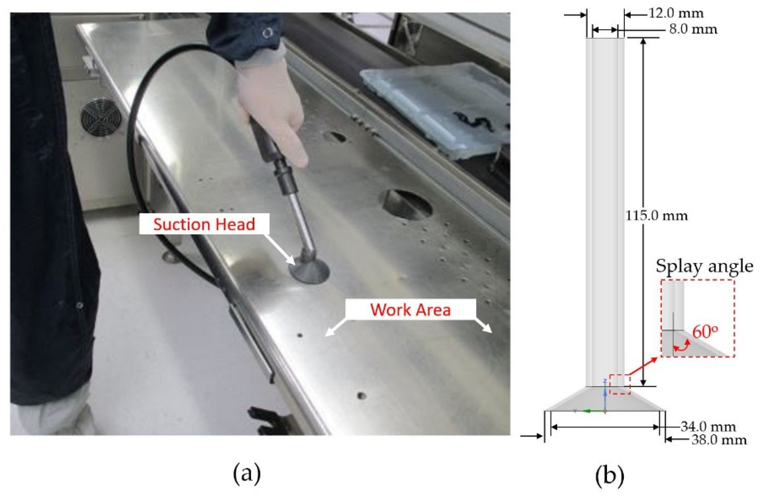
The actual SH of the factory was a bowl type with a handle that could be adjusted direction for convenience in operation and had a splay angle of 30° as shown in Figure 2a. Therefore, this research proposed new models with angles of 15°, 45°, 60°, 75°, and 90°, including the previous models with 0° and 30° in [12] as candidates for the suitable SH shape. Figure 2b shows an example of a splay angle of 60° as a fluid model created for simulation. In addition, the SH and duct were simplified to be connected without joints. A simplified model such as this helps avoid backflow. The backflow causes the calculation results to be incorrect and to diverge. The other SH shapes were precisely the same as in Figure 2b but differed only in the splay angles.
3.2. Simulation
3.2.1. Mesh Models
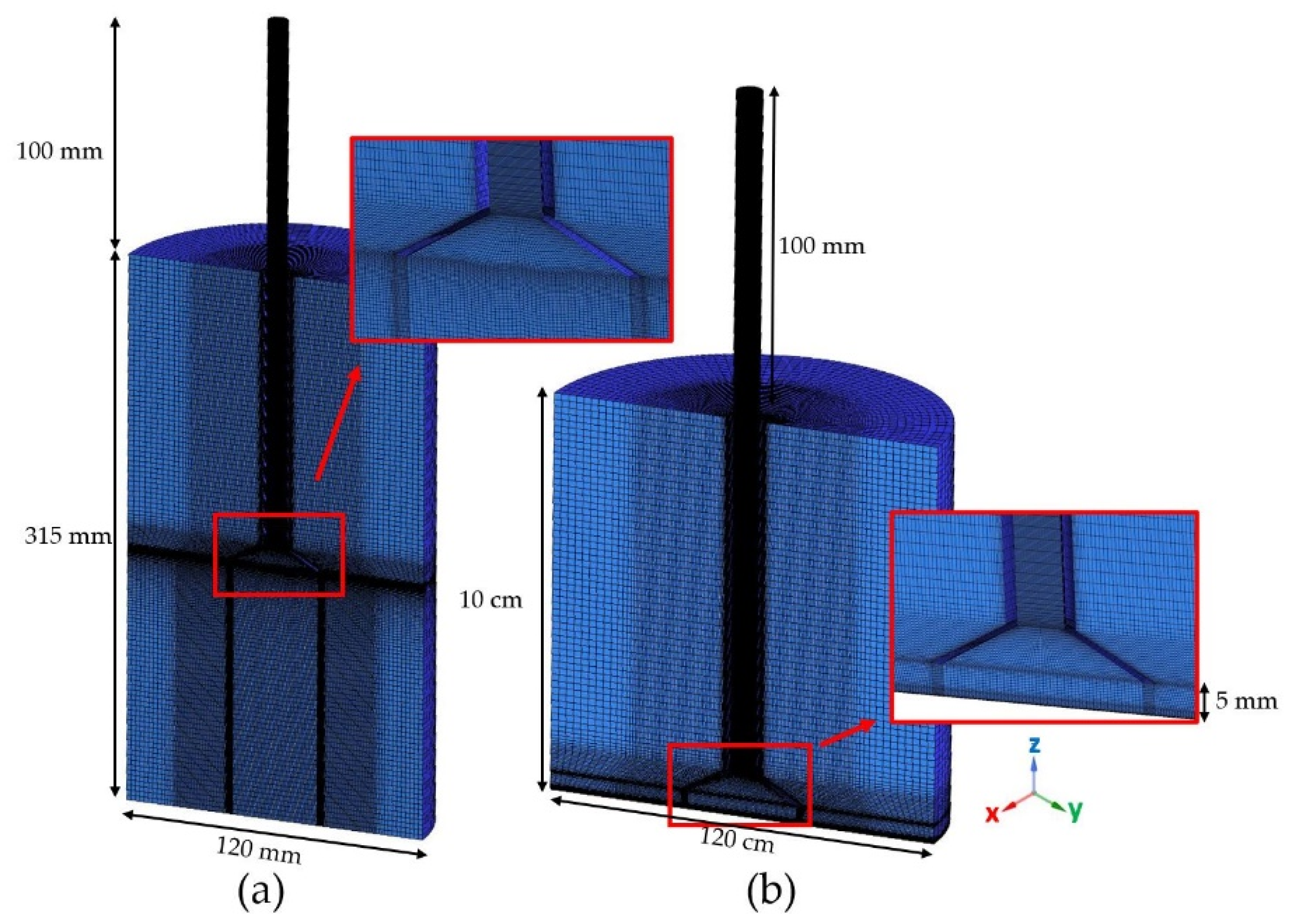
The fluid models mentioned above were used as prototypes to create mesh models using ICEM software specifically for creating a high-quality mesh model. Figure 3 shows the mesh models used to investigate the airflow (a) in space and (b) 5 mm above the work area. Both models were constructed as half models with all hexahedrons. The difference was that (a) had more space below the SH than (b). Both models were assigned y+ of 1 and a growth rate of 1.2, and then the ICEM software generated the mesh models automatically. The proper mesh models that provide reliable results with the fastest computational time based on mesh independent analysis have 0.86–0.92 million nodes and 0.89–0.93 million elements as shown in Figure 3a, and 0.43–0.47 million nodes and 0.40–0.44 million elements as shown in Figure 3b. Therefore, the proper mesh models have a minimum length of 0.1 mm and a maximum of 10 mm. We recognized that the estimated velocity of the fastest particles was 5 m/s [12], and the desired time step size was 1 × 10⁻³ s for the SST k-ω, so the element length recommended by the DPM should be higher than the multiplication between the velocity and time step size [20] which was 5 mm. Thus, the setting of element size as 0.1 mm in this research covered the recommendation of DP model. According to the mentioned recommendation, the elements of space around and below the SH in Figure 3b were smaller than the other regions to accurately capture the airflow and particle traces.
3.2.2. Boundary Conditions
The boundary conditions were reported only in the essential settings. For others not mentioned here, we used the default setting of the software. For example, Figure 4 shows the boundary conditions resulting from Figure 3. From the field measurement at the factory, we found that the splay angle of 30° pressure outside the SH was 101,375 Pa, while the pressure inside the pipe was 91,375 Pa, a difference of 10,000 Pa. Therefore, both pressures were defined as the pressure inlet and pressure outlet, respectively. The symmetry was the area where the airflows were precisely the same, which helps to generate a faster calculation. The air was set to 1255 kg/m3, an incompressible flow. The noise was generated when the air flowed through and impacted the SH’s surface; therefore, the SH was defined as a wall, representing a noise generated by the source in the FW–H model.
3.2.3. Software Settings
To investigate the particle removing performance, we used a one-way simulation with spherical particles of stainless steel of radius 0.5 μm and a density of 7500 kg/3 representing the dirt particles in the factory. In the one-way simulation, the airflow was calculated using Equations (1)–(4), and then the results were transferred to the particle trace calculation. The initial positions of 50,000 particles before removal were placed in a circle area with a radius of 6 cm and were written as a code in the Python programming language. Solving Equations (10) and (11) yielded particle traces and allowed the counting of particles before and after removal during 3 s. The mentioned method of setting was the same method that was successful in our previous work [6,12].
3.3. Experiment
Figure 5a shows the CAD models of SHs for various splay angles. Figure 5b shows actual SHs created by 3D printing using the CAD models above as prototypes. The inner surface of all the SHs was coated with wax to make it smooth, similar to the actual surface. The created SHs were employed to measure the air velocity and SPL in the experiment.
Figure 6a shows the installation of the equipment for air velocity measurement: an actual setup on the left and a schematic diagram on the right. First, the SH was installed at the end of a duct connected to a vacuum pump located far away to assure that the noise generated by the vacuum pump did not interfere with the experiment. Next, the vacuum pump was adjusted and monitored by a pressure gauge until the SH’s outside and inside pressures corresponded to the boundary conditions mentioned in Section 3.2.2. Finally, a Testo 425 hot-wire anemometer with ±0.03 m/s of accuracy was placed at a distance of 5 mm below the center of SH to measure the air velocity in space. The measurement was repeated five times.
Figure 6b reveals the implementation of the equipment for SPL measurement: an actual setup on the left and a schematic diagram on the right. Similar to the above, the hot-wire anemometer was replaced by a mobile phone with Decibel X v6.3.6. Decibel X is an application that received the highest rating in 2020. It can be used to measure the LAeq in the range of 40–85 dB very well, with discrepancies in the range of 0.9–2.3 dB [29]. The LAeq of frequencies in the range of 1000–4000 Hz were measured because this range is close to human listening. The microphone used was a Dayton Audio iMM-6, which was suitable for this experiment as it only provided an error of ±2 dB [30]. In addition, the microphone was encased in a windshield to prevent other noise sources from the environment. Before the experiment, the Decibel X was calibrated with a precise sound level meter to assure credible outcomes. The Decibel X recorded the frequency and SPL every 0.2 s, a total of 5 s to display the represented LAeq; again, the experiment was repeated five times. In fact, we had a basic but precise sound pressure meter, but it could measure only LAeq. Unfortunately, it could not report the A-weighted level frequency and had a large microphone compared to the diameter of SH, making it easier to affect the environment. Therefore, the Decibel X, Dayton, and the supported instruments were applied, as shown in Figure 6b. The decibel X required a post-processing procedure for analysis.
4. Results and Discussion
This section is divided into two subsections: validation and a suitable SH. First, the simulation and experimental results are reported to confirm the credibility of the research methodology. Later, all the results are analyzed along with the changes to some parameters that were introduced to find the suitable SH.
4.1. Validation
Figure 7 compares the air velocities from the simulation and the experiment for the suction in space displayed in Figure 6a. The comparison shows good consistency, with the simulation error in the range of 1.52–3.95% compared to the average value. The SH’s shapes affected the air velocity at the measured point. The simulation results reveal that 90° SH gave the highest air velocity of 5.78 m/s, while 45° SH gave the lowest value of 3.52 m/s. The error may be that the wind speed flowing out of the SH was unstable and changed slightly, but we used the constant pressure in the boundary condition. Hence, using the transient pressure profile setting as the boundary condition will decrease the error as suggested in [6]. Moreover, increasing the number of measurements is expected to reduce the error. The error bars represented the standard deviation from the experiment were in the range of 0.13–0.23 m/s, higher than the uncertainty (resolution) of hot-wire anemometer of ±0.03 m/s (Testo 425). However, all the simulation results were still within the error bar of height, so the simulation results of air velocity are reliable.
With the same boundary condition as above, Table 3 shows the simulation (Sim.) and experimental (Exp.) results from the experiment displayed in Figure 6b for 1/3 octave band frequencies in the 1000–4000 Hz range of 15°, 45°, and 90° SHs. In the first column, 890.9–1125.5 Hz, 1122.6–1414.2 Hz, and so on are the frequency ranges of the theoretical A-weighted SPL. The standard frequencies reported by Decibel X are in parentheses. The second column shows the simulation frequencies calculated by the LES and FW–H models in CFD. The parentheses report a discrepancy relative to the standard frequency, which ranges from 0.3 to 1%. Thus, again, the simulation frequencies were still within the theoretical frequency range and are reliable. We use the word “discrepancy” because both the simulation and experiment results had their own errors. Therefore, it is impossible to determine which one is the most accurate, unlike the anemometer measurement, which we believe provides highly accurate results compared to the simulation. In columns 3–8, the LAeq of simulation and measurement are reported. All the experimental results were less than all of the simulations; we expected this because of the windshield. Without the windshield, we found that the LAeq was unstable due to the noise generated by the environment, so we preferred to install the windshield. The bottom row reports the total LAeq from the experiment measured by Decibel X and the simulation calculated using Equation (16) and the data above in the same column. The LAeq in the asterisk reported by Decibel X included the sound pressure level from other frequencies outside Table 3. Their values are close to those obtained in simulation, implying that noise due to other frequencies had little effect on the SPL since 1000–4000 Hz is the range frequency of human listening, as expected. Based on the results in Table 3, we believe that the simulation results of LAeq are also credible.
Increasing the credibility and reducing the simulation discrepancy can be achieved by improving the number of time steps and the time step size to cover a longer time. In addition, enhancing the accuracy and minimizing the experimental errors can be approached using a high-precision anemometer and sound pressure level instruments to improve the measurement with more repetitions. However, we believe that such improvements will not affect our conclusions since the simulation and experiment described above have already yielded reliable and sufficient results. Therefore, the research methodology could be applied to determine the suitable SH shape in the next subsection.
4.2. A Suitable SH Shape
This section has been divided into two parts: suction performance and noise generation. The results from two parts were analyzed to find a suitable SH.
4.2.1. Suction Performance
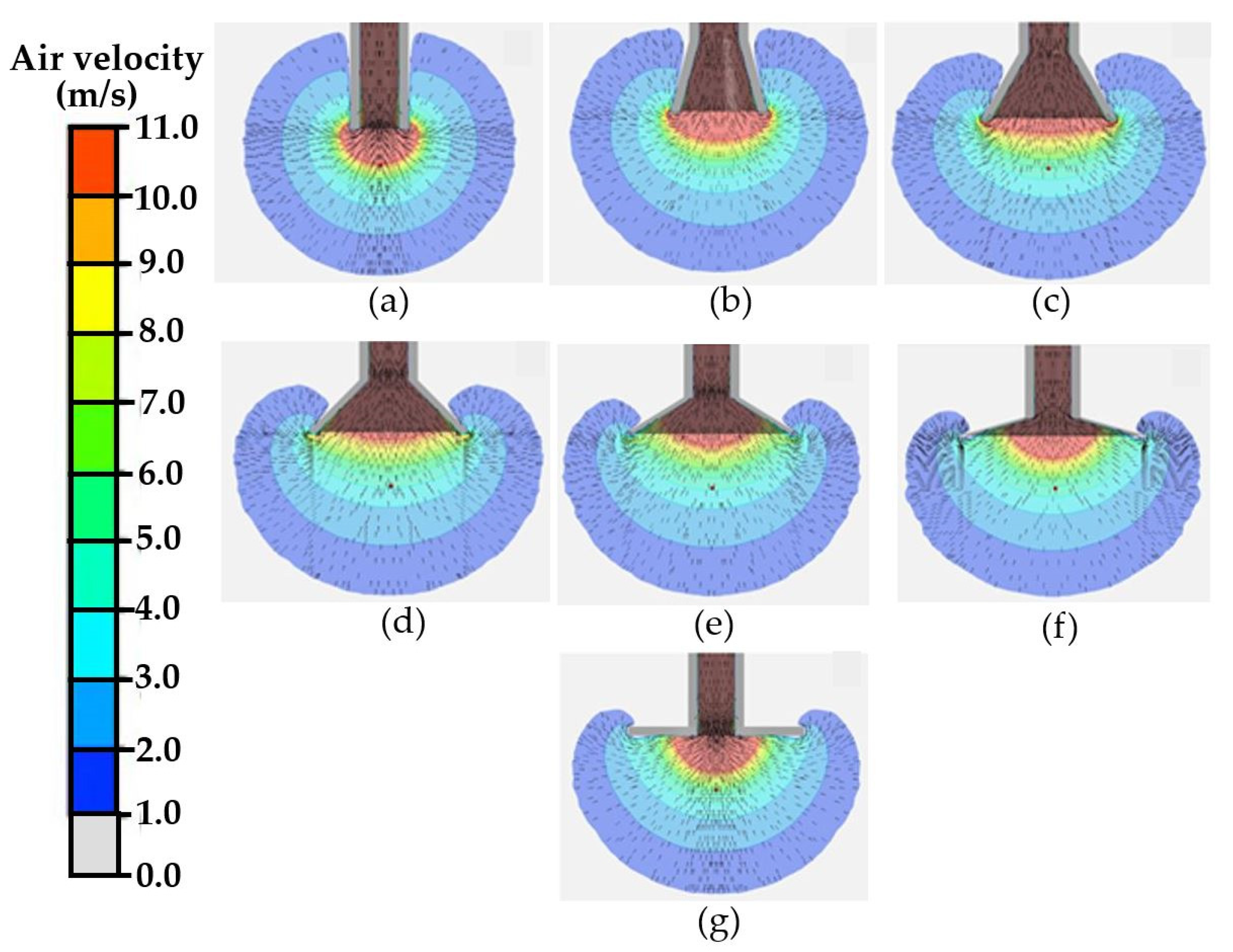
As described in Section 3.2.2 and Section 3.2.3, the stainless-steel particles represented the dirt particles to be cleaned in the factory. Therefore, solving Equation (5), the suspension velocity (vs) was 1.0114 m/s. Figure 8 shows the contour plots of the cleaning region in 2D in a center plane simulated by the SST k-ω, that is, the region with air velocity perpendicular to the work area higher than vs for the splay angles of (a) 0°, (b) 15°, (c) 30°, (d) 45°, (e) 60°, (f) 75°, and (g) 90°. The grey color is the unclean region; the dirt particles cannot be removed. The small vectors in the black color confirmed that the air was sucked into the SH. The red color is the region with an air velocity higher than 10 m/s. The simulation results reveal that different SH shapes gave different cleaning region shapes; they had unequal performances. For (a)–(g), the cleaning regions in space were (a) 354.96 mm2, (b) 420 mm2, (c) 436.64 mm2, (d) 474.80 mm2, (e) 477.09 mm2, (f) 476.48 mm2, and 481.82 mm2. Similarly, Figure 9 shows the cleaning regions for the pressures of 10,000 Pa, 50,000 Pa, and 100,000 Pa. Note that 10,000 Pa is the difference between the pressure inlet and pressure outlet. When increasing the pressure difference or enhancing the vacuum pump’s level, the cleaning region would be enlarged; particles could be removed in a larger area, as expected. The higher the pressure, the better the cleaning performance. From Figure 8 and Figure 9, the 0° SH provided the smallest cleaning region consistent with the report in [12], while 45°, 60°, 75°, and 90° SHs provided similar cleaning region sizes and were larger than the others. Therefore, they were the shapes that were potential suitable models that needed to be investigated further. The SHs with small splay angles are less efficient because they also suck the air on the top, which is not the target area in the cleaning process. Powerful SHs are often designed to have just the proper splay angle [12,13,14,15,16,17,18].
Figure 10a–g reveal the cleaning regions in a side view of the work area with a different pressure of 10,000 Pa for the 0°–90° SHs, respectively. Similarly, Figure 11a–g show the view of the cleaning regions from the top, displayed using the vs perpendicular to the work area. The circle area with a radius of 6 cm is a target region expected to be cleaned. The cleaning region is the area represented by color. On the contrary, the grey color is where particles are not sucked into the SH, and no cleaning occurs. To the naked eye, it is impossible to determine the sizes of the cleaning regions in Figure 11, so a computer needs to be employed to help analyze the data. This is discussed together with the results of particle trace next.
Figure 12 shows the samples of the remaining stainless steel particle traces after 3 s of cleaning, simulated using the SST k-ω and DPM models for (a) 0°, (b) 30°, and (c) 45°. Again, the color scale reports the particle velocity, and the streak presents its trace. The closer the position to the SH, the higher the removal particle velocity, as expected. With careful observation, it can be seen that the 45° SH had the fewest particles remaining in the work area; that is, it removed the most particles, followed by the 30° SH, and finally, the 0° SH was the worst at removing the particles. In fact, we simulated the cleaning process of all the SHs, but we have shown only three samples because the resulting images were very similar. Displaying all the SHs does not aid analysis and may be confusing because the remaining particles cannot be counted visually. Therefore, a computer was used to help us accurately count the number of remaining and sucked-up particles. Again, we will discuss them next.
Figure 13 shows the cleaning regions from Figure 11 and the particle removing performance from Figure 12 for various SH shapes. The particle removing performance is the percentage of particles present in the work area calculated before and after cleaning. Again, the comparison revealed consistency. The SH shapes affected the cleaning region and the particle removing performance. As expected, the 30° SH was better than the 0° SH, consistent with the report in [12], but it was not the best. The 75° SH was the model with the best particle removing performance of 84.66% with a cleaning region of 270 mm2.
4.2.2. Noise Generation
Figure 14 shows the LAeq and frequencies simulated with the LES and FW–H models for various SH shapes. All simulation results confirm that the SH shapes affected the LAeq. For all frequencies, the 90° SH generated the highest noise, 45° SH generated the lowest. Comparing Figure 7 and Figure 8, the noise was related to the air velocity. The higher the air velocity, the higher the noise generation, as expected. The relationship is confirmed by Equations (12)–(14) in the FW–H model, which shows that air velocity (u) is a significant factor of noise generation. In summary, Table 4 reports the results from Figure 13 and Figure 14.
Although the 75° SH had the largest cleaning region and the best particle removing performance, it generated high amounts of noise. On the other hand, the 45° SH had the lowest noise but moderated the cleaning region of 190 mm2. It had a removing performance of 79.23%, and the lowest total LAeq of 32.2 dB. In our opinion, it stands out from the other shapes because it had a particle removing performance of 5.43% and a total LAeq of 28.4 less than the 75° SH. Therefore, it is well balanced in terms of particle removing performance and noise generation. Additionally, the 45° SH had 40 mm2 more cleaning region, a 4.37% higher particle removing performance, and produced 11.1 dB less total LAeq than the 30° SH currently used in the problematic factory. Therefore, from the results reported in Figure 7, Figure 8, Figure 9, Figure 10, Figure 11, Figure 12, Figure 13 and Figure 14, we concluded that the 45° SH is a suitable shape for the cleaning process of the factory. The finding of this research has been forwarded to the factory. As a result, it was accepted and implemented in the actual cleaning process.
5. Conclusions
To improve the cleaning process in a factory, we proposed new shapes of SH with splay angles of 15°, 45°, 60°, 75°, and 90°, including 0° and 30° from previous work. A total of seven models were used to investigate the particle removing performance and sound noise generation using CFD in a transient state. The investigation was divided into two usage situations: in space and 5 mm above the work area. First, the SST k-ω turbulence and DP models were employed to determine the air velocity, cleaning region, suspension velocity, and particle trace. Then, the LES and FW–H models were used to calculate SPL and frequency generated by various shapes of SH. Next, the simulated air velocity was validated by a hot-wire anemometer, while the simulated SPL and frequency were confirmed by a Decibel X, an application in a mobile phone, so the simulation results were credible. Then, all the results were analyzed in both usage situations and showed that the shape of SH affected the cleaning region, particle removing performance, and noise generation, as expected. The 90° SH generated the highest amount of annoying noise, but the 45° SH created the lowest. The 75° SH gave the largest cleaning region; however, the 0° SH provided the smallest. The 75° SH had the highest particle removing performance, yet the 0° SH had the worst. The more pressure used for cleaning, the larger the cleaning region and the greater the particle removing performance. The higher the air velocity released by the SH, the greater the noise generation. Finally, all results were analyzed. We concluded that the 45° SH was the most suitable shape for the cleaning process because it stood out in particle removing performance and noise generation, and was better than the previous shape.
Author Contributions
Conceptualization, J.T. and J.K.; methodology, J.T. and J.K.; software, J.T., W.T. and J.K.; validation, J.T. and J.K., formal analysis, J.T.; investigation, J.T.; writing—original draft preparation, J.T.; writing—review and editing, J.T.; project administration, J.T.; funding acquisition, J.T. All authors have read and agreed to the published version of the manuscript.
Funding
The fund was sponsored by Research and Researchers for Industry (RRI), a grant number MSD60I0126.
Institutional Review Board Statement
Not applicable.
Informed Consent Statement
Not applicable.
Data Availability Statement
No additional data available.
Acknowledgments
This research was supported by the College of Advanced Manufacturing Innovation, King Mongkut’s Institute of Technology Ladkrabang, and Seagate Technology (Thailand) Ltd.
Conflicts of Interest
The authors declare that there are no conflict of interest for this article.
References
- ISO. Cleanrooms and Associated Controlled Environment—Part 1: Classification of Air Cleanliness; ISO No. 146441-1; ISO: Geneva, Switzerland, 1999. [Google Scholar]
- Thongsri, J. A Successful CFD-Based Solution to a Water Condensation Problem in a Hard Disk Drive Factory. IEEE Access 2017, 5, 10795–10804. [Google Scholar] [CrossRef]
- Sandle, T. Distribution of Particles within the Cleanroom: A Review of Contamination Control Considerations. J. GXP Compliance 2017, 21, 1–10. [Google Scholar]
- Naosungnoen, J.; Thongsri, J. Airflow and Temperature Simulation in a Big Cleanroom to Reduce Contamination in an HDD Manufacturing Factory. IOP Conf. Ser. Mater. Sci. Eng. 2018, 361, 012025. [Google Scholar] [CrossRef]
- Romano, F.; Milani, S.; Joppolo, C.M. Airborne Particle and Microbiological Human Emission Rate Investigation for Cleanroom Clothing Combinations. Build. Environ. 2020, 180, 106967. [Google Scholar] [CrossRef]
- Thongsri, J. A Problem of Particulate Contamination in an Automated Assembly Machine Successfully Solved by CFD and Simple Experiments. Math. Probl. Eng. 2017, 2017, 6859852. [Google Scholar] [CrossRef] [Green Version]
- Khaokom, A.; Thongsri, J.; Kaewkhaw, P. A CFD Investigation of Airflow in a Hard Disk Drive Production Line to Detect The Cause(s) of Contamination and Its Mitigation. In Proceedings of the 2017 IEEE 3rd International Conference on Engineering Technologies and Social Sciences (ICETSS), Bangkok, Thailand, 7–8 August 2017; pp. 1–4. [Google Scholar]
- Puangburee, L.; Busayaporn, W.; Kaewbumrung, M.; Thongsri, J. Evaluation and Improvement of Ventilation System Inside Low-Cost Automation Line to Reduce Particle Contamination. ECTI Trans. Electr. Eng. Electron. Commun. 2020, 18, 35–44. [Google Scholar] [CrossRef] [Green Version]
- Zhivov, A.; Skistad, H.; Mundt, E.; Posokhin, V.; Ratcliff, M.; Shilkrot, E.; Strongin, A.; Li, X.; Zhang, T.; Zhao, F.; et al. Chapter 7—Principles of Air and Contaminant Movement Inside and Around Buildings. In Industrial Ventilation Design Guidebook, 2nd ed.; Goodfellow, H.D., Kosonen, R., Eds.; Academic Press: Cambridge, MA, USA, 2020; pp. 245–370. [Google Scholar]
- Jai-Ngam, N.; Tangchaichit, K. Simulation of Airflow inside a Computer Hard Disk Drive to Develop an Impinging Air Jet Particle Detachment System for Cleaning Head Stack Assemblies. IEEE Trans. Magn. 2018, 54, 1–8. [Google Scholar] [CrossRef]
- Yimsiriwatana, N.; Jearsiripongkul, T. Airflow Simulation of Particle Suction in Hard Disk Drives Manufacturing Process. Int. Rev. Model. Simul. 2011, 4, 429–435. [Google Scholar]
- Khongsin, J.; Thongsri, J. Numerical Investigation on the Performance of Suction Head in a Cleaning Process of Hard Disk Drive Factory. ECTI Trans. Electr. Eng. Electron. Commun. 2020, 18, 28–34. [Google Scholar] [CrossRef] [Green Version]
- Dalla, V.J.M. Exhaust Hoods; Industrial Press: New York, NY, USA, 1952. [Google Scholar]
- Garrison, R.P. Nozzle Performance and Design for High Velocity/Low Volume Exhaust Ventilation; ProQuest Information & Learning: Ann Arbor, MI, USA, 1977. [Google Scholar]
- Fletcher, B. Centreline Velocity Characteristics of Rectangular Unflanged Hoods and Slots Under Suction*©. Ann. Occup. Hyg. 1977, 20, 141–146. [Google Scholar] [CrossRef] [PubMed]
- Tyaglo, I.G.; Shepelev, I.A. Air Flow Near Exhaust Opening. Vodosnabzheniye i Sanitarnaya Tekhnika 1970, 5, 24–25. [Google Scholar]
- Posokhin, V.N.; Zhivov, A.M. Principles of Local Exhaust Design. In Proceedings of the 5th International Symposium on Ventilation for Contaminant Control, Ottawa, ON, Canada, 14–17 September 2021; Canadian Environment Industry Association: Ottawa, ON, Canada, 1997; Volume 1. [Google Scholar]
- He, X.; Lewis, B.V.; Guffey, S.E. Experimental Study on Centerline Velocities of a Rectangular Capture Hood Under Realistic Conditions. J. Occup. Environ. Hyg. 2018, 15, 125–132. [Google Scholar] [CrossRef] [PubMed]
- Zhang, J.; Wang, J.; Gao, J.; Xie, M.; Cao, C.; Lv, L.; Zeng, L. Experimental and Numerical Study of The Effect of Perimeter Jet Enhancement on The Capture Velocity of a Rectangular Exhaust Hood. J. Build. Eng. 2020, 33, 101652. [Google Scholar] [CrossRef]
- Ansys Inc. Chapter 16 Discrete phase. In Ansys Fluent 17.1, User’s Guide; Ansys Inc.: Canonsburg, PA, USA, 2016. [Google Scholar]
- Cianferra, M.; Ianniello, S.; Armenio, V. Assessment of Methodologies for The Solution of The Ffowcs Williams and Hawkings Equation Using LES of Incompressible Single-phase Flow Around a Finite-size Square Cylinder. J. Sound Vib. 2019, 453, 1–24. [Google Scholar] [CrossRef]
- Lallier-Daniels, D.; Piellard, M.; Coutty, B.; Moreau, S. Aeroacoustic Study of an Axial Engine Cooling Module Using Lattice-Boltzmann Simulations and The Ffowcs Williams and Hawkings’ Analogy. Eur. J. Mech. B/Fluids 2017, 61, 244–254. [Google Scholar] [CrossRef]
- Zhiyin, Y. Large-Eddy Simulation: Past, present and the future. Chin. J. Aeronaut. 2015, 28, 11–24. [Google Scholar] [CrossRef] [Green Version]
- Ansys Inc. Chapter 15 Aerodynamically Generated Noise. In Ansys Fluent 17.1, User’s Guide; Ansys Inc.: Canonsburg, PA, USA, 2016. [Google Scholar]
- Ansys Inc. Chapter 4 Turbulence. In Ansys Fluent 17.1, User’s Guide; Ansys Inc.: Canonsburg, PA, USA, 2016. [Google Scholar]
- Ansys Inc. Chapter 18 Multiphase Flows. In Ansys Fluent 17.1, User’s Guide; Ansys Inc.: Canonsburg, PA, USA, 2016. [Google Scholar]
- Jansaengsuk, T.; Kaewbumrung, M.; Busayaporn, W.; Thongsri, J. A Proper Shape of the Trailing Edge Modification to Solve a Housing Damage Problem in a Gas Turbine Power Plant. Processes 2021, 9, 705. [Google Scholar] [CrossRef]
- Castle Group. What Is Leq and How Is It Measured. Available online: https://www.castlegroup.co.uk/what-is-leq/ (accessed on 2 September 2021).
- Brown, P.; Biggs, T.; Crossley, E.; Singh, T. The Accuracy of iPhone Applications to Monitor Environmental Noise Levels. Laryngoscope 2020, 131. [Google Scholar] [CrossRef]
- Kardous, C.A.; Shaw, P.B. Evaluation of Smartphone Sound Measurement Applications (apps) Using External Microphones—A Follow-up Study. J. Acoust. Soc. Am. 2016, 140, EL327–EL333. [Google Scholar] [CrossRef] [Green Version]
Figure 1.
A flowchart of the research methodology.

Figure 2.
A suction head: (a) actual model in a factory [12], and (b) simplified fluid model in a simulation.
Figure 2.
A suction head: (a) actual model in a factory [12], and (b) simplified fluid model in a simulation.

Figure 3.
Mesh models for simulation in (a) space and (b) 5 mm above the work area.

Figure 4.
Boundary conditions for simulation in (a) space and (b) 5 mm above the work area.

Figure 5.
Suction heads (a) CAD model, and (b) actual models created by 3D printing.

Figure 6.
Actual experimental setups on the left and schematic diagrams on the right for (a) air velocity and (b) sound pressure level measurements.
Figure 6.
Actual experimental setups on the left and schematic diagrams on the right for (a) air velocity and (b) sound pressure level measurements.

Figure 7.
Comparison between the simulated and measured air velocities.

Figure 8.
Th cleaning regions for the splay angles of (a) 0°, (b) 15°, (c) 30°, (d) 45°, (e) 60°, (f) 75°, and (g) 90°.
Figure 8.
Th cleaning regions for the splay angles of (a) 0°, (b) 15°, (c) 30°, (d) 45°, (e) 60°, (f) 75°, and (g) 90°.

Figure 9.
The cleaning regions for the different pressures.

Figure 10.
The cleaning regions in a side view of the work area for the splay angles of (a) 0°, (b) 15°, (c) 30°, (d) 45°, (e) 60°, (f) 75°, and (g) 90°.
Figure 10.
The cleaning regions in a side view of the work area for the splay angles of (a) 0°, (b) 15°, (c) 30°, (d) 45°, (e) 60°, (f) 75°, and (g) 90°.

Figure 11.
The cleaning regions in a top view of the work area for the splay angles of (a) 0°, (b) 15°, (c) 30°, (d) 45°, (e) 60°, (f) 75°, and (g) 90°.
Figure 11.
The cleaning regions in a top view of the work area for the splay angles of (a) 0°, (b) 15°, (c) 30°, (d) 45°, (e) 60°, (f) 75°, and (g) 90°.

Figure 12.
The remaining particles after 3 s of the cleaning process of the splay angles of (a) 0°, (b) 30°, (c) 45° SHs.
Figure 12.
The remaining particles after 3 s of the cleaning process of the splay angles of (a) 0°, (b) 30°, (c) 45° SHs.

Figure 13.
The cleaning regions and percentage of removing particles for various SH shapes.

Figure 14.
The equivalent A-weighted SPLs (LAeq) and frequencies for various SH shapes.


Table 1.
The essential settings for the SST k-ω simulation.
| Solver | Pressure Based (Transient) |
|---|---|
| Turbulence model | SST k-ω |
| Solution method | Coupled (Second-order upwind) |
| Residual | 1 × 10⁻⁴ |
| Time step size | 1 × 10⁻³ s |
| Number of time steps (20 iteration/time steps) | 3000 steps |
Table 2.
The essential settings for the LES simulation.
| Solver | Pressure Based (Transient) |
|---|---|
| Turbulence model | Large Eddy Simulation (LES) |
| Solution method | Non-Iterative Time Advancement method |
| The pressure-velocity coupling method: Fractional Step | |
| Pressure spatial discretization: linear | |
| The gradient discretization: Least squares cell-based scheme | |
| The momentum: Bounded Central Differencing | |
| Transient Formulation: Second-Order Implicit | |
| Acoustic model | Ffowcs William and Hawkings (FW–H) |
| Acoustic source: source zone: nozzle wall | |
| Number of time steps per file = 1000 | |
| Residual | 1 × 10⁻⁴ |
| Time step size | 5 × 10⁻⁶ s |
| Number of time steps (10 iteration/time steps) | 10,000 steps |
Table 3.
Equivalent A-weighted sound pressure level at 5 mm below the center point of SH.
| 1/3 Octave Band Frequency (Hz) | LAeq (dBA) | ||||||
|---|---|---|---|---|---|---|---|
| 15° | 45° | 90° | |||||
| Exp. (Standard) | Sim. (Discrepancy%) | Exp. | Sim. | Exp. | Sim | Exp. | Sim. |
| 890.9–1125.5 (1000) | 1006 (0.6%) | 54.2 ± 5.1 | 55.6 | 32.2 ± 7.2 | 34.2 | 69.2 ± 5.5 | 72.5 |
| 1122.6–1414.2 (1250) | 1260 (0.8%) | 50.2 ± 4.7 | 54.5 | 32.4 ± 6.1 | 34.9 | 68.4 ± 5.2 | 71.7 |
| 1414.3–1781.8 (1600) | 1600 (0.0%) | 53.1 ± 4.8 | 54.2 | 30.2 ± 6.0 | 31.3 | 67.5 ± 5.7 | 71.8 |
| 1781.9–2244.9 (2000) | 2020 (1.0%) | 54.0 ± 5.2 | 56.1 | 29.8 ± 5.3 | 32.8 | 67.8 ± 5.3 | 70.3 |
| 2245.0–2828.4 (2500) | 2520 (0.8%) | 53.2 ± 4.8 | 56.9 | 27.9 ± 6.8 | 30.3 | 68.2 ± 5.4 | 71.6 |
| 2828.5–3563.6 (3150) | 3175 (0.8%) | 53.4 ± 5.0 | 57.3 | 27.5 ± 5.4 | 28.9 | 67.8 ± 5.3 | 72.9 |
| 3563.6–4489.8 (4000) | 4010 (0.3%) * | 50.3 ± 4.7 | 52.9 | 27.8 ± 6.7 | 28.6 | 70.3 ± 5.5 | 73.9 |
| Total LAeq | 53.6 ± 5.6 * | 55.6 | 30.8 ± 4.6 * | 32.2 | 69.2 ± 6.1 * | 72.2 | |
Table 4.
The performance of the SHs.
| Splay Angle | Cleaning Performance | Total LAeq (dB) | |
|---|---|---|---|
| Cleaning Region (mm2) | Particle Removing Performance (%) | ||
| 0° | 60 | 52.37 | 68.3 |
| 15° | 100 | 63.79 | 55.6 |
| 30° | 150 | 74.86 | 43.3 |
| 45° | 190 | 79.23 | 32.2 |
| 60° | 220 | 82.61 | 46.8 |
| 75° | 270 | 84.66 | 60.6 |
| 90° | 90 | 57.74 | 72.2 |
Publisher’s Note: MDPI stays neutral with regard to jurisdictional claims in published maps and institutional affiliations. |
© 2021 by the authors. Licensee MDPI, Basel, Switzerland. This article is an open access article distributed under the terms and conditions of the Creative Commons Attribution (CC BY) license (https://creativecommons.org/licenses/by/4.0/).
Share and Cite
MDPI and ACS Style
Thongsri, J.; Tangsopa, W.; Khongsin, J. A Suitable Shape of the Suction Head for a Cleaning Process in a Factory Developed by Computational Fluid Dynamics. Processes 2021, 9, 1902. https://0-doi-org.brum.beds.ac.uk/10.3390/pr9111902
AMA Style
Thongsri J, Tangsopa W, Khongsin J. A Suitable Shape of the Suction Head for a Cleaning Process in a Factory Developed by Computational Fluid Dynamics. Processes. 2021; 9(11):1902. https://0-doi-org.brum.beds.ac.uk/10.3390/pr9111902
Chicago/Turabian StyleThongsri, Jatuporn, Worapol Tangsopa, and Jirawat Khongsin. 2021. "A Suitable Shape of the Suction Head for a Cleaning Process in a Factory Developed by Computational Fluid Dynamics" Processes 9, no. 11: 1902. https://0-doi-org.brum.beds.ac.uk/10.3390/pr9111902
Note that from the first issue of 2016, this journal uses article numbers instead of page numbers. See further details here.