
Numerical Study on the Aerodynamic Characteristics of the NACA 0018 Airfoil at Low Reynolds Number for Darrieus Wind Turbines Using the Transition SST Model


Abstract
:1. Introduction
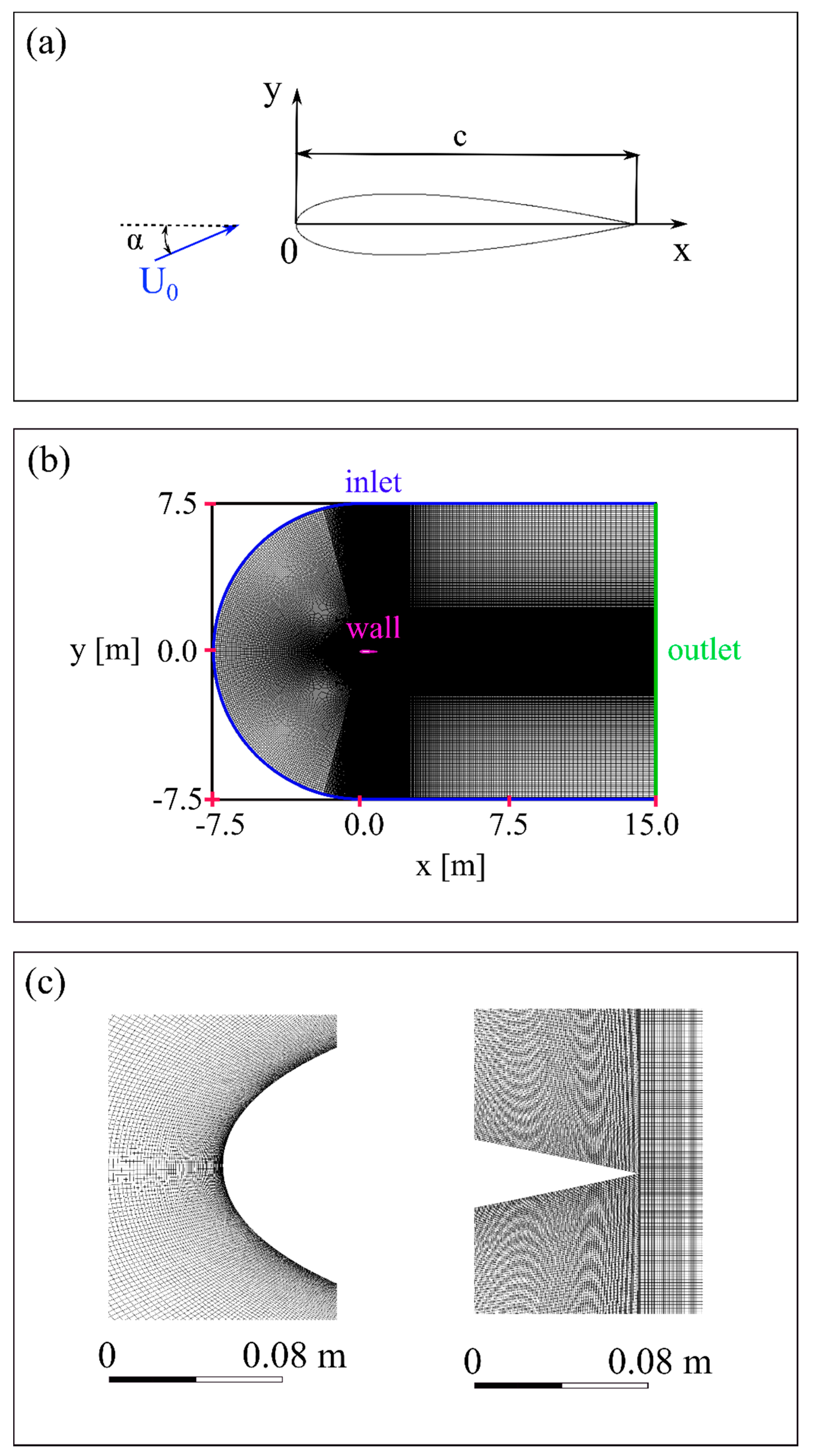
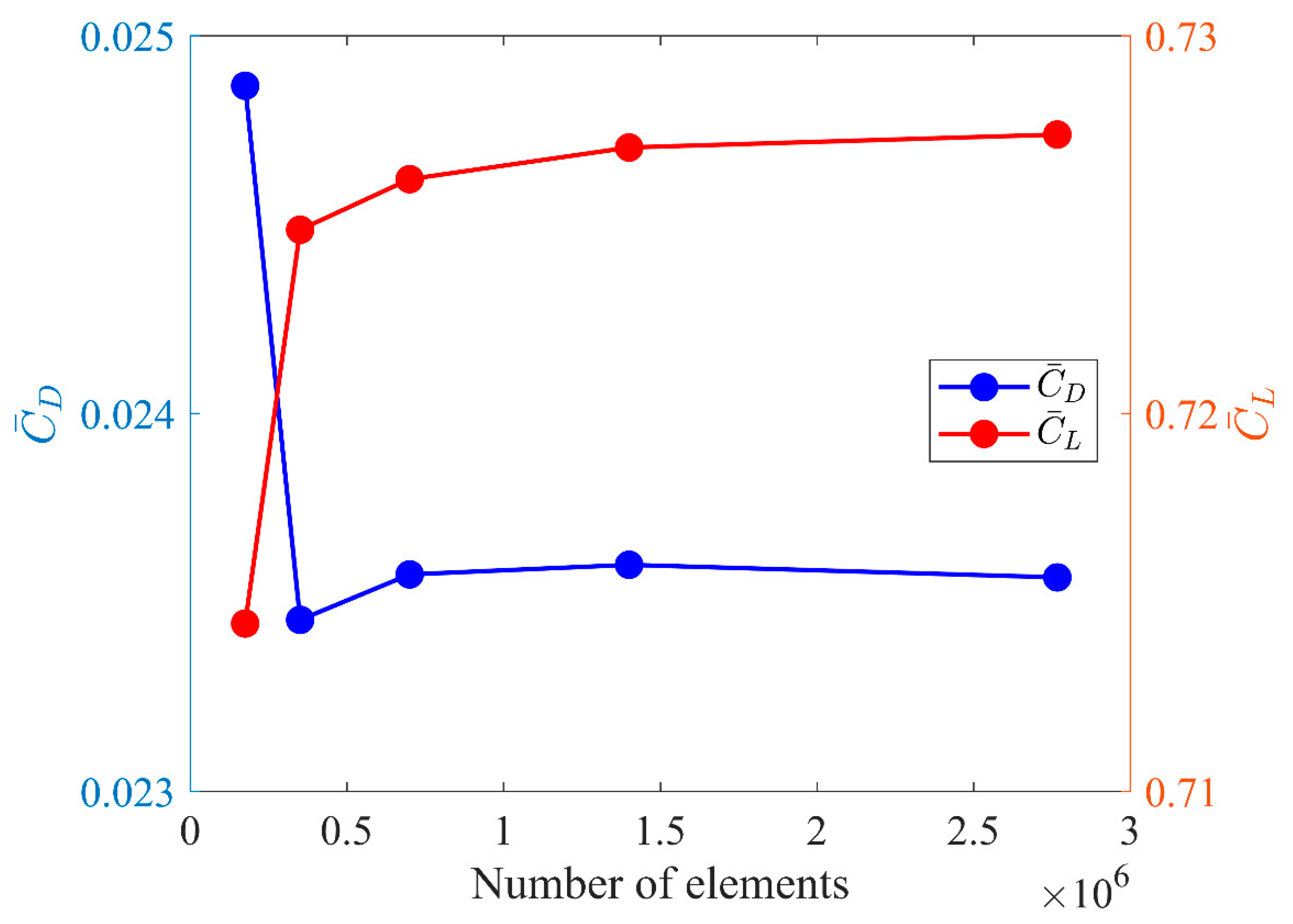
2. Numerical Methods
3. Simulation Results and Validation
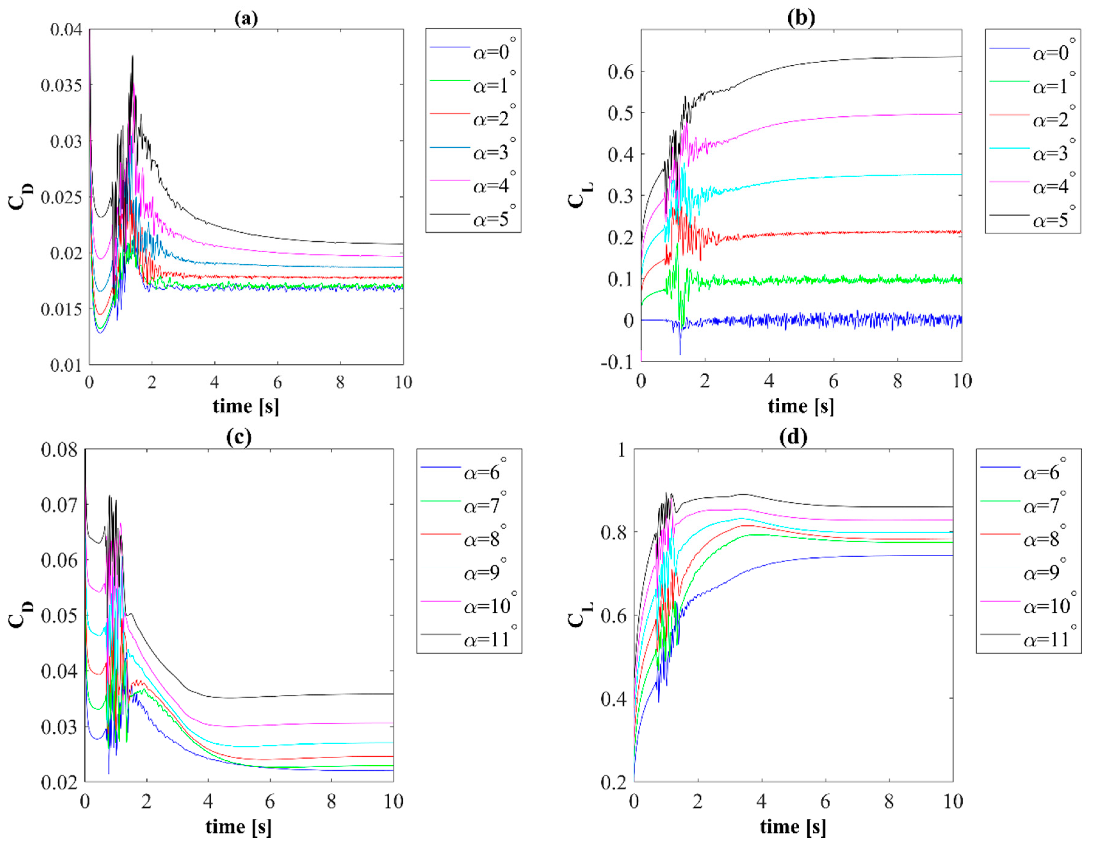
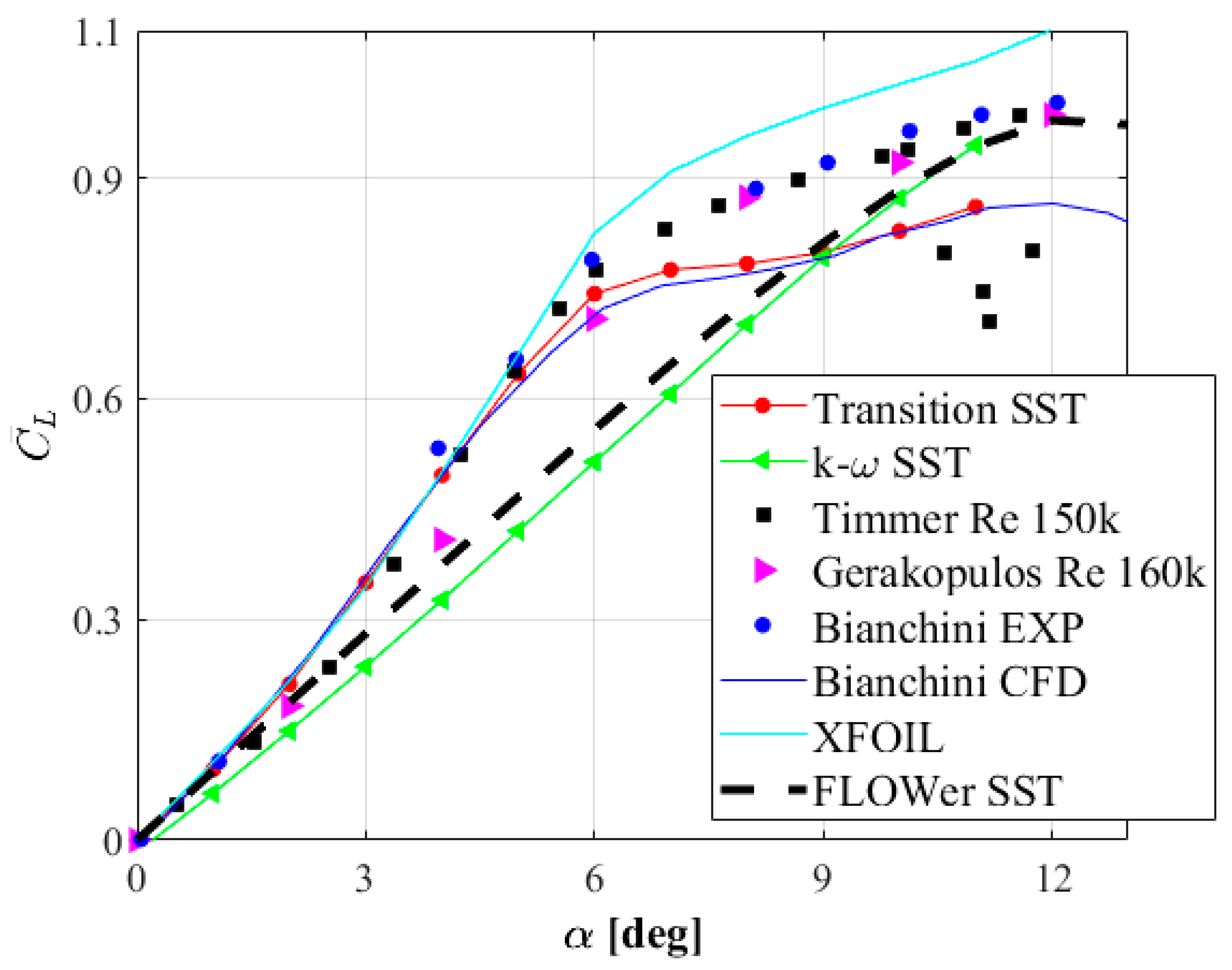
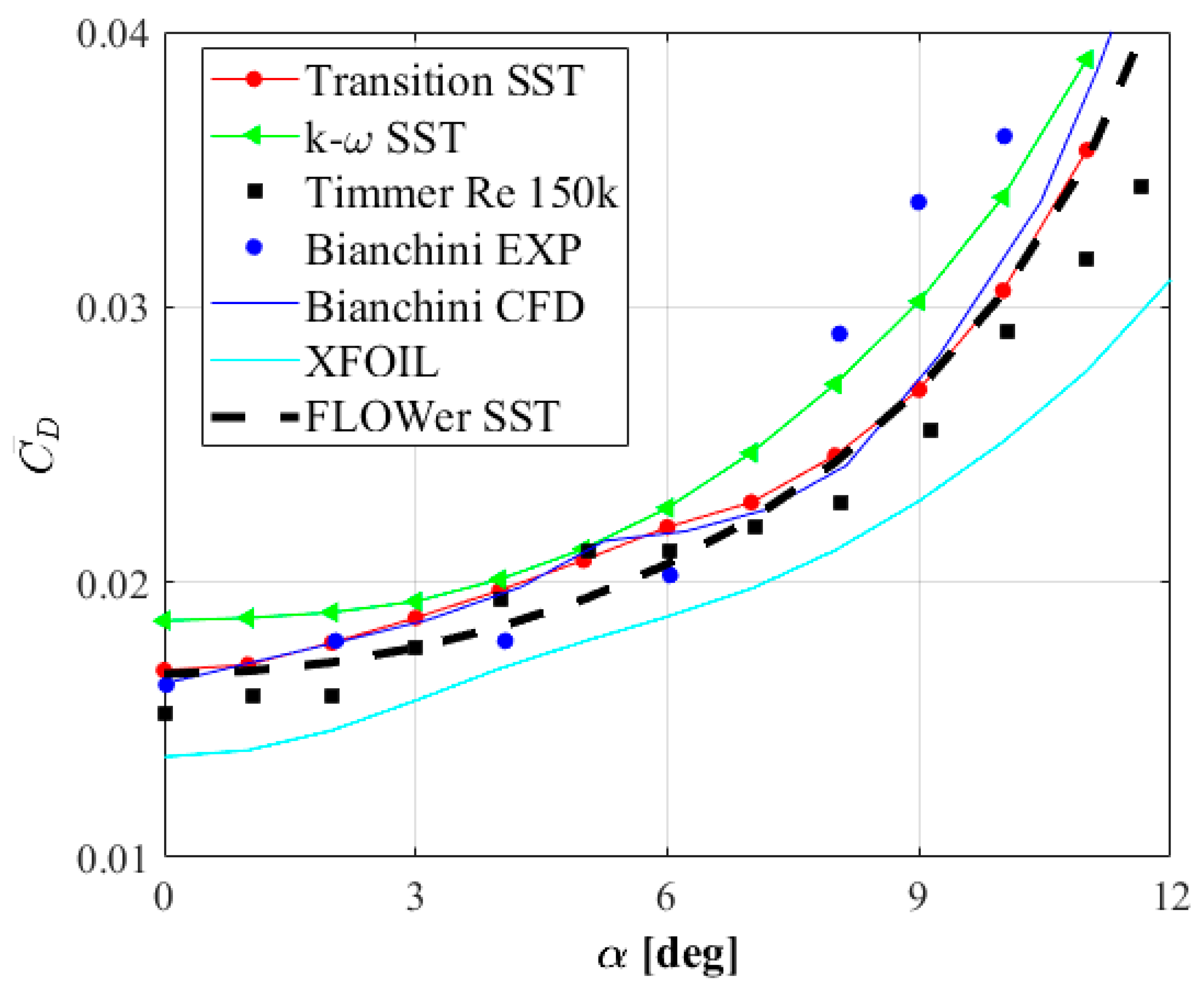
3.1. Lift and Drag Coefficients
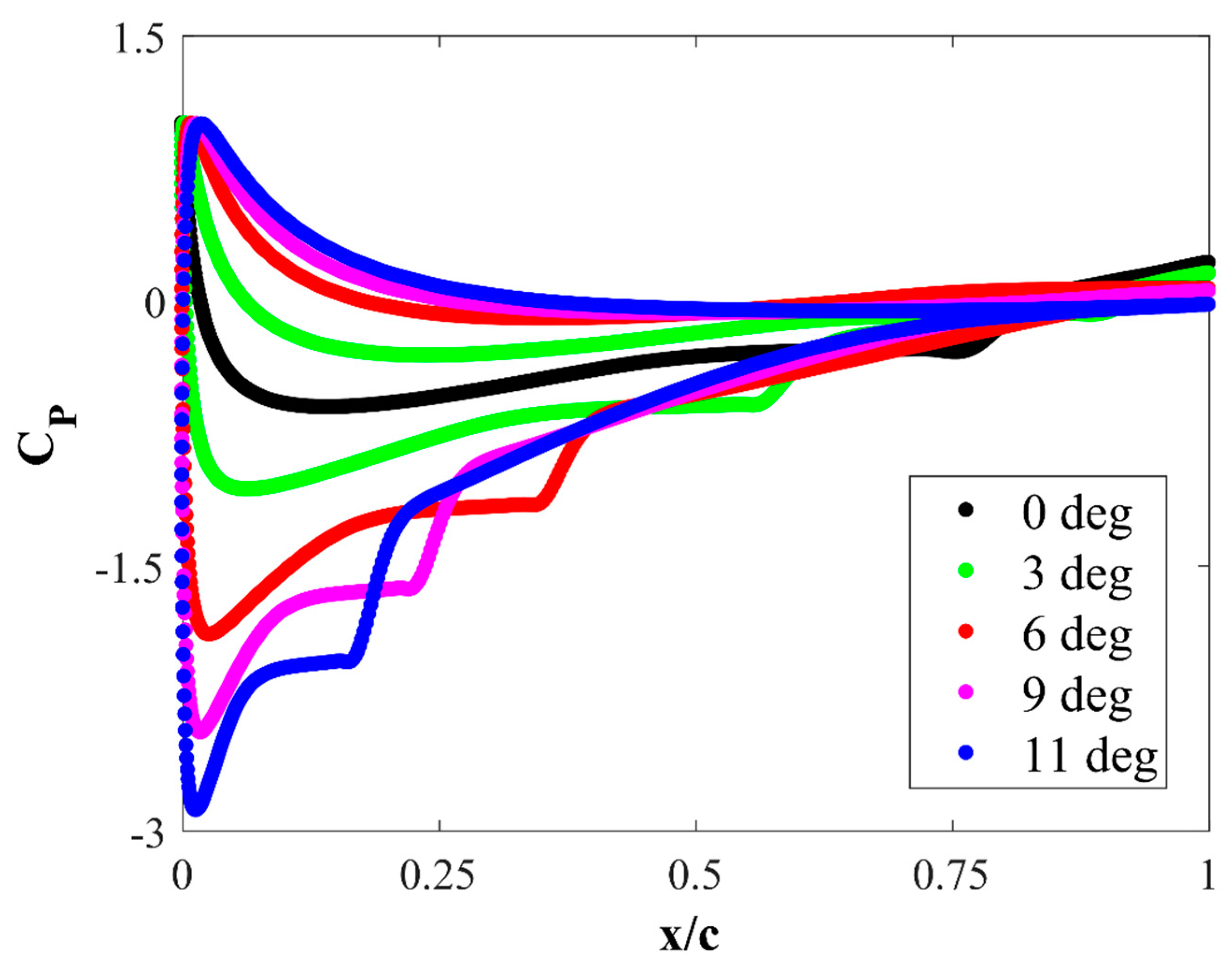
3.2. Pressure Distributions
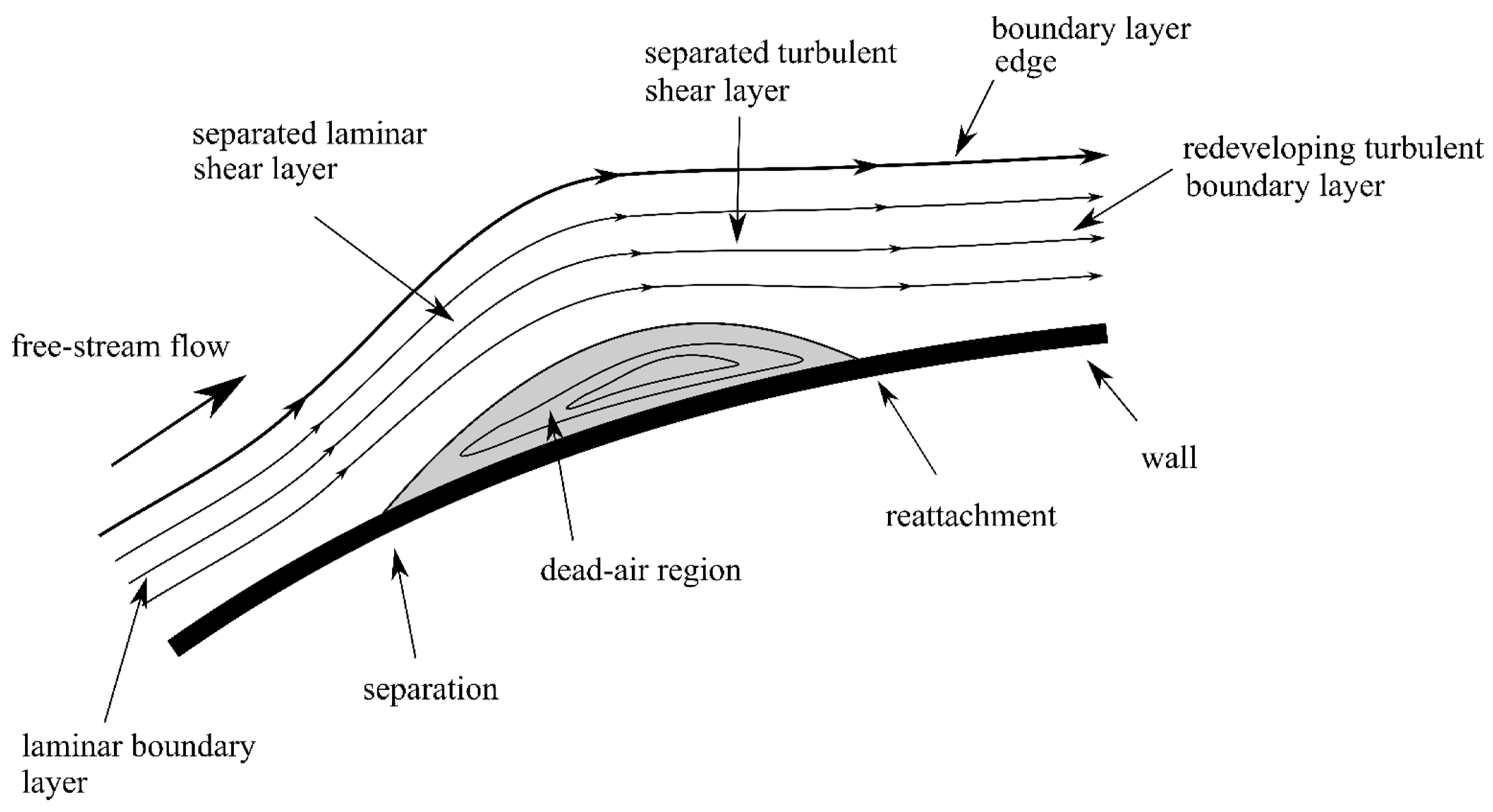
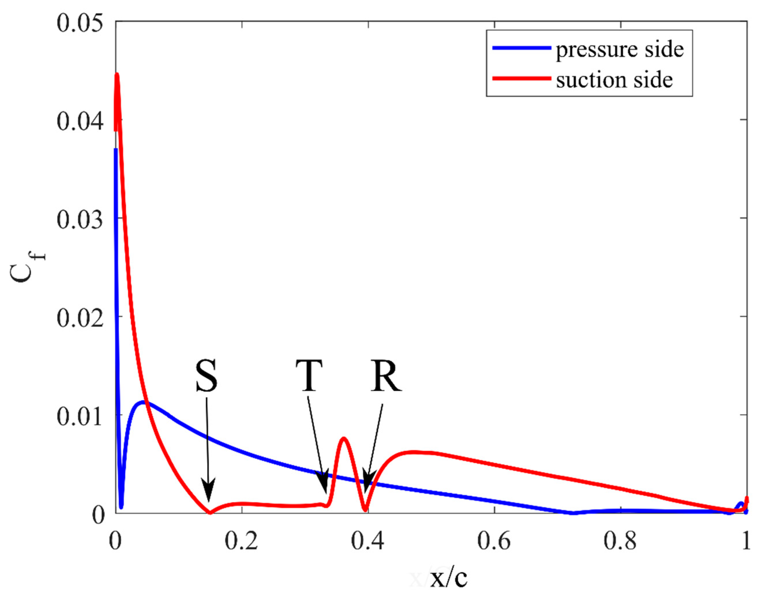
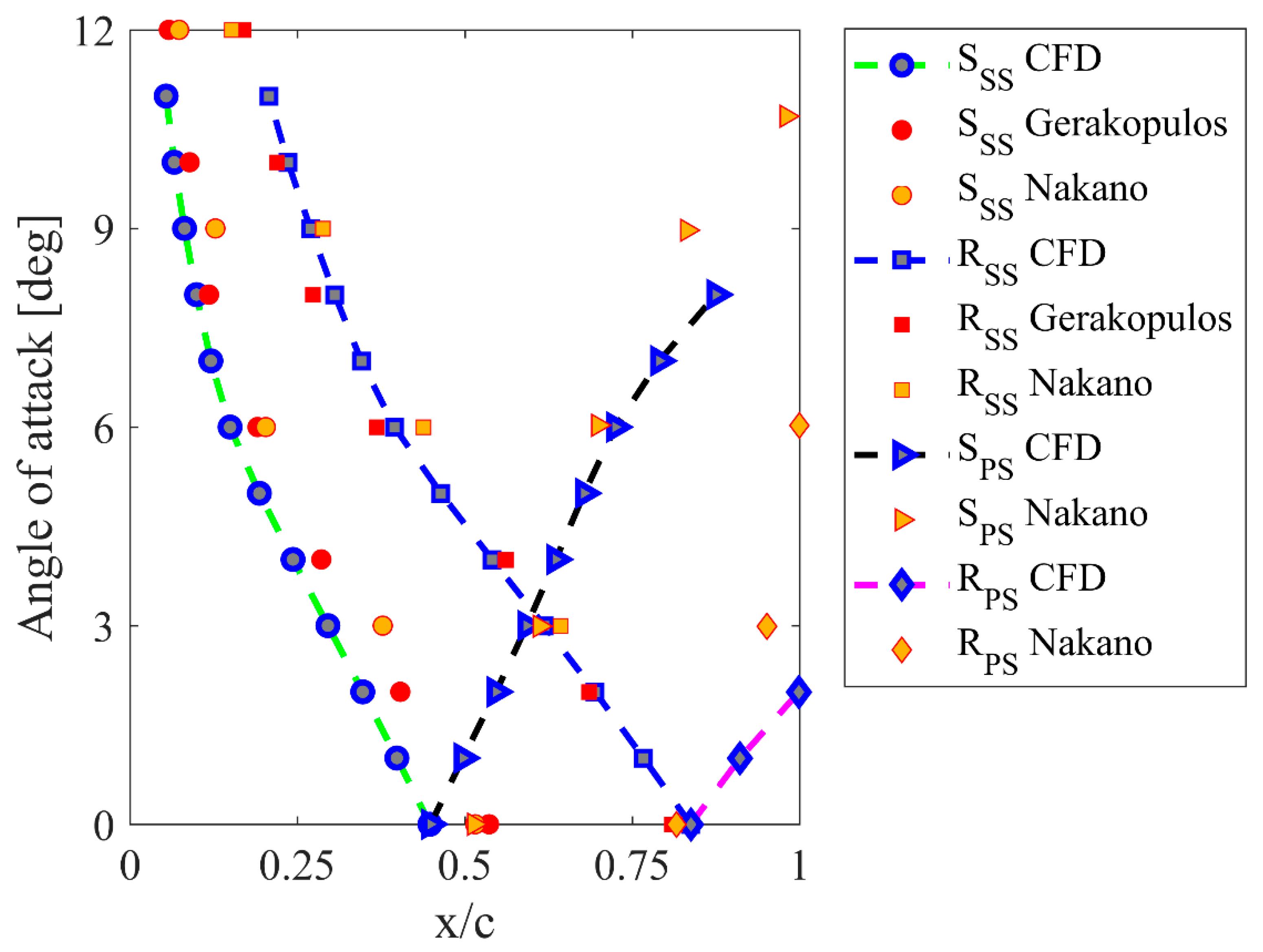
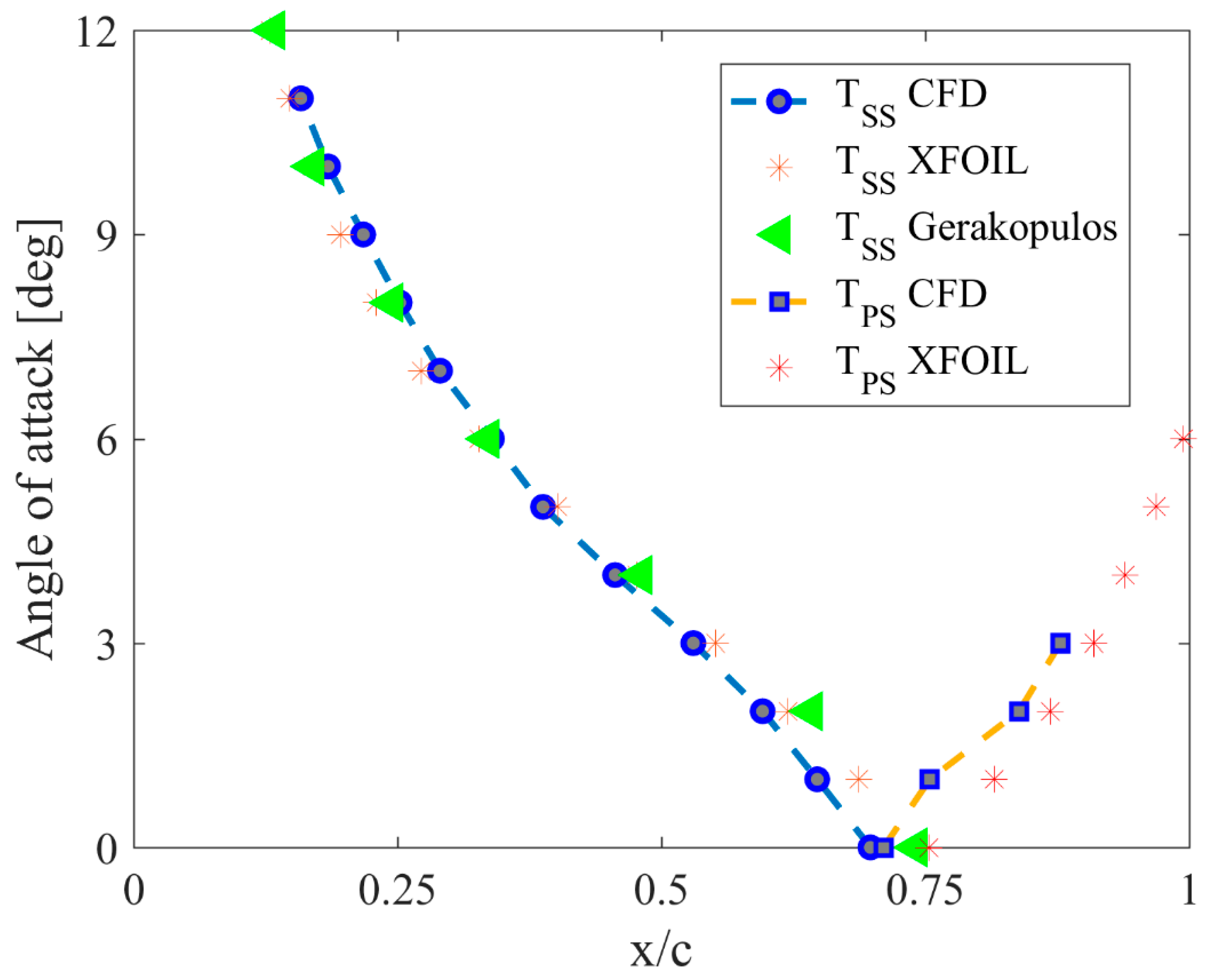
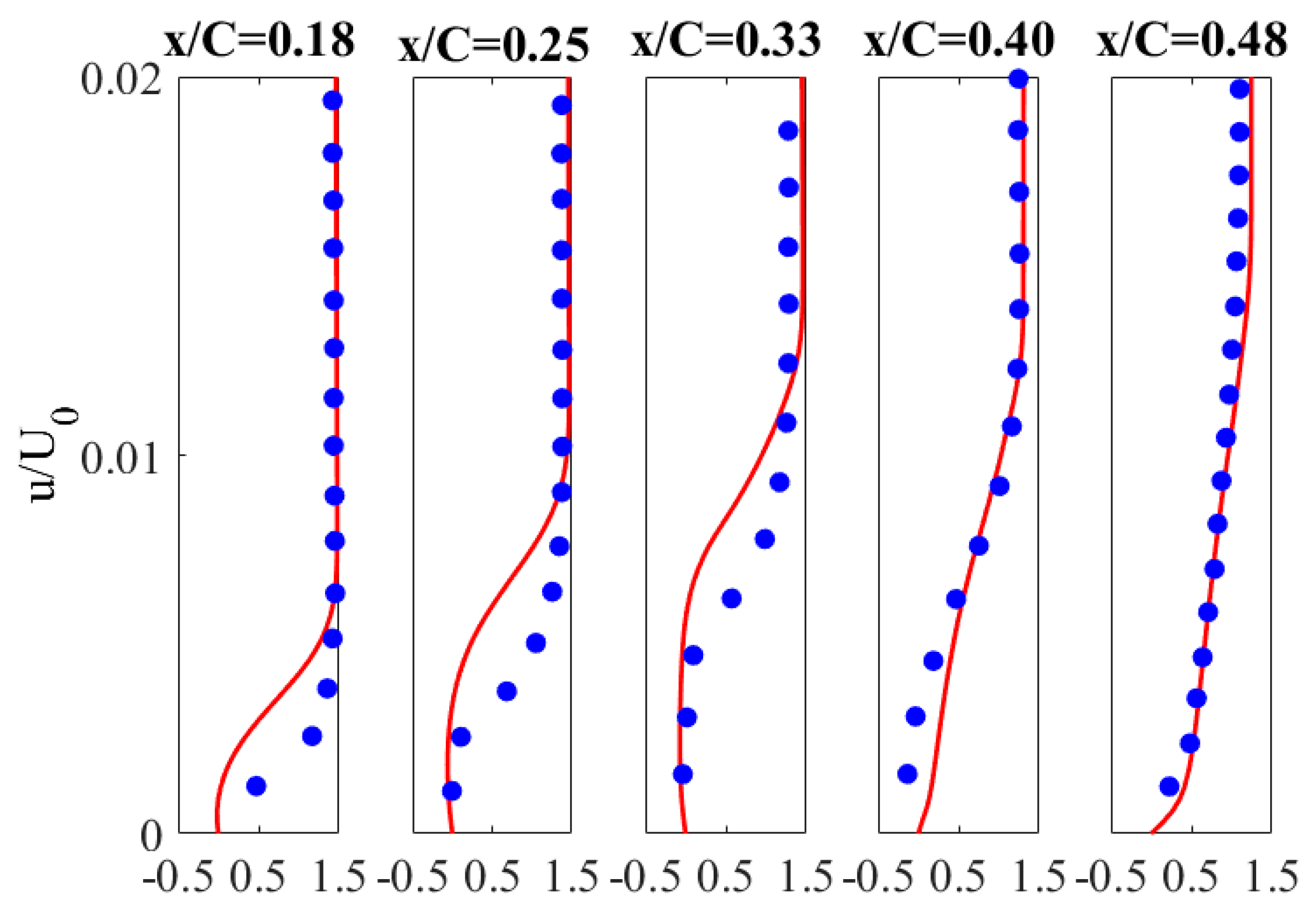
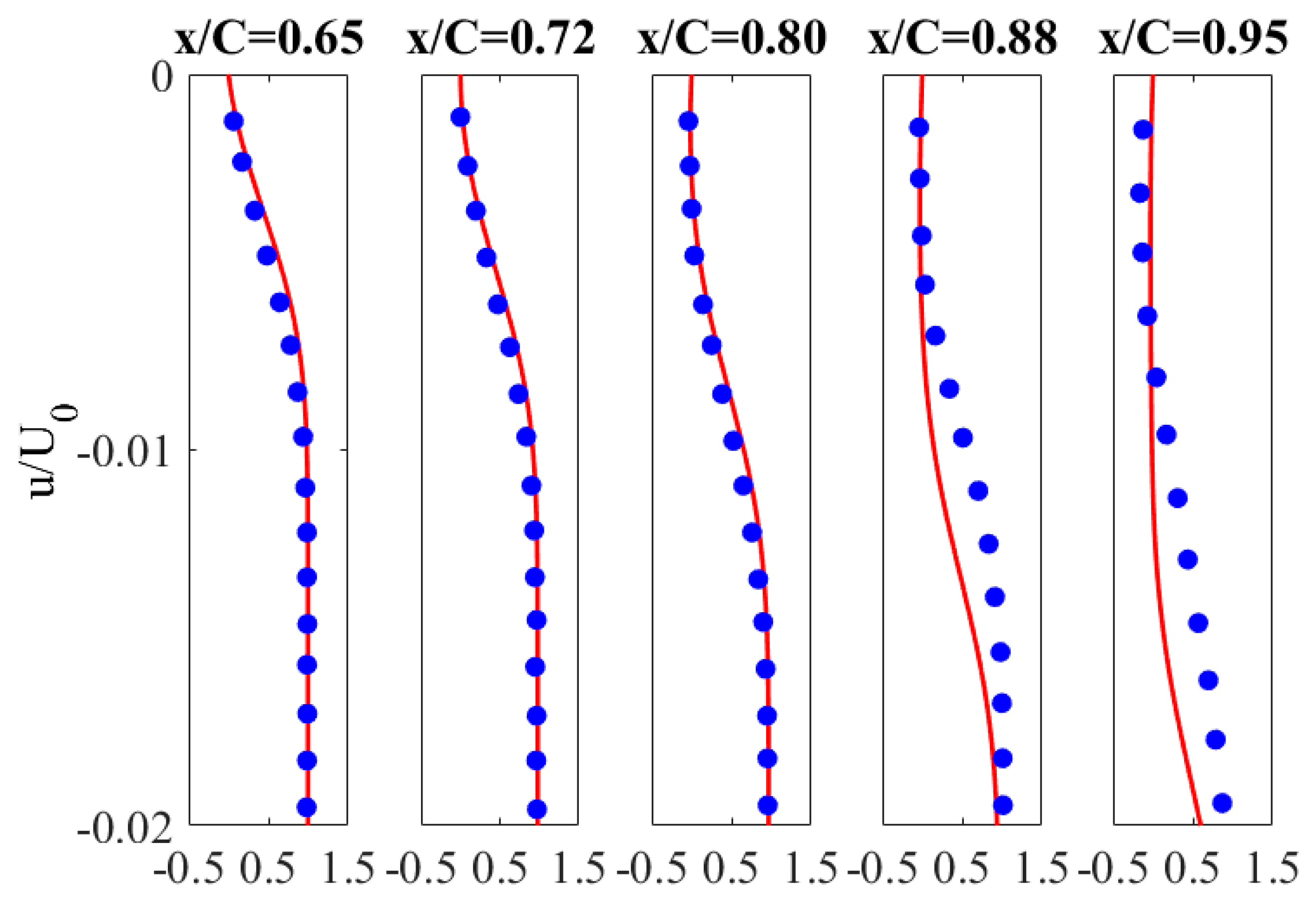
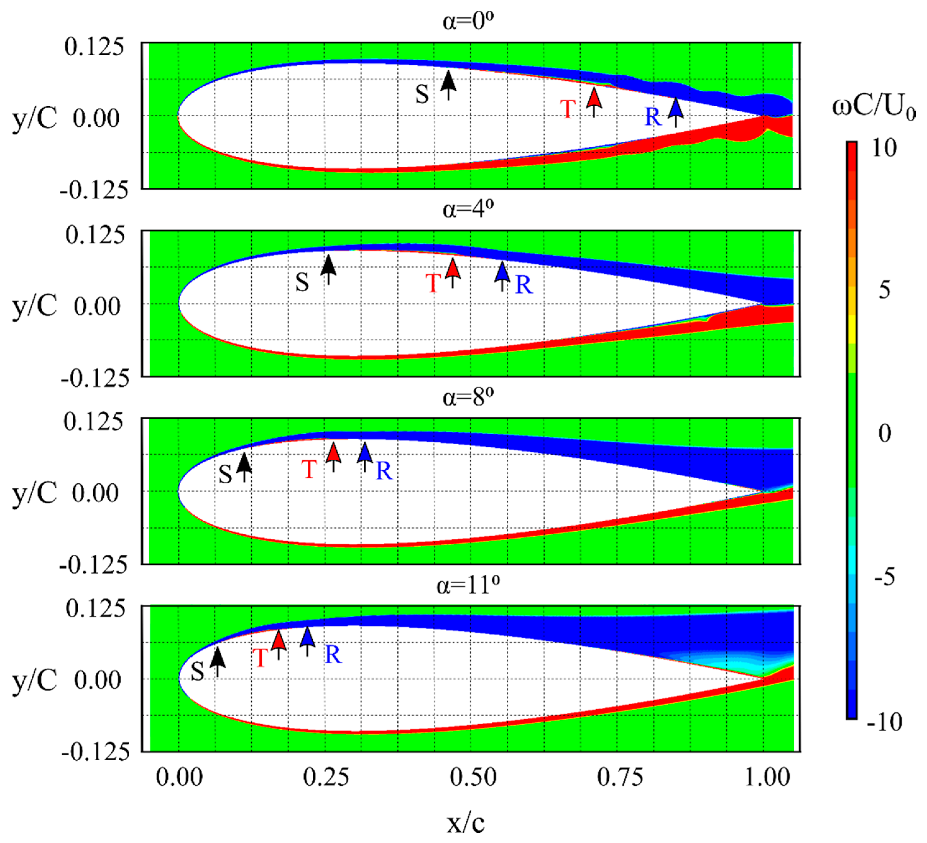
3.3. Laminar Separation Bubble Characteristics and Mean Velocity Distributions in the Near-Wall Region
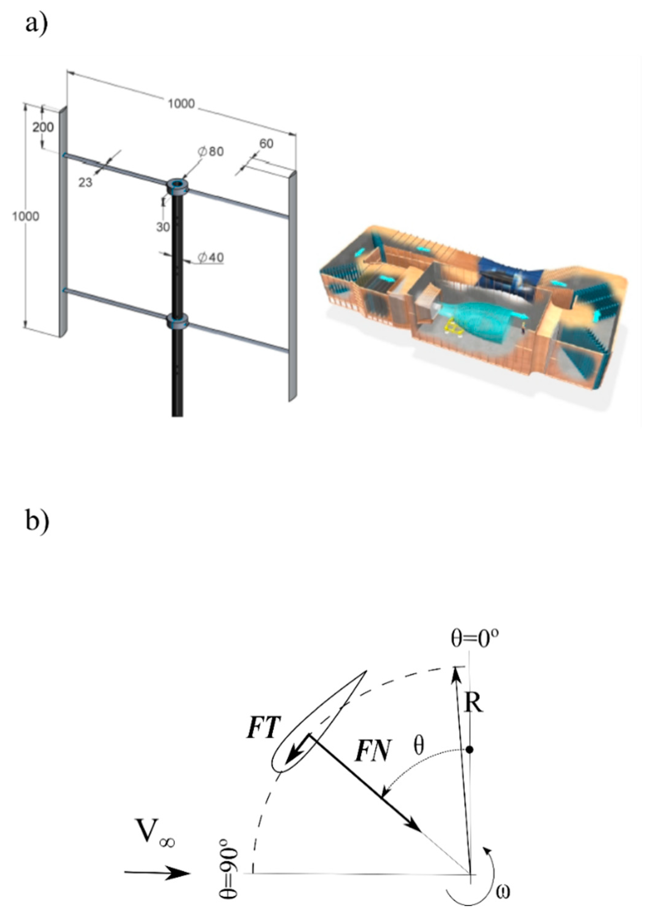
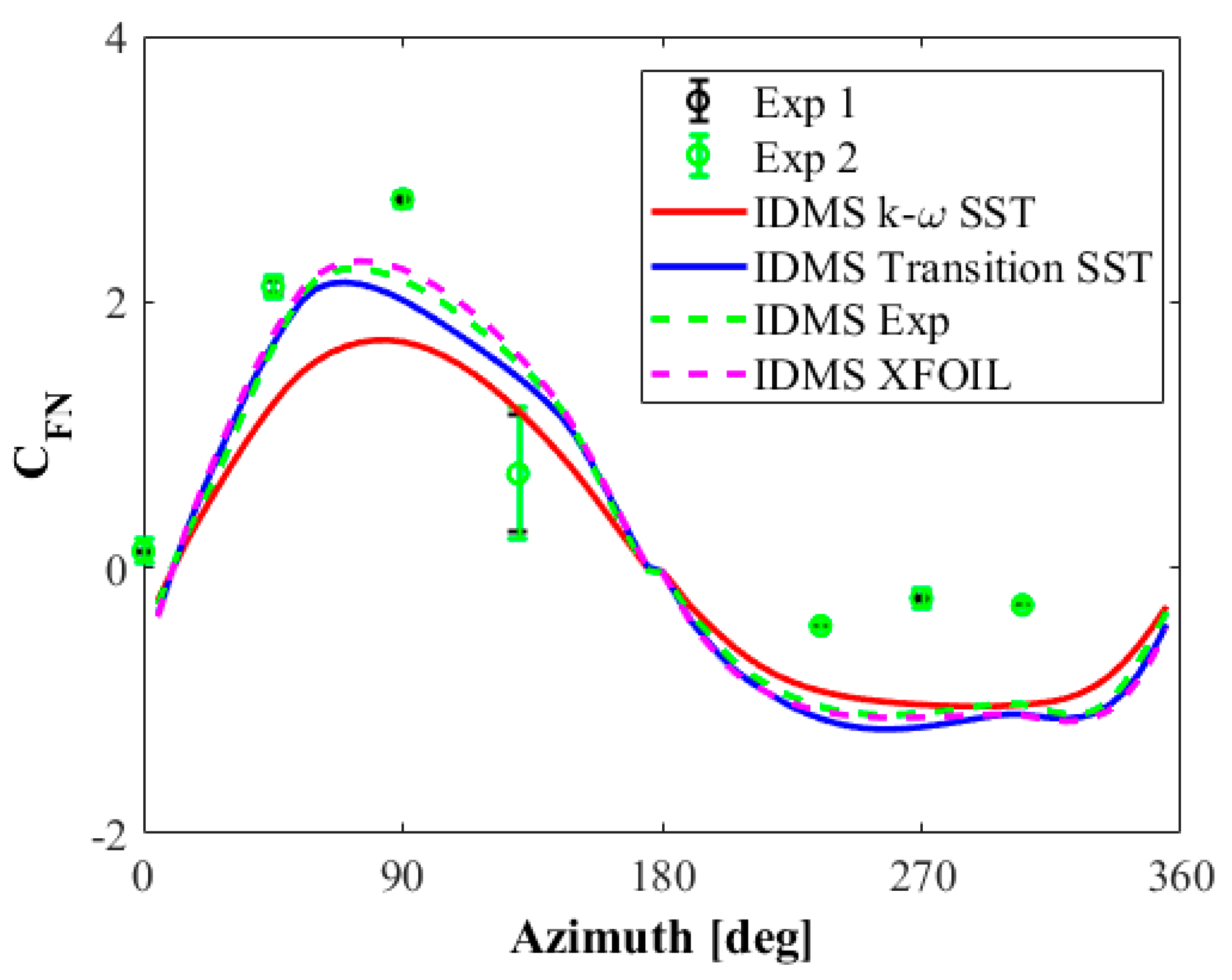
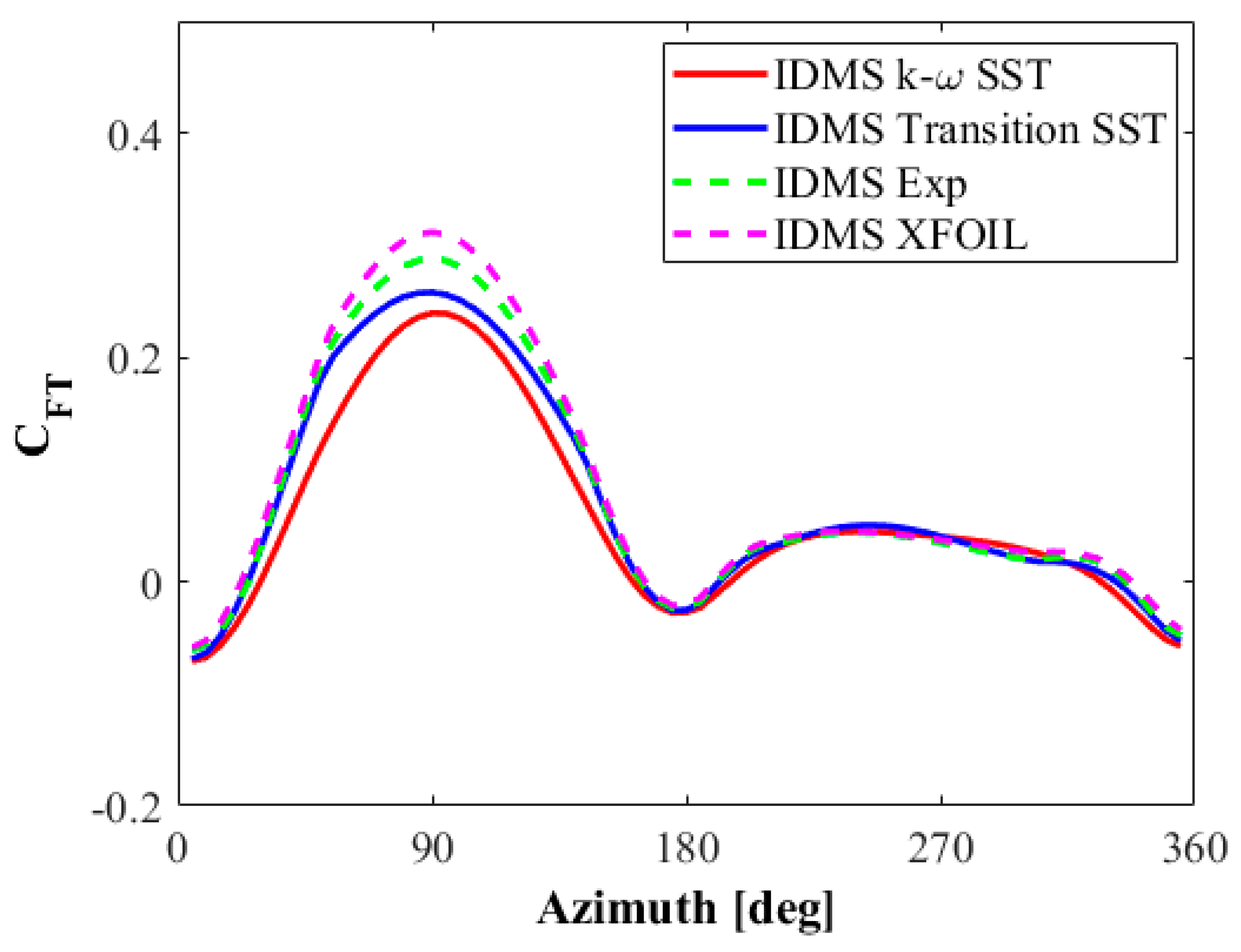
4. Vertical Axis Wind Turbine Test Case
- CFD polar calculated using the SST model
- CFD polar calculated using the transitional SST model
- Polar obtained from the measurement of Timmer
- Polar data calculated using XFOIL with the critical amplification factor of N = 9.0.
5. Conclusions
- This paper continues the research carried out by Królak and presented in his thesis [72]. Królak used the same geometric model, the Reynolds-averaged Navier–Stokes (RANS) technique, and the Transition SST turbulence model. The results of the aerodynamic force coefficients and the pressure distributions were burdened with considerable numerical errors. In particular, there were considerable nonphysical oscillations around the transition location. This article shows that the numerical calculations of the NACA airfoil should be carried out in a transient mode. Langtry reported similarly in many of the analyzed test cases [51].
- The analysis of the aerodynamic properties of the NACA 0018 airfoil was possible only in the transient mode, which, however, significantly increased the computational effort and increased the simulation time of a single case.
- The use of the Transition SST model made it possible to find two regions on the characteristic that were characterized by two aerodynamic derivatives in the range up to the critical angle of attack, instead of one derivative, as predicted by the two-equation k-ω SST turbulence model. The first region was found up to an angle of attack of 6 degrees, and the second up to 11 degrees.
- The values of the aerodynamic derivatives corresponded quite well with the experimental data; however, above the angle of attack equal to 6 degrees, the results of the lift coefficient were underestimated compared to the experimental data. This is probably due to the 3D effects, which were not included in these numerical studies.
- The Transition SST approach predicted the minimum drag coefficient by far the most accurately in comparison to the experimental results.
- The Transition SST model relatively accurately estimated the location and size of the laminar separation bubble on the suction surface of the airfoil. The average relative error in the localization of the separation point for the entire range of the investigated angles of attack was 22% compared to the experiment of Gerakopulos [21]. The reattachment point was estimated much more precisely; the mean relative error was 5.5%. This gives there was a mean relative error of 22% in estimating the length of the laminar separation bubble. The underestimation of the separation point of the laminar boundary layer in the CFD analysis compared to the experiment may be the result of using a two-dimensional numerical model that neglected the evolution of vortex structures in the direction of the span [66]. Another likely reason is that the model was not calibrated for this particular issue. The original formulation of the Transition SST model was calibrated for the small separation bubbles visible in the machines [2].
- The use of the more expensive turbulence model, i.e., the Transition SST model, to calculate the airfoil characteristics of the NACA 0018, however, significantly improved the normal force distribution of the Darrieus wind turbine rotor calculated using simplified aerodynamic methods.
Author Contributions
Funding
Institutional Review Board Statement
Informed Consent Statement
Data Availability Statement
Acknowledgments
Conflicts of Interest
Nomenclature
| chord length | |
| drag coefficient | |
| averaged drag coefficient | |
| skin friction coefficient | |
| normal force coefficient | |
| lift coefficient | |
| averaged lift coefficient | |
| tangential force coefficient | |
| static pressure coefficient | |
| normal force | |
| tangential force | |
| R | reattachment point; rotor radius of the Darrieus wind turbine rotor |
| the radius of the front edge of the domain size | |
| S | separation point |
| SD | standard deviation |
| T | transition point |
| free stream wind velocity (in NACA 0018 simulations) | |
| free stream wind velocity (in VAWT calculations) | |
| angle of attack | |
| dynamic viscosity | |
| kinematic viscosity | |
| air density | |
| wind turbine rotational speed; vorticity |
References
- Lin, J.M.; Pauley, L.L. Low-Reynolds-number separation on an airfoil. AIAA J. 1996, 34, 1570–1577. [Google Scholar] [CrossRef]
- Choudhry, A.; Arjomandi, M.; Kelso, R. A study of long separation bubble on thick airfoils and its consequent effects. Int. J. Heat Fluid Flow 2015, 52, 84–96. [Google Scholar] [CrossRef]
- Jimenez, P.; Lichota, P.; Agudelo, D.; Rogowski, K. Experimental validation of total energy control system for UAVs. Energies 2020, 13, 14. [Google Scholar] [CrossRef] [Green Version]
- Nakano, T.; Fujisawa, N.; Oguma, Y.; Takagi, Y.; Lee, S. Experimental study on flow and noise characteristics of NACA0018 airfoil. J. Wind. Eng. Ind. Aerodyn. 2007, 95, 511–531. [Google Scholar] [CrossRef]
- Zhang, W.; Hain, R.; Kähler, C.J. Scanning PIV investigation of the laminar separation bubble on a SD7003 airfoil. Exp. Fluids 2008, 45, 725–743. [Google Scholar] [CrossRef]
- Lissaman, P. Low-Reynolds-number airfoils. Annu. Rev. Fluid Mech. 1983, 15, 223–239. [Google Scholar] [CrossRef]
- Ol, M.V.; McAuliffe, B.R.; Hanff, E.S.; Scholz, U.; Kähler, C. Comparison of laminar separation bubble measurements on a low Reynolds number airfoil in three facilities. AIAA J. 2005, 5149. [Google Scholar] [CrossRef]
- Rezaeiha, A.; Kalkman, I.; Montazeri, H.; Blocken, B. Effect of the shaft on the aerodynamic performance of urban vertical axis wind turbines. Energy Convers. Manag. 2017, 149, 616–630. [Google Scholar] [CrossRef]
- Tummala, A.; Velamati, R.K.; Sinha, D.K.; Indraja, V.; Krishna, V.H. A review on small scale wind turbines. Renew. Sustain. Energy Rev. 2016, 56, 1351–1371. [Google Scholar] [CrossRef]
- Müller, G.; Chavushoglu, M.; Kerri, M.; Tsuzaki, T. A resistance type vertical axis wind turbine for building integration. Renew. Energy 2017, 111, 803–814. [Google Scholar] [CrossRef] [Green Version]
- Bangga, G.; Dessoky, A.; Wu, Z.; Rogowski, K.; Hansen, M.O.L. Accuracy and consistency of CFD and engineering models for simulating vertical axis wind turbine loads. Energy 2020, 206, 118087. [Google Scholar] [CrossRef]
- Rogowski, K.; Hansen, M.O.L.; Bangga, G. Performance Analysis of a H-Darrieus Wind Turbine for a Series of 4-Digit NACA Airfoils. Energies 2020, 13, 3196. [Google Scholar] [CrossRef]
- Cheng, Z.; Madsen, H.A.; Gao, Z.; Moan, T. Effect of the number of blades on the dynamics of floating straight-bladed vertical axis wind turbines. Renew. Energy 2017, 101, 1285–1298. [Google Scholar] [CrossRef]
- Bedon, G.; Schmidt Paulsen, U.; Madsen, H.A.; Belloni, F.; Raciti Castelli, M.; Benini, E. Computational assessment of the DeepWind aerodynamic performance with different blade and airfoil configurations. Appl. Energy 2017, 185, 1100–1108. [Google Scholar] [CrossRef]
- Cheng, Z.; Madsen, H.A.; Gao, Z.; Moan, T. A fully coupled method for numerical modeling and dynamic analysis of floating vertical axis wind turbines. Renew. Energy 2017, 107, 604–619. [Google Scholar] [CrossRef]
- Goude, A.; Aġren, O. Numerical simulation of a farm of vertical axis marine current turbines. In Proceedings of the ASME 2010 29th International Conference on Ocean, Offshore and Arctic Engineering, Shanghai, China, 6–11 June 2010; pp. 335–344. [Google Scholar] [CrossRef]
- Bangga, G.; Dessoky, A.; Lutz, T.; Krämer, E. Improved double-multiple-streamtube approach for H-Darrieus vertical axis wind turbine computations. Energy 2019, 182, 673–688. [Google Scholar] [CrossRef]
- Rainbird, J.M.; Bianchini, A.; Balduzzi, F.; Peiró, J.; Graham, J.M.R.; Ferrara, G.; Ferrari, L. On the influence of virtual camber effect on airfoil polars for use in simulations of Darrieus wind turbines. Energy Convers. Manag. 2015, 106, 373–384. [Google Scholar] [CrossRef]
- Melani, P.F.; Balduzzi, F.; Ferrara, G.; Bianchini, A. An Annotated Database of Low Reynolds Aerodynamic Coefficients for the NACA0018 Airfoil. AIP Conf. Proc. 2019, 2191, 020110. [Google Scholar] [CrossRef]
- Paraschivoiu, I. Wind Turbine Design with Emphasis on Darrieus Concept; Presses Internationales Polytechnique: Montréal, QC, Canada, 2009. [Google Scholar]
- Gerakopulos, R.; Boutilier, M.S.H.; Yarusevych, S. Aerodynamic Characterization of a NACA 0018 Airfoil at Low Reynolds Numbers. In Proceedings of the AIAA 2010-4629, 40th Fluid Dynamics Conference and Exhibit, Chicago, IL, USA, 28 June–1 July 2010. [Google Scholar] [CrossRef]
- Rogowski, K.; Maroński, R.; Hansen, M.O.L. Steady and unsteady analysis of NACA 0018 airfoil in vertical-axis wind turbine. J. Theor. Appl. Mech. 2018, 51, 203–212. [Google Scholar] [CrossRef] [Green Version]
- Langtry, R.B.; Menter, F.R. Correlation-Based Transition Modeling for Unstructured Parallelized Computational Fluid Dynamics Codes. AIAA J. 2009, 47, 2894–2906. [Google Scholar] [CrossRef]
- Lichota, P.; Szulczyk, J.; Noreña, D.A.; Vallejo Monsalve, F.A. Power spectrum optimization in the design of multisine manoeuvre for identification purposes. J. Theor. Appl. Mech. 2017, 55, 1193–1203. [Google Scholar] [CrossRef]
- Lichota, P. Multi-Axis Inputs for Identification of a Reconfigurable Fixed-Wing UAV. Aerospace 2020, 7, 113. [Google Scholar] [CrossRef]
- Schlichting, H. Boundary Layer Theory, 7th ed.; McGraw-Hill, Inc.: New York, NY, USA, 1979. [Google Scholar]
- Genç, M.S.; Karasu, I.; Açıkel, H.H.; Akpolat, M.T. Low Reynolds Number Flows and Transition; Gençm, S., Ed.; InTech-Open Access: Rijeka, Croatia, 2012; pp. 1–28. [Google Scholar]
- Abu-Ghannam, B.J.; Shaw, R. Natural transition of boundary layers—the effects of turbulence, pressure gradient, and flow history. J. Mech. Eng. Sci. 1980, 22, 213–228. [Google Scholar] [CrossRef]
- Morkovin, M.V. On the Many Faces of Transition; Wells, C.S., Ed.; Viscous Drag Reduction; Plenum Press: New York, NY, USA, 1969; pp. 1–31. [Google Scholar]
- Kubacki, S.; Jonak, P.; Dick, E. Evaluation of an algebraic model for laminar-to-turbulent transition on secondary flow loss in a low-pressure turbine cascade with an end wall. Int. J. Heat Fluid Flow 2019, 77, 98–112. [Google Scholar] [CrossRef]
- Kubacki, S.; Dick, E. An algebraic model for bypass transition in turbomachinery boundary layer flows. Int. J. Heat Fluid Flow 2019, 58, 68–83. [Google Scholar] [CrossRef]
- Mayle, R.E. The Role of Laminar-Turbulent Transition in Gas Turbine Engines. J. Turbomach. 1991, 113, 509–537. [Google Scholar] [CrossRef]
- Mayle, R.E.; Schulz, A. The Path to Predicting Bypass Transition. In Proceedings of the ASME 1996 International Gas Turbine and Aeroengine Congress and Exhibition, Turbomachinery, Birmingham, UK, 10–13 June 1996; Volume 1. V001T01A065. [Google Scholar] [CrossRef] [Green Version]
- Tani, I. Low Speed Flows Involving Bubble Separations. Prog. Aerosp. Sci. 1964, 5, 70–103. [Google Scholar] [CrossRef]
- Swift, K.M. An Experimental Analysis of the Laminar Separation Bubble at Low Reynolds Numbers. Master’s Thesis, University of Tennessee, Knoxville, TN, USA, 2009. [Google Scholar]
- Li, Q.; Maeda, T.; Kamada, Y.; Murata, J.; Kawabata, T.; Shimizu, K.; Ogasawara, T.; Nakai, A.; Kasuya, T. Wind tunnel and numerical study of a straight-bladed vertical axis wind turbine in three-dimensional analysis (Part I: For predicting aerodynamic loads and performance). Energy 2016, 106, 443–452. [Google Scholar] [CrossRef]
- Roh, S.C.; Kang, S.H. Effects of a blade profile, the Reynolds number, and the solidity on the performance of a straight bladed vertical axis wind turbine. J. Mech. Sci. Technol. 2013, 27, 3299–32307. [Google Scholar] [CrossRef]
- Mohamed, M.H. Performance investigation of H-rotor Darrieus turbine with new airfoil shapes. Energy 2012, 47, 522–530. [Google Scholar] [CrossRef]
- Islam, M.; Ting, D.S.K.; Fartaj, A. Desirable airfoil features for smaller-capacity straight-bladed VAWT. Wind Eng. 2007, 31, 165–196. [Google Scholar] [CrossRef]
- Jacobs, E.N.; Sherman, A. Airfoil Section Characteristics as Affected by Variations of the Reynolds Number. NACA Rep. 1937, 586, 227–267. [Google Scholar]
- Timmer, W.A. Two-Dimensional Low-Reynolds Number Wind Tunnel Results for Airfoil NACA 0018. Wind. Eng. 2008, 32, 525–537. [Google Scholar] [CrossRef] [Green Version]
- Laneville, A.; Vittecoq, P. Dynamic stall: The case of the vertical axis wind turbine. J. Sol. Energy Eng. 1986, 108, 141–145. [Google Scholar] [CrossRef]
- Sheldahl, R.E.; Klimas, P.C. Aerodynamic Characteristics of Seven Symmetrical Airfoil Sections through 180-Degree Angle of Attack for Use in Aerodynamic Analysis of Vertical Axis Wind Turbines; Technical Report SAND80-2114; Sandia National Labs: Albuquerque, NM, USA, 1981.
- Boutilier, M.S.H.; Yarusevych, S. Parametric study of separation and transition characteristics over an airfoil at low Reynolds numbers. Exp. Fluids 2012, 52, 1491–1506. [Google Scholar] [CrossRef]
- Claessens, M.C. The Design and Testing of Airfoils in Small Vertical Axis Wind Turbines. Master’s Thesis, TU Delft, Delft, The Netherlands, 2006. [Google Scholar]
- Bianchini, A.; Balduzzi, F.; Rainbird, J.M.; Peiro, J.; Graham, J.M.R.; Ferrara, G.; Ferrari, L. An Experimental and Numerical Assessment of Airfoil Polars for Use in Darrieus Wind Turbines—Part II: Post-stall Data Extrapolation Methods. J. Eng. Gas. Turbine Power 2016, 138. [Google Scholar] [CrossRef]
- Kątski, B.; Rogowski, K. Analysis of the Aerodynamic Properties of the NACA 0018 Airfoil in the Range of Low Reynolds Numbers; Krzysztof, S., Ed.; Mechanics in Aviation ML-XIX 2020; ITWL and PTMTS: Warsaw, Poland, 2020; Volume 1, pp. 57–65. [Google Scholar]
- Rogowski, K. Numerical studies on two turbulence models and a laminar model for aerodynamics of a vertical-axis wind turbine. J. Mech. Sci. Technol. 2018, 32, 2079–2088. [Google Scholar] [CrossRef]
- Rogowski, K.; Hansen, M.O.L.; Lichota, P. 2-D CFD Computations of the Two-Bladed Darrieus-Type Wind Turbine. J. Appl. Fluid Mech. 2018, 11, 835–845. [Google Scholar] [CrossRef]
- Divakaran, U.; Ramesh, A.; Mohammad, A.; Velamati, R.K. Effect of Helix Angle on the Performance of Helical Vertical Axis Wind Turbine. Energies 2021, 14, 393. [Google Scholar] [CrossRef]
- Langtry, R.B. A Correlation-Based Transition Model using Local Variables for Unstructured Parallelized CFD Codes. Ph.D Thesis, Universität Stuttgart, Stuttgart, Germany, 2006. [Google Scholar] [CrossRef]
- Smith, A.M.O.; Gamberoni, N. Transition, Pressure Gradient and Stability Theory; Douglas Aircraft Company, El Segundo Division: Los Angeles, CA, USA, 1956. [Google Scholar]
- Rogowski, K.; Hansen, M.O.L.; Maroński, R.; Lichota, P. Scale Adaptive Simulation Model for the Darrieus Wind Turbine. J. Phys. Conf. Ser. 2016, 753, 022050. [Google Scholar] [CrossRef]
- Bianchini, A.; Balduzzi, F.; Rainbird, J.M.; Peiro, J.; Graham, J.M.R.; Ferrara, G.; Ferrari, L. An Experimental and Numerical Assessment of Airfoil Polars for Use in Darrieus Wind Turbines—Part I: Flow Curvature Effects. J. Eng. Gas Turbine Power 2016, 138, 032602. [Google Scholar] [CrossRef]
- Guo, Z.; Fletcher, D.F.; Haynes, B.S. Implementation of a height function method to alleviate spurious currents in CFD modelling of annular flow in microchannels. Appl. Math. Model. 2015, 39, 4665–4686. [Google Scholar] [CrossRef]
- ANSYS, Inc. ANSYS Fluent Theory Guide, Release 19.0.; ANSYS, Inc.: Canonsburg, PA, USA.
- Menter, F. Two-equation eddy-viscosity turbulence models for engineering applications. AIAA J. 1994, 32, 1598–1605. [Google Scholar] [CrossRef] [Green Version]
- Goetten, F.; Finger, D.F.; Marino, M.; Bil, C. A review of guidelines and best practices for subsonic aerodynamic simulations using RANS CFD. In Proceedings of the Asia-Pacific International Symposium on Aerospace Technology (APISAT), Gold Coast, Australia, 4–6 December 2019. [Google Scholar]
- Schlipf, M.; Tismer, A.; Riedelbauch, S. On the application of hybrid meshes in hydraulic machinery CFD simulations. IOP Conf. Ser. Earth Environ. Sci. 2016, 49, 062013. [Google Scholar] [CrossRef] [Green Version]
- Schmidt, S.; Thiele, F. Detached Eddy Simulation of Flow around A-Airfoil. Flow Turbul. Combust. 2003, 71, 261–278. [Google Scholar] [CrossRef]
- Bangga, G.; Lutz, T.; Dessoky, A.; Krämer, E. Unsteady Navier-Stokes studies on loads, wake and dynamic stall characteristics of a two-bladed vertical axis wind turbine. J. Renew. Sustain. Energy 2017, 9, 053303. [Google Scholar] [CrossRef] [Green Version]
- Marchman, J.F. Aerodynamic Testing at Low Reynolds Numbers. J. Aircr. 1987, 24, 107–114. [Google Scholar] [CrossRef]
- Laitone, E.V. Wind tunnel tests of wings at Reynolds numbers below 70,000. Exp. Fluids 1997, 23, 405–409. [Google Scholar] [CrossRef]
- Du, L. Numerical and Experimental Investigations of Darrieus Wind Turbine Start-up and Operation. Ph.D. Thesis, Durham University, Durham, UK, 2016. [Google Scholar]
- Yao, J.; Yuan, W.; Wang, J.; Xie, J.; Zhou, H.; Peng, M.; Sun, Y. Numerical simulation of aerodynamic performance for two dimensional wind turbine airfoils. Procedia Eng. 2012, 31, 80–86. [Google Scholar] [CrossRef] [Green Version]
- Istvan, M.S.; Yarusevych, S. Effects of free-stream turbulence intensity on transition in a laminar separation bubble formed over an airfoil. Exp. Fluids 2018, 59, 1–21. [Google Scholar] [CrossRef]
- Tescione, G.; Ragni, D.; He, C.; Ferreira, C.J.S.; van Bussel, G.J.W. Near wake flow analysis of a vertical axis wind turbine by stereoscopic particle image velocimetry. Renew. Energy 2014, 70, 47–61. [Google Scholar] [CrossRef]
- Castelein, D.; Ragni, D.; Tescione, G.; Ferreira, C.J.S.; Gaunaa, M. Creating a benchmark of Vertical Axis Wind Turbines in Dynamic Stall for validating numerical models. In Proceedings of the 33rd Wind Energy Symposium, AIAA SciTech, AIAA 2015-0723, Kissimmee, FL, USA, 5–9 January 2015. [Google Scholar] [CrossRef]
- Paraschivoiu, I. Double-multiple streamtube model for studying vertical-axis wind turbines. J. Propul. Power 1988, 4, 370–377. [Google Scholar] [CrossRef]
- Bangga, G. Comparison of Blade Element Method and CFD Simulations of a 10 MW Wind Turbine. Fluids 2018, 3, 73. [Google Scholar] [CrossRef] [Green Version]
- Strickland, J.H.; Webster, B.T.; Nguyen, T.A. Vortex Model of the Darrieus Turbine: An Analytical and Experimental Study. J. Fluids Eng. 1979, 101, 500–505. [Google Scholar] [CrossRef]
- Królak, G. Numerical Analysis of Aerodynamic Characteristics of the NACA 0018 Airfoil Used in the Darrieus Wind Turbines. Master’s Thesis, Warsaw University of Technology, Warsaw, Poland, 2021. [Google Scholar]


| Case | Number of Mesh Points on the Airfoil | Total Number of Mesh Elements |
|---|---|---|
| Case 1 | 208 | 175,440 |
| Case 2 | 416 | 350,880 |
| Case 3 | 830 | 700,400 |
| Case 4 | 1660 | 1,400,800 |
| Case 5 | 3320 | 2,767,600 |
| Case | Total Number of Mesh Elements | |||||
|---|---|---|---|---|---|---|
| Case 1 | 3.75c | 432,600 | 0.7457 | 0.0227 | ||
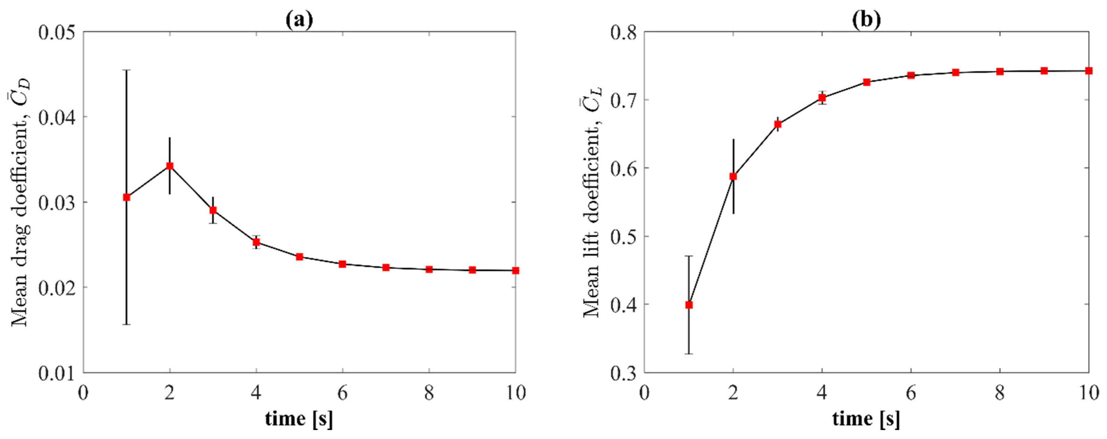
| Case 2 | 7.5c | 700,400 | 0.7425 | 0.0220 | 0.43 | 3.28 |
| Case 3 | 15c | 1,486,800 | 0.7412 | 0.0218 | 0.18 | 0.82 |
| Angle of Attack [deg] | ||
|---|---|---|
| 0 | 0.0168 (1.31 × 10⁻⁴) | 0.0004 (8.40 × 10⁻³) |
| 1 | 0.0170 (1.32 × 10⁻⁴) | 0.0960 (4.60 × 10⁻³) |
| 2 | 0.0178 (6.17 × 10⁻⁵) | 0.2120 (2.10 × 10⁻³) |
| 3 | 0.0187 (1.81 × 10⁻⁵) | 0.3500 (2.86 × 10⁻⁴) |
| 4 | 0.0197 (9.61 × 10⁻⁶) | 0.4959 (1.74 × 10⁻⁴) |
| 5 | 0.0208 (1.19 × 10⁻⁵) | 0.6339 (1.99 × 10⁻⁴) |
| 6 | 0.0220 (7.12 × 10⁻⁶) | 0.7425 (3.71 × 10⁻⁵) |
| 7 | 0.0229 (1.28 × 10⁻⁵) | 0.7750 (7.21 × 10⁻⁵) |
| 8 | 0.0246 (1.09 × 10⁻⁵) | 0.7833 (1.17 × 10⁻⁴) |
| 9 | 0.0270 (3.71 × 10⁻⁶) | 0.7984 (8.18 × 10⁻⁵) |
| 10 | 0.0306 (2.28 × 10⁻⁶) | 0.8279 (5.24 × 10⁻⁵) |
| 11 | 0.0357 (3.02 × 10⁻⁶) | 0.8606 (8.28 × 10⁻⁵) |
Publisher’s Note: MDPI stays neutral with regard to jurisdictional claims in published maps and institutional affiliations. |
© 2021 by the authors. Licensee MDPI, Basel, Switzerland. This article is an open access article distributed under the terms and conditions of the Creative Commons Attribution (CC BY) license (http://creativecommons.org/licenses/by/4.0/).
Share and Cite
Rogowski, K.; Królak, G.; Bangga, G. Numerical Study on the Aerodynamic Characteristics of the NACA 0018 Airfoil at Low Reynolds Number for Darrieus Wind Turbines Using the Transition SST Model. Processes 2021, 9, 477. https://0-doi-org.brum.beds.ac.uk/10.3390/pr9030477
Rogowski K, Królak G, Bangga G. Numerical Study on the Aerodynamic Characteristics of the NACA 0018 Airfoil at Low Reynolds Number for Darrieus Wind Turbines Using the Transition SST Model. Processes. 2021; 9(3):477. https://0-doi-org.brum.beds.ac.uk/10.3390/pr9030477
Chicago/Turabian StyleRogowski, Krzysztof, Grzegorz Królak, and Galih Bangga. 2021. "Numerical Study on the Aerodynamic Characteristics of the NACA 0018 Airfoil at Low Reynolds Number for Darrieus Wind Turbines Using the Transition SST Model" Processes 9, no. 3: 477. https://0-doi-org.brum.beds.ac.uk/10.3390/pr9030477