Self-Tuning Two Degree-of-Freedom Proportional–Integral Control System Based on Reinforcement Learning for a Multiple-Input Multiple-Output Industrial Process That Suffers from Spatial Input Coupling

Abstract

Proportional–integral–derivative (PID) control remains the primary choice for industrial process control problems. However, owing to the increased complexity and precision requirement of current industrial processes, a conventional PID controller may provide only unsatisfactory performance, or the determination of PID gains may become quite difficult. To address these issues, studies have suggested the use of reinforcement learning in combination with PID control laws. The present study aims to extend this idea to the control of a multiple-input multiple-output (MIMO) process that suffers from both physical coupling between inputs and a long input/output lag. We specifically target a thin film production process as an example of such a MIMO process and propose a self-tuning two-degree-of-freedom PI controller for the film thickness control problem. Theoretically, the self-tuning functionality of the proposed control system is based on the actor-critic reinforcement learning algorithm. We also propose a method to compensate for the input coupling. Numerical simulations are conducted under several likely scenarios to demonstrate the enhanced control performance relative to that of a conventional static gain PI controller.

1. Introduction

Control system synthesis for industrial processes has long attracted much research attention. However, the increased complexity and granularity of industrial processes make control system design difficult or intractable even for experienced engineers. Despite the sophistication of modern industrial processes, proportional–integral–derivative (PID) controllers remain the primary choice for industrial process control [1,2]. It was known that PID controllers could be applied to many control systems [3]. However, the broad application spectrum of PID controllers literally means that engineers have to find their own ways to tune their PID parameters to satisfy their performance objectives [4]. The adaptive and/or automatic tuning of the PID controller parameters was accordingly regarded as a course of development to provide feasible solutions to the problem.

Hägglund and Ȧström [4] proposed the auto-tuning scheme for PID controllers using artificially induced limit-cycle behavior. Papadopoulos et al. [5] proposed the automatic tuning of PID controllers based on the magnitude optimum criterion. Sarhadi et al. [6] applied an adaptive PID control for model reference adaptive control of an autonomous underwater vehicle. They derived a PID parameter tuning law based on the Lyapunov stability theory. These foregoing works were the prime examples of automatic PID gain tuning algorithms derived analytically. However, as their developments implicitly assumed that an accurate mathematical model of the plant was available, it might be difficult to apply their results directly to real-world targets.

The application of artificial intelligence to PID tuning is an alternative solution to the problem. Acosta et al. [7] applied the fuzzy logic algorithm to synthesize an expert PID controller based on the measurements of a closed-loop system. Solihin et al. [8] proposed the tuning of PID parameters with the particle swarm optimization algorithm proposed by Eberhart and Kennedy [9]. A PID controller for a temperature control problem of a heat exchanging device was proposed by Reddy and Balaji [10], whose gains were tuned by a genetic algorithm. These behavior based tuning methods can be applied to a wide range of targets, whereas it might require repetitive plant operations or simulations to determine a set of PID parameters.

The online auto-tuning of PID parameters has been developed in combination with neural networks. Han et al. [11] proposed a lateral tracking PID controller for their mobile wheeled robot. Their controller parameters were tuned with the help of a neural network and the back propagation algorithm. They used the Lyapunov stability theory to derive the network learning rules.

Recently, increasing interest in the application of reinforcement learning (RL) to control problems has been observed in the literature. RL itself has a structure that can directly issue control actions to a target process. Spielberg et al. [12] proposed the actor-critic Q-learning system for the control of a multiple-input multiple-output (MIMO) process model in which they introduced deep networks in the actor and critic separately. Zou et al. [13] used RL to formulate a deterministic greedy control policy for a thermal power generation plant. Fares et al. [14] formulated online actor-critic RL for the control of an active suspension system and showed that their controller outperformed the optimal PID controller.

Results have also been reported in the literature that uses RL for adaptive tuning of PID controller. The intrinsic advantage of RL in PID controller tuning lies in the “learn from experience” strategy. It introduces robustness to various uncertainties that the real processes might suffer, at the cost of transient unsuccessful attempts that might happen especially in the early stages of learning. Boubertakh et al. [15] proposed tuning of PD and PI controllers with RL. They formulated Takagi–Sugeno-type fuzzy controllers for robust inference. Wang et al. [16] proposed an adaptive RL PID control system with a radial basis function (RBF) network for the control of a complex, highly nonlinear single-input single-output (SISO) system. Sedighnizadeh and Rezazadeh [17] also proposed the use of RL in combination with an RBF network to synthesize an adaptive PID controller for a SISO wind turbine control problem.

The latest trend in the use of RL in PID tuning is the introduction of deep neural networks. Lee et al. [18] introduced a deep deterministic policy gradient algorithm to synthesize adaptive PID for a dynamic positioning system. Carlucho et al. [19] synthesized an adaptive deep reinforcement learning MIMO PID controller for model-free control of a mobile robot. These existing works offered a great enhancement to the conventional PID controllers whilst increasing robustness to uncertainties. However, most of the works targeted the control of SISO plants. Although some works treated the synthesis of the PID controller for MIMO plants, the number of inputs and/or outputs was typically limited to two or three.

In this paper, we attempt to synthesize an RL based PI controller with a feed-forward input for a thin film fabrication process that has fifteen inputs for controlling the thickness of the film and sixty-three thickness measurement outputs. We hereafter refer to our controller as the two-DOF PI controller. The objective of the film production process is to produce a film whose thickness should be as uniformly close as possible to its reference, and its perturbation should remain within the pre-specified tolerance for quality assurance of the product. This process is known to suffer from severe input coupling that originates from its mechanical design, as well as a large input lag. The tuning of the embedded PI controller parameters of the process is a difficult problem, and it requires elaborative manual tuning of highly experienced operators in the factory. We aim to provide an automatic self-tuning functionality to the PID controller in this study for automatic high-quality film production.

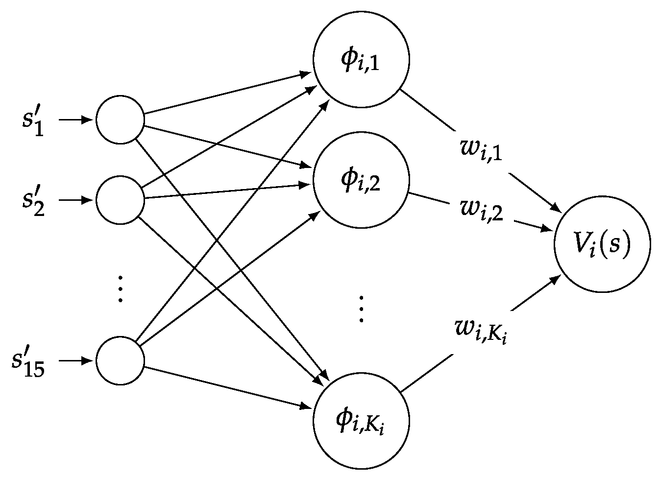
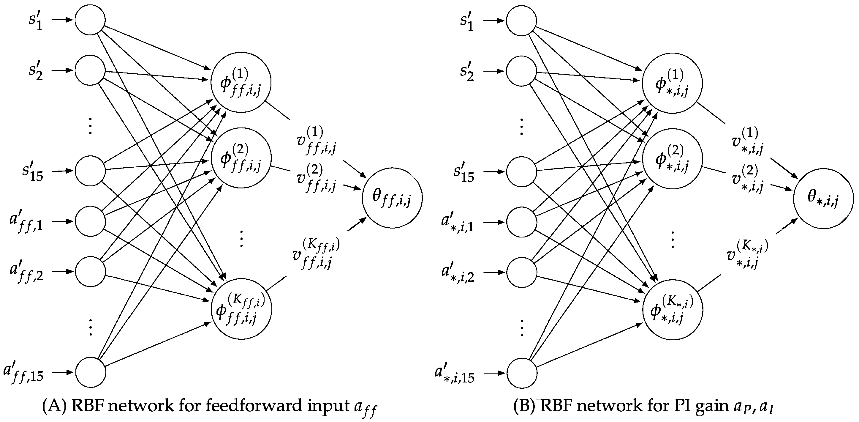
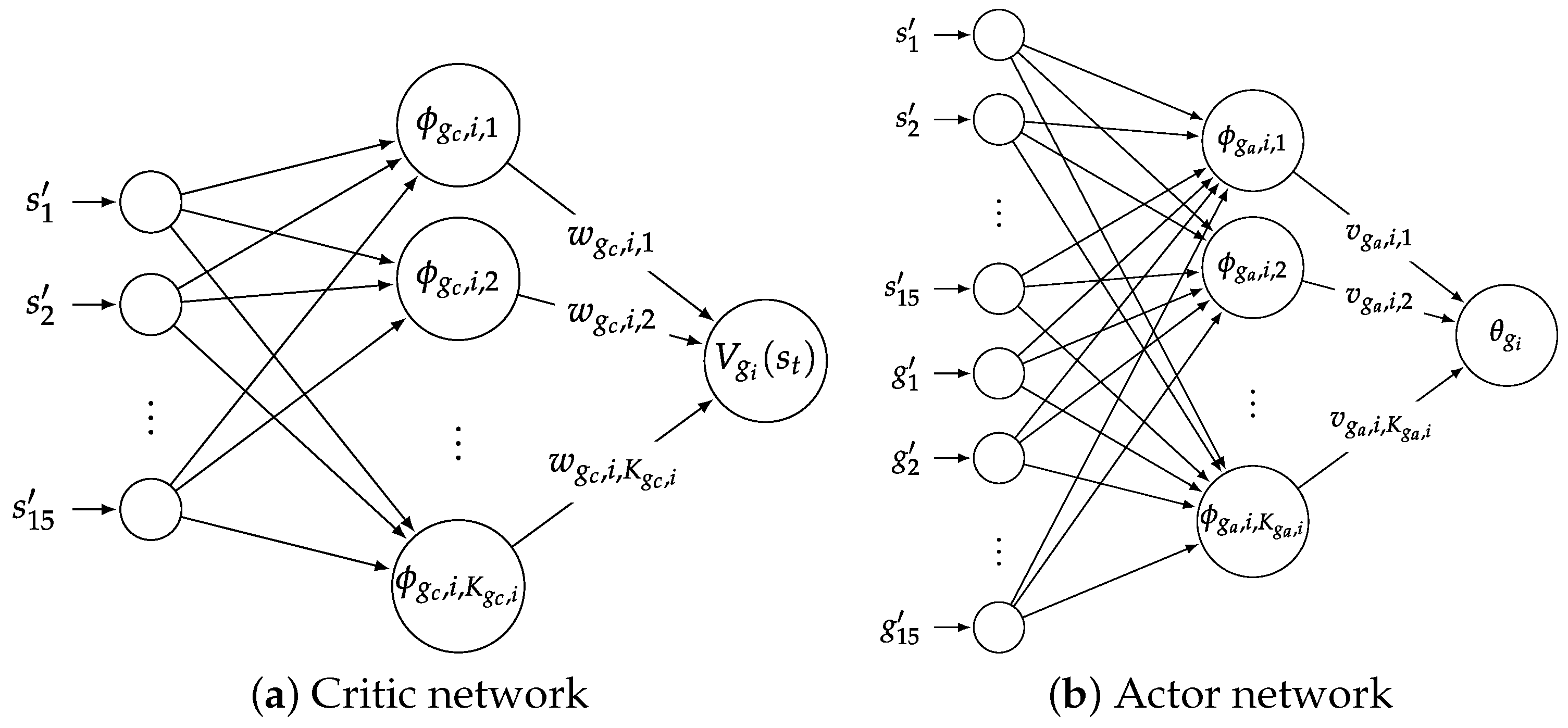
We use the actor-critic RL algorithm to synthesize the self-tuning two-degree-of-freedom PI control system. We introduced RBF networks to both the actor and critic independently. The critic networks are trained to approximate the value function of the states, whereas the actor networks learn to determine internal policy parameters to maximize the return. We propose to introduce the spatial coefficients $\eta$ for spatial augmentation of the error and the reward to help proceed with appropriate learning under the existence of input coupling. The performance of the proposed control system is evaluated through numerical simulations under several likely scenarios in the operation of industrial processes. The results demonstrate the superiority of the proposed control system over the fixed-gain PI controller.

Although we concentrate on the development of the self-tuning two-DOF PI controller for the film production process in this study, the idea of the spatial augmentation of the error and the reward can be applied to other plants that also suffer from input coupling.

Table 1. Number of academic documents related to PID control for industrial processes that were published in the past twenty years and indexed in the academic document portals.

Five-Year Period	2001–2005	2006–2010	2011–2016	2016–Present
Portal A	212	381	584	610
Portal B	188	331	348	426

summarizes the number of documents published in the past twenty years that state the development of PID control systems for industrial processes.

The figures in the table clearly shows that there exists a consistent and strong demand for the use of PID controllers for process control problems, and their increasing trend predicts that PID controllers will continue to be used in various control problems in the future. The enhancement of PID control for process control problems developed in this article will continue to remain valuable in this light.

2. Description of the Target Process

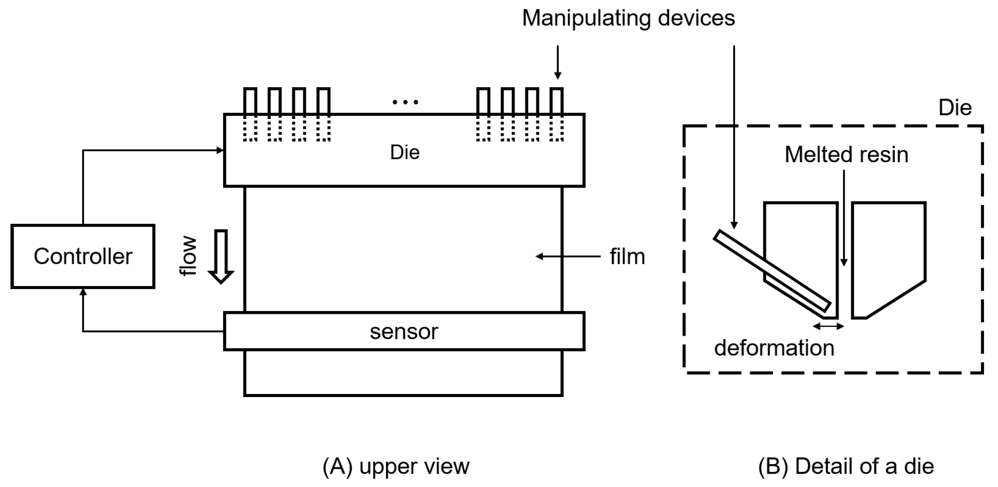
We aim to synthesize a control system for a thin plastic film fabrication process. The objective of the control system is to fabricate a plastic film that has a spatially uniform designated thickness. Figure 1 shows the control related schematics of the film fabrication machine. The thickness of the fabricated film is controlled by a die aligned orthogonal to the flow of melted resin. The width of the die is 63 mm. Fifteen die-manipulating devices are aligned linearly on a die with a 4 mm interval, as shown in Figure 2. We can measure the thickness of a film with a spatial resolution of 1 mm, as shown in Figure 2; however, we cannot monitor the cross-sectional shape of the die.

The displacement of each device can be controlled independently. We performed a step response experiment with a single manipulating device and measured its response. The transfer function of a manipulating device from its input $u\left(t\right)$ to the displacement $y\left(t\right)$ is accordingly identified to be:

$$\begin{array}{c}\hfill {\displaystyle P\left(s\right)=\frac{Y\left(s\right)}{U\left(s\right)}=\frac{0.006}{120s+1}exp(-95s),}\end{array}$$

(1)

where $u\left(t\right)$ takes a value within the interval $[0,100]$ and $y\left(t\right)$ is measured in units of millimeters (mm). We hereafter assume that all manipulating devices are characterized by the transfer function (1) in their nominal operating condition.

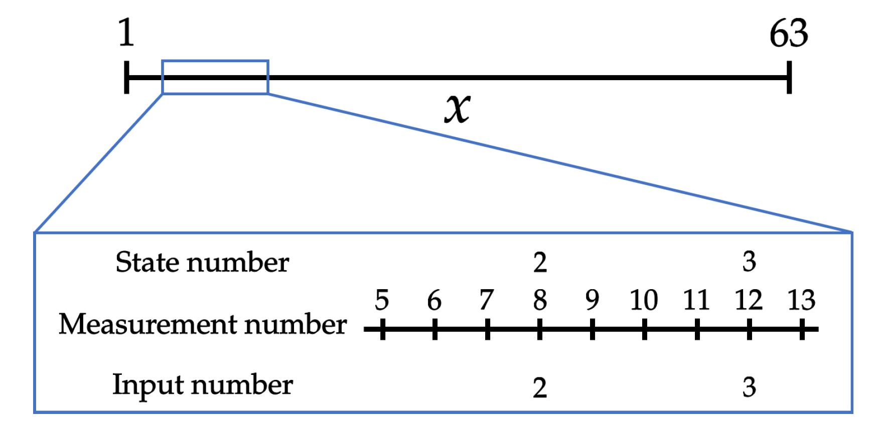
The actual shape of the cross-section of a die is determined by the displacements of the manipulating devices. The displacement of a die where a particular manipulating device is located is determined not only by the displacement of the corresponding device, but also by the displacements of other manipulating devices located nearby. 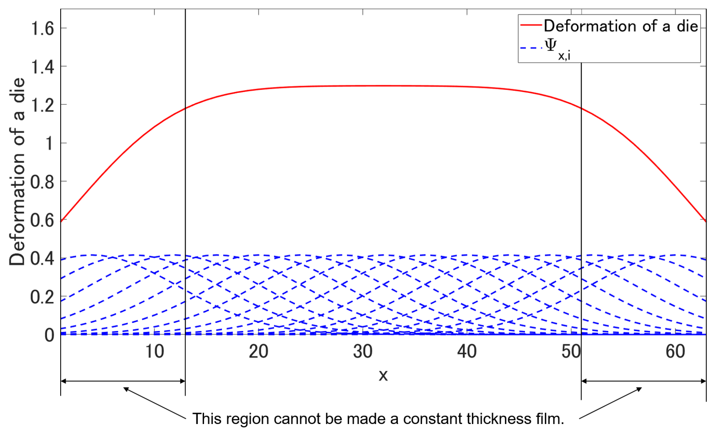Let $x\in (0,63]$ be the position of a film, and let $c_i(i=1,2,\cdots ,15)$ be the location of the i-th manipulating device, as shown in Figure 2. We model the spatial coupling of the manipulating devices with the function ${\mathsf{\Psi }}_{x,i}(i=1,2,\cdots ,N)$ given by:

$$\begin{array}{c}\hfill {\mathsf{\Psi }}_{x,i}=0.415exp(-{\left(0.085d_{x,i}\right)}^2),\end{array}$$

(2)

where $d_{x,i}=\parallel x-c_i\parallel$ is the distance between the position x and the i-th manipulating device. The blue broken lines in Figure 3 show ${\mathsf{\Psi }}_{x,i}$ for all i. The displacement of a die at position x can be calculated as:

$$\begin{array}{c}\hfill f\left(x\left(t\right)\right)=\sum _{i=1}^N{\mathsf{\Psi }}_{x,i}{y}_i\left(t\right),\end{array}$$

(3)

where $y_i\left(t\right)$ represents the displacement of the i-th manipulating device at time t and $N=15$ is the number of die-manipulating devices installed in the process.

We calculated the steady-state deformation of the die by letting $u_i\left(t\right)=100(\forall i)$ and kept them until all the outputs $y_i\left(t\right)$ converged. The red solid plot in Figure 3 shows the final form of the deformation of a die as calculated using Equation (3). This figure shows that the deformation of the left and right edges of the die will not reach its maximum. Therefore, in some cases, the thickness of the fabricated film cannot be made constant if the reference thickness is too small. We define the control objective accordingly to regulate the thickness of the fabricated film corresponding to the region $13<x<51$ of the die to be equal to its reference, denoted hereafter as $s_{\mathrm{ref}}$.

3. Control System Synthesis for the Film Fabrication Process

3.1. Structure of the Proposed Control System

Herein, we propose a two-degree-of-freedom (two-DOF) PI control system for a thin film fabrication process whose gains and feed-forward terms are tuned online by an actor-critic-type RL algorithm. We first define the signals used by the controller. Because we implemented the proposed control system with a digital computer, we hereafter use a discrete time description for the signals included in the system. However, the dynamics of manipulating devices are still described by a continuous-time s-domain transfer function because the manipulating devices should be considered continuous-time plants.

Since each manipulating device is known to suffer a nominal lag of $L=95$ s, we applied the Smith predictor structure for each manipulating device, as shown in Figure 4, wherein $a_{ff},a_P$, and $a_I$ represent the feed-forward input, the proportional gain vector, and the integral gain vector, respectively. $\eta$ denotes a spatial augmentation coefficient for the compensation of input coupling, as will be detailed later. Let $P_M\left(s\right)$ be the transfer function defined as:

$$\begin{array}{c}\hfill P_M\left(s\right)=\frac{0.006}{120s+1}.\end{array}$$

(4)

Let $T_s=3$ denote the sampling interval of the control system. Hereafter, we use the sampling number index m to describe the current signal values at $t=m{T}_s$. Let $s_M\left[m\right]$ be the response of $P_M\left(s\right)$ to the input signal sequence $u\left[m\right]$. The signal $s\left[m\right]$ to be fed to both the PI controller and the RL block is defined as:

$$\begin{array}{c}\hfill s\left[m\right]=s_M\left[m\right]+s_P\left[m\right]-s_M[m-L_D],\end{array}$$

(5)

where $L_D=\lfloor L/T_s\rfloor$ denotes the sampling number that approximates the nominal lag L. We define the signal $s_P\left[m\right]$ as the measured thickness of a film corresponding to a specific manipulating device. Because $L_D\times T_s\ne L$ and we cannot measure the individual displacement of a manipulating device, we note that the feedback control structure shown in Figure 4 is not a perfect implementation of the Smith predictor.

3.2. Two-DOF PI Controller Tuned by RL Algorithm

We implemented the feedback control structure shown in Figure 4 for the control of each manipulating device. Hereafter, we denote the signal $s\left[m\right]$ for the i-th manipulating device as $s_i\left[m\right](i=1,2,\cdots ,N)$. Let:

$$\begin{array}{cc}\hfill {\epsilon }_i\left[m\right]& =\frac{s_i\left[m\right]-s_{\mathrm{ref}}}{{\epsilon }_{\max }}\hfill \end{array}$$

(6)

be the normalized tracking error variable for the i-th manipulating device. We accordingly define its summation as:

$$\begin{array}{cc}\hfill {\epsilon }_i^{\sum }\left[m\right]& ={\epsilon }_i^{\sum }[m-1]+{\epsilon }_i[m-1]\hfill \end{array}$$

(7)

The control law to be synthesized for the i-th manipulating device is described as:

$$\begin{array}{c}\hfill u_i=a_{ff,i}+{\mathit{a}}_{P,i}^T{\overline{\mathit{\epsilon }}}_i+{\mathit{a}}_{I,i}^T{\overline{\mathit{\epsilon }}}_i^{\sum },\end{array}$$

(8)

where $a_{ff,i}$ represents the feed-forward control input, and the remaining terms constitute a PI controller for the i-th manipulating device. The error ${\overline{\mathit{\epsilon }}}_i$ and its summation ${\overline{\mathit{\epsilon }}}_i^{\sum }$ that appear in (8) are the vectors defined as:

$$\begin{array}{cc}\hfill {\overline{\mathit{\epsilon }}}_i& ={[{\overline{\epsilon }}_{i,1},\cdots ,{\overline{\epsilon }}_{i,N}]}^T\hfill \end{array}$$

(9)

and:

$$\begin{array}{cc}\hfill {\overline{\mathit{\epsilon }}}_i^{\sum }& ={[{\overline{\epsilon }}_{i,1}^{\sum },\cdots ,{\overline{\epsilon }}_{i,N}^{\sum }]}^T,\hfill \end{array}$$

(10)

respectively. ${\overline{\epsilon }}_{i,j}$ is a spatially augmented error defined as:

$$\begin{array}{cc}\hfill {\overline{\epsilon }}_{i,j}& ={\eta }_{i,j}{\epsilon }_j,\hfill \end{array}$$

(11)

where ${\eta }_{i,j}$ is a coefficient that is defined to consider ${\epsilon }_j\left[m\right](j=1,2,\cdots ,N)$ in (6) for the control of the i-th manipulating device. We introduce the spatial error augmentation to compensate for the mechanical coupling of the manipulating devices, which would worsen the film thickness accuracy. This setup yielded the PI gains ${\mathit{a}}_{P,i}$ and ${\mathit{a}}_{I,i}$ to be vectors in ${\mathit{R}}^N$.

4. Actor-Critic RL to Self-Tune Controller Constants

4.1. Parameterized Policy and Policy Gradient RL for Self-Tuning Controller Parameters

The tuning of controller parameters of a process is considered to be highly empirical and require experienced operators to run the process stably under various uncertainties. We regard the control law defined in (8) to be the deterministic policy and employ RL for the self-tuning of the parameters in this policy based on the observed control performance. The parameters to be tuned are $a_{ff,i}$, ${\mathit{a}}_{P,i}$, ${\mathit{a}}_{I,i}$, and ${\eta }_{i,j}$. We include tunable parameters $\mathsf{\Theta }$ in these quantities and update their values to maximize the expected return $\mathbb{E}\left\{R_t\right|\mathsf{\Theta }\}$. The learning scheme is classified as the policy-gradient-type actor-critic algorithm proposed by Kimura and Kobayashi [20].

We define the control actions for the i-th manipulating device included in the deterministic policy (8) as:

$$\begin{array}{cc}\hfill a_{ff,i}& {\displaystyle =a_{ff,i}+\sum _{j=1}^N\frac{a_{ff,\max }}{1+exp(-{\theta }_{ff,i,j})}\frac{{\overline{\epsilon }}_{i,j}}{G_{a_{ff}}}(j=1,2,\cdots ,N)}\hfill \end{array}$$

(12)

$$\begin{array}{cc}\hfill a_{*,i,j}& {\displaystyle =\frac{a_{*,\max }}{1+exp(-{\theta }_{*,i,j})}(*\in \{P,I\})}\hfill \end{array}$$

(13)

and:

$$\begin{array}{c}\hfill \begin{array}{cc}\hfill {\eta }_{i,j}& =exp(-g_i·\parallel c_i-c_j{\parallel }^2)\hfill \\ \hfill g_i& =\frac{g_{\max }}{1+exp(-{\theta }_{g_i})}-\frac{1}{2}{g}_{\max }+g_i\left(0\right),\hfill \end{array}\end{array}$$

(14)

where ${\theta }_{ff,i,j}$, ${\theta }_{P,i,j}$, ${\theta }_{I,i,j}$, and ${\theta }_{g_i}$ are the internal policy parameters for the feedforward, proportional, and integral control actions and the spatial coefficient ${\eta }_{i,j}$, respectively. $G_{a_{ff}}$, $a_{ff,\max }$, $a_{P,\max }$, $a_{I,\max }$, and $g_{\max }$ are suitably chosen constants. As each manipulating device has a long time constant and suffers a large delay, the feedforward control term $a_{ff,i}$ is used to facilitate a faster response.

4.2. RBF Networks for Actor-Critic RL

4.2.1. Critic Network

In this study, continuous changes in the states and actions of the RL algorithm must be assumed. Therefore, we used RBF networks that map the observed signals to quantities used in learning and control.

The critic network approximates the value function $V\left(s\right[m\left]\right)$ for the film thickness measurement $s\left[m\right]={[s_1\left[m\right],s_2\left[m\right],\cdots ,s_N\left[m\right]]}^T$. We calculated the normalized version of $s\left[m\right]$ denoted by ${\mathit{s}}^{\prime }\left[m\right]={[s_1^{\prime }\left[m\right],\cdots ,s_{15}^{\prime }\left[m\right]]}^T$. $s_i^{\prime }$ linearly maps the interval $[0.5s_{\mathrm{ref}},1.5s_{\mathrm{ref}}]$ of $s_i$ to $[0,1]$. Figure 5 shows the structure of the critic network.

The k-th hidden layer node ${\varphi }_{i,k}(k=1,2,\cdots ,K_i;K_i\le K_{\max })$ is described as:

$$\begin{array}{c}\hfill {\varphi }_{i,k}=exp\left(-\frac{{(s^{\prime }-{\mu }_{i,k})}^T(s^{\prime }-{\mu }_{i,k})}{\rho {\sigma }_{i,k}^2}\right)(k=1,2,\cdots ,K_i),\end{array}$$

(15)

where ${\mu }_{i,k}={[{\mu }_{i,1,k},\cdots ,{\mu }_{i,N,k}]}^T,{\sigma }_{i,k}$ defines the center and the standard deviation of the RBF function, respectively. The parameter $\rho$ controls the tailedness of the RBFs. The number of hidden layer nodes $K_i$ will be increased dynamically within the predefined maximal number $K_{\max }$ to improve the precision of the approximation for a wide range of state spaces. The value function $V_i\left(s\left[m\right]\right)$ is defined as:

$$\begin{array}{c}\hfill V_i\left(s\left[m\right]\right)=\sum _k{w}_{i,k}{\varphi }_{i,k},\end{array}$$

(16)

where $w_{i,k}$ is a weight. The parameters of the critic network, $w_{i,k}$, ${\mu }_{i,k}$, and ${\sigma }_{i,k}$, are updated so as to make the index:

$$\begin{array}{c}\hfill J_i=\frac{1}{2}{\delta }_i^2\end{array}$$

(17)

small. ${\delta }_i$ is a temporal difference (TD) error defined as:

$$\begin{array}{cc}\hfill {\delta }_i& =r_i+\gamma V_i\left(s[m+1]\right)-V_i\left(s\left[m\right]\right),\hfill \end{array}$$

(18)

and $r_i$ is an instantaneous reward calculated as:

$$\begin{array}{cc}\hfill S{S}_i& =\mathsf{\Delta }{\epsilon }_i+B{\epsilon }_i\hfill \\ \hfill r_i& {\displaystyle =\sum _j{\eta }_{i,j}S{S}_j^2\left(\right|r_i|\le 1),}\hfill \end{array}$$

(19)

where $\mathsf{\Delta }{\epsilon }_i\stackrel{▵}{=}({\epsilon }_i\left[m\right]-{\epsilon }_i[m-1])/T_s$ is the backward difference of the sequence ${\epsilon }_i\left[m\right]$ and $S{S}_i$ defines a stable hypersurface of the error such that $S{S}_i\to 0$ indicates ${\epsilon }_i\to 0$. The gradient of the hypersurface B must be determined appropriately for this purpose. The update laws of the critic network parameters follow the policy-gradient algorithm, specifically defined as:

$$\begin{array}{cc}\hfill w_{i,k}& =w_{i,k}+{\alpha }_w{\delta }_i{D}_{i,k}\hfill \end{array}$$

(20)

$$\begin{array}{cc}\hfill {\mu }_{i,k}& ={\mu }_{i,k}+{\alpha }_{\mu }{\delta }_i{w}_{i,k}{D}_{i,k}\frac{2(s^{\prime }-{\mu }_{i,k})}{\rho {\sigma }_{i,k}^2}\hfill \end{array}$$

(21)

$$\begin{array}{cc}\hfill {\sigma }_{i,k}& ={\sigma }_{i,k}+{\alpha }_{\sigma }{\delta }_i{w}_{i,k}{D}_{i,k}\frac{2{(s^{\prime }-{\mu }_{i,k})}^T(s^{\prime }-{\mu }_{i,k})}{\rho {\sigma }_{i,m}^3}\hfill \end{array}$$

(22)

where ${\alpha }_w$, ${\alpha }_{\mu }$, and ${\alpha }_{\sigma }$ define the learning rates for w, $\mu$, and $\sigma$, respectively, and $D_{i,k}$ is an eligibility trace defined as:

$$\begin{array}{cc}\hfill D_{i,k}& =\gamma \lambda D_{i,k}+{\varphi }_{i,k}.\hfill \end{array}$$

4.2.2. Actor Network

The actor networks are configured to approximate the internal policy parameters included in (12) and (13). Figure 6 shows the structure for the feedforward control action parameters ${\theta }_{ff,i,j}$ and the PI control action parameters ${\theta }_{P,i,j}$ and ${\theta }_{I,i,j}$. The feedforward actor network is designed to receive the normalized state ${\mathit{s}}^{\prime }$ and the normalized policy parameter $a_{ff}^{\prime }={[a_{ff,1}^{\prime },\cdots ,a_{ff,N}^{\prime }]}^T$ as its input, and the actor networks use the normalized state ${\mathit{s}}^{\prime }$ and the normalized control gains $a_{*,i}={[a_{*,i,1}^{\prime },\cdots ,a_{*,i,15}^{\prime }]}^T(*\in \{P,I\})$ as their inputs.

The k-th hidden layer node ${\varphi }_{**,i,j}^{\left(k\right)}$ for the i-th actor networks is defined by an RBF:

$$\begin{array}{cc}\hfill {\varphi }_{**,i,j}^{\left(k\right)}& =exp\left(-\frac{{(x_{**,i}-{\mu }_{q,i,j}^{\left(k\right)})}^{\mathrm{T}}(x_{**,i}-{\mu }_{**,i,j}^{\left(k\right)})}{\rho {\left({\sigma }_{**,i,j}^{\left(k\right)}\right)}^2}\right),\hfill \end{array}$$

(23)

where its argument ${\mathit{x}}_{**,i}$ is defined as:

$$\begin{array}{cc}\hfill x_{ff,i}& ={[s_1^{\prime },\cdots ,s_{15}^{\prime },a_{ff,1}^{\prime },\cdots ,a_{ff,15}^{\prime }]}^T\hfill \end{array}$$

for the feedforward network and:

$$\begin{array}{cc}\hfill x_{*,i}& ={[s_1^{\prime },\cdots ,s_{15}^{\prime },a_{*,i,1}^{\prime },\cdots ,a_{*,i,15}^{\prime }]}^T(*\in \{P,I\})\hfill \end{array}$$

for the PI controller networks.

Both the feedforward and the PI actor networks aim to tune ${\theta }_{*,i,j}(*\in \{ff,P,I\})$ using their network parameters v, $\mu$, and $\sigma$. We applied the policy-gradient method to the learning of the actor networks. The update laws of the RBF parameters were synthesized as:

$$\begin{array}{c}\hfill \begin{array}{c}\hfill v_{**,i,j}^{\left(k\right)}\leftarrow v_{**,i,j}^{\left(k\right)}+{\alpha }_{**}{\delta }_i{D}_{v_{**,i,j}^{\left(k\right)}}\\ \hfill {\mu }_{**,i,j}^{\left(k\right)}\leftarrow {\mu }_{**,i,j}^{\left(k\right)}+{\alpha }_{a\mu }{\delta }_i{D}_{{\mu }_{**,i,j}^{\left(k\right)}}\\ \hfill {\sigma }_{**,i,j}^{\left(k\right)}\leftarrow {\sigma }_{**,i,j}^{\left(k\right)}+{\alpha }_{a\sigma }{\delta }_i{D}_{{\sigma }_{**,i,j}^{\left(k\right)}}\end{array}\end{array}$$

(24)

to maximize the expected return $\mathbb{E}\left\{R_t\right\}$, where $\ast \ast$ represents either $ff$, P, or I. $D_v$, $D_{\mu }$, and $D_{\sigma }$ are the eligibility traces characterized as:

$$\begin{array}{cc}\hfill D_{v_{**,i,j}^{\left(k\right)}}& =\gamma \lambda D_{v_{**,i,j}^{\left(k\right)}}+\frac{\partial u_i}{\partial v_{**,i,j}^{\left(k\right)}}\hfill \\ \hfill D_{{\mu }_{**,i,j}^{\left(k\right)}}& =\gamma \lambda D_{{\mu }_{**,i,j}^{\left(k\right)}}+\frac{\partial u_i}{\partial {\mu }_{**,i,j}^{\left(k\right)}}\hfill \\ \hfill D_{{\sigma }_{**,i,j}^{\left(k\right)}}& =\gamma \lambda D_{{\sigma }_{**,i,j}^{\left(k\right)}}+\frac{\partial u_i}{\partial {\sigma }_{**,i,j}^{\left(k\right)}},\hfill \end{array}$$

(25)

where ${\alpha }_{\ast \ast }$, ${\alpha }_{a\mu }$, and ${\alpha }_{a\sigma }$ are the corresponding learning rates.

4.3. Learning Spatial Coupling Coefficient ${\eta }_{i,j}$

We introduced the spatial coupling coefficient ${\eta }_{i,j}$ to compensate for the mechanical coupling of the die manipulating devices. As their coupling form cannot be known prior to operation and may vary within consecutive runs, we tried to tune the parameter $g_i$ included in ${\eta }_{i,j}$ to improve the control performance.

We also applied the actor-critic structure with the RBF network shown in Figure 7 to self-tune $g_i$. Each node in the hidden layer RBF is fully connected to the inputs of the networks. The critic function attempts to learn the value function $V_{g_i}$ for ${\eta }_{i,j}$, whereas the actor network tunes the internal policy parameter ${\theta }_{g_i}$ in (14) to minimize the performance index defined by $J_{g_i}^a={\epsilon }_i^2/2$.

Similar to the actor-critic networks for the two-DOF PI self-tuning control system, the learning targets $V_{g_i}$ (for critic) and ${\theta }_{g_i}$ (for actor) are the functions of the network parameters. The learning rules to be formulated should target the network parameters, namely the center and variance of the RBFs in hidden layer nodes and weights to synthesize the outputs of the networks.

The critic network parameters were updated to minimize the squared form $J_{g_i}^c={\delta }_{g_i}^2/2$ of a TD-error ${\delta }_{g_i}$ defined as:

$$\begin{array}{cc}\hfill {\delta }_{g_i}& =r_{g_i}+\gamma V_{g_i}\left(s[m+1]\right)-V\left(s\left[m\right]\right),\hfill \end{array}$$

where the instantaneous reward $r_{g_i}$ is defined as:

$$\begin{array}{cc}\hfill r_{g_i}& =-\sum _j{\eta }_{i,j}{\epsilon }_j^2(\mid r_{g_i}\mid \le 1).\hfill \end{array}$$

The parameters of the actor network are updated to the negative gradient direction of the performance index $J_{g_i}^a={\epsilon }_i^2/2$ to make $J_{g_i}^a$ small. Because the resulting update laws for the actor-critic network of the internal policy parameter $g_i$ will appear quite similar to those dictated to the actor-critic RL of a two-DOF PI control system, they are omitted to avoid repetition. We finally summarize the calculation flow of our proposed control system in Algorithm 1.

Algorithm 1 Calculation flow of the proposed two-DOF self-tuning PI control system.

5. Performance Evaluation through Numerical Simulations

We performed numerical simulations under several likely scenarios to demonstrate the performance of the proposed control system. As a representative conventional process control technique, we synthesized a static PI controller using the Ziegler–Nichols (Z.N.) ultimate gain method. We applied the same set of gains to all N manipulating devices and configured the spatial coupling coefficient ${\eta }_{i,j}$ as:

$$\begin{array}{c}\hfill {\eta }_{i,j}=\left\{\begin{array}{c}1(i=j)\hfill \\ 0(i\ne j)\hfill \end{array}\right.\end{array}$$

(26)

to evaluate how much ${\eta }_{i,j}$ would be effective in compensating for the intrinsic mechanical coupling caused by manipulating devices other than the i-th one.

To quantify the control performance, we calculated the spatial root mean squared error (sRMSE), defined as:

$$\begin{array}{cc}\hfill \mathrm{sRMSE}\left[m\right]& {\displaystyle =\sqrt{\frac{1}{37}\sum _{x=14}^{50}{(s_{\mathrm{ref}}-thickness\left(x\right))}^2},}\hfill \end{array}$$

(27)

where $thickness\left(x\right)$ is the film thickness measured at the labeled position x in Figure 2.

Table 2. Parameters used to formulate actor and critic networks for self-tuning the two-DOF PI control system.

Parameter	Value
Critic network parameters
Learning rate of weights ${\alpha }_w$ in (20)	$1.0\times {10}^{-5}$
Learning rate of RBF center ${\alpha }_{\mu }$ in (21)	$1.0\times {10}^{-6}$
Learning rate of variance ${\alpha }_{\sigma }$ in (22)	$1.0\times {10}^{-6}$
Discount rate $\gamma$	0.99
Trace attenuation parameter $\lambda$	0.99
Actor network parameters
${\alpha }_{ff}$ for $a_{ff}$	$5.0\times {10}^{-3}$
${\alpha }_P$ for ${\mathit{a}}_P$	$1.0\times {10}^{-6}$
${\alpha }_I$ for ${\mathit{a}}_I$	$1.0\times {10}^{-6}$
${\alpha }_{a\mu }$ for actor RBF	$1.0\times {10}^{-6}$
${\alpha }_{a\sigma }$ for actor RBF	$1.0\times {10}^{-6}$
$a_{ff,\max }$	100
$a_{P,\max }$	350
$a_{I,\max }$	50
$G_{a_{ff}}$ for $a_{ff}$ in (13)	8

and

Table 3. Parameters related to ${\eta }_{i,j}$ and rewards.

Parameter	Value
Parameters for spatial coupling coefficient ${\eta }_{i,j}$
${\alpha }_{gc}$ for critic RBF network	$1.0\times {10}^{-3}$
${\alpha }_{g_c\mu }$ for critic RBF unit	$1.0\times {10}^{-4}$
${\alpha }_{g_c\sigma }$ for critic RBF unit	$1.0\times {10}^{-4}$
${\alpha }_{g_a}$ for actor RBF network	$2.0\times {10}^{-2}$
${\alpha }_{g_a\mu }$ for actor RBF unit	$1.0\times {10}^{-4}$
${\alpha }_{g_a\sigma }$ for actor RBF unit	$1.0\times {10}^{-4}$
$g_i\left(0\right)$ (initial value of $g_i$)	0.06
$g_{\max }$	2
Other parameters
$\rho$ (controls tailedness of RBF)	$2.5$
Gradient of hypersurface B	0.2

respectively list the actor and critic network parameters used in the simulation.

The sampling interval was set as 3 s in all simulation scenarios. We added random noise to the calculated thickness to simulate measurement noise. The noise was generated within a $\pm 0.5\%$ range of the reference thickness of a film.

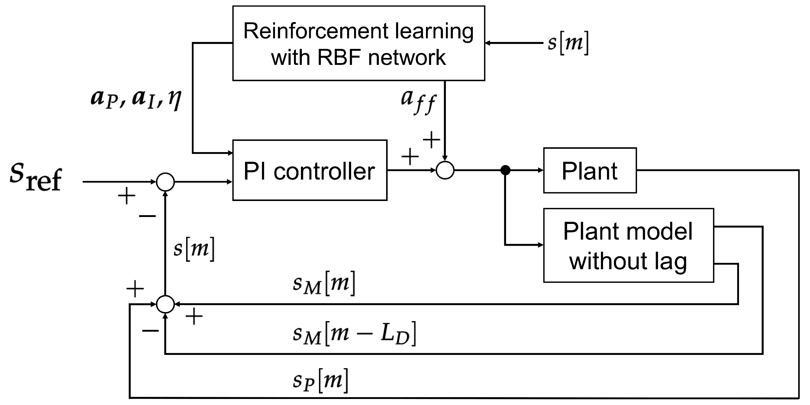
In the following scenarios, we applied three different controllers: (1) the proposed self-tuning two-DOF PI controller, (2) the proposed self-tuning two-DOF PI controller, but with ${\eta }_{i,j}$ defined using (26), and (3) the static gain PI controller whose gains were determined using the Z.N. ultimate gain method. We uniformly applied the feedback control structure shown in Figure 4 to all three controller setups in all scenarios. We only disabled the RL calculations when we tried to obtain control results with static PI controllers. For the self-tuning control simulations, we repeated the simulation with an identical initial thickness distribution for 40 episodes. The results corresponding to the 41st episode are shown below. We note that the number of RBF nodes in the hidden layer of the actor and critic networks were set to zero initially and increased automatically. We applied the algorithm for the automatic addition of RBF nodes proposed by Kamaya et al. [21] whilst making necessary changes to adapt to our MIMO control problem.

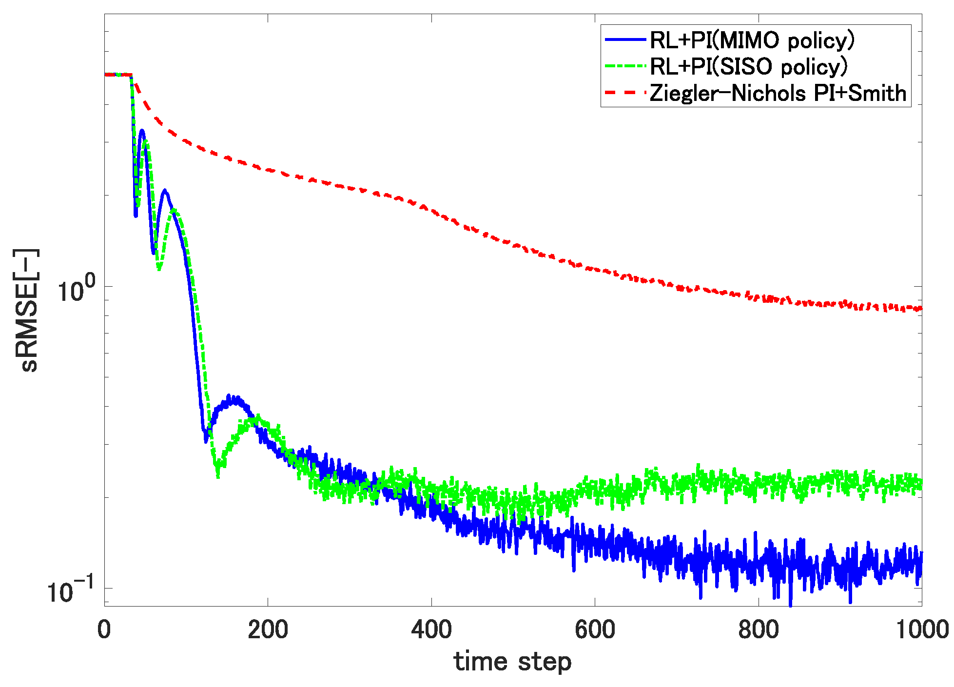
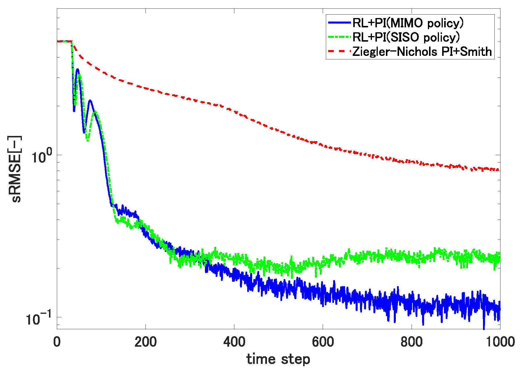
5.1. sRMSE Trajectories for a Fixed Reference Thickness

We first set the reference thickness to 70 and observed the transient changes in the sRMSE metrics. Figure 8 shows the result.

The plots indicate that the proposed self-tuning controllers not only yielded much faster convergence, but also achieved significantly smaller sRMSE values than the conventional static PI controller. The figure also shows that incorporating the spatial coupling coefficient ${\eta }_{i,j}$ defined using (14) and the associated learning scheme resulted in a smaller sRMSE than that achieved with the decoupled self-tuning controller corresponding to ${\eta }_{i,j}$ defined using (26).

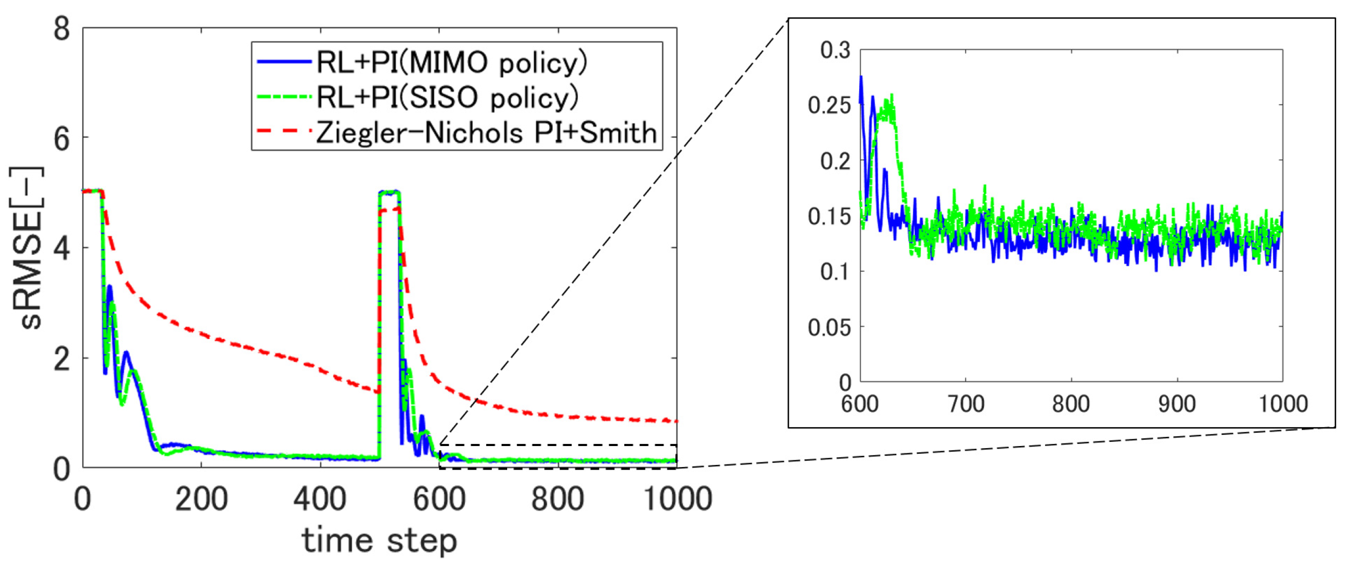
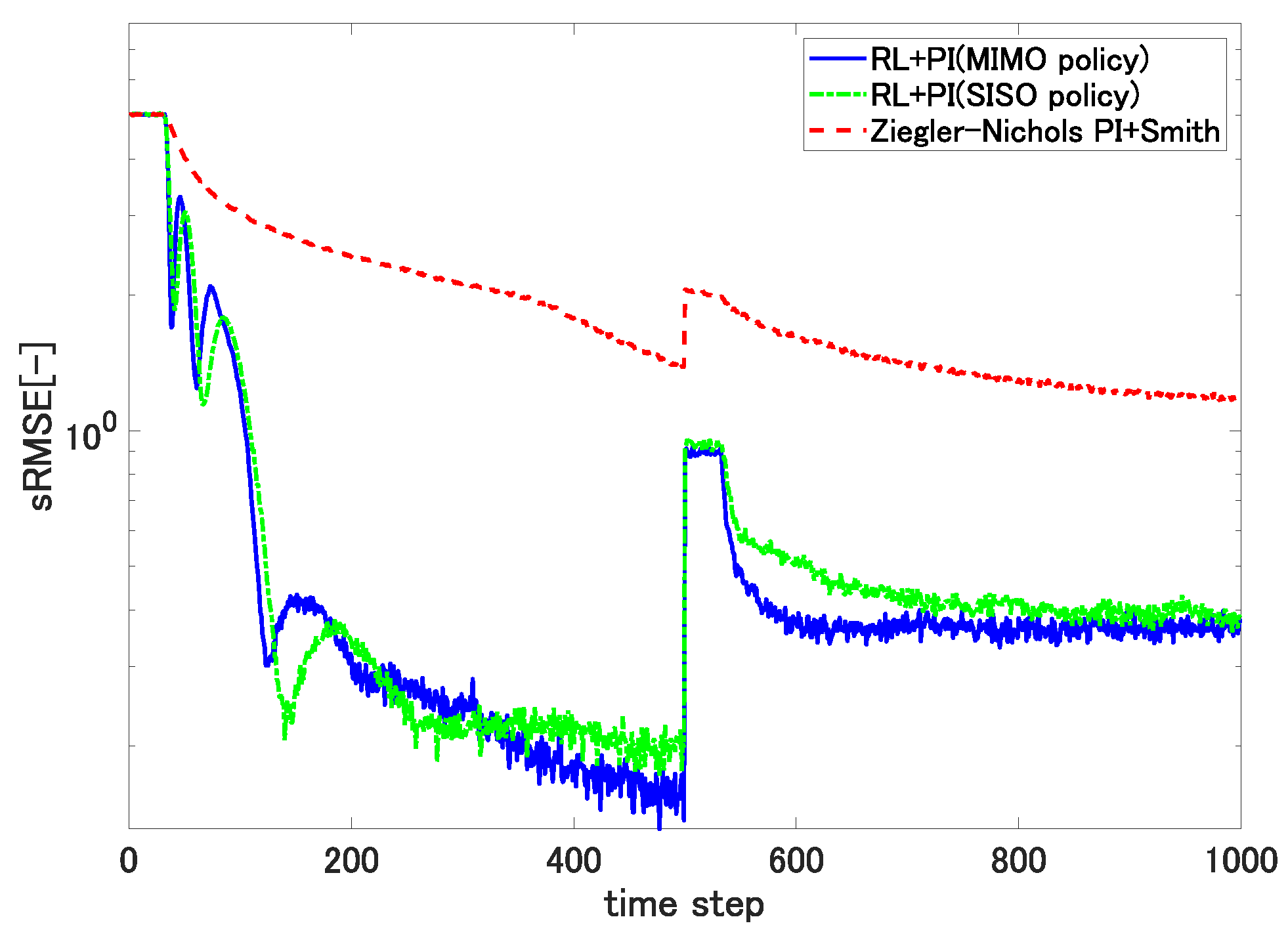
5.2. Response to Changes in Reference Film Thickness

Although the real film production process does not change the reference thickness within a single production batch, we changed the reference thickness from 70 to 65 at the 500th sampling step in the 41st episode to observe the response after completing 40 episodes with a constant reference thickness of 70. Figure 9 shows the result.

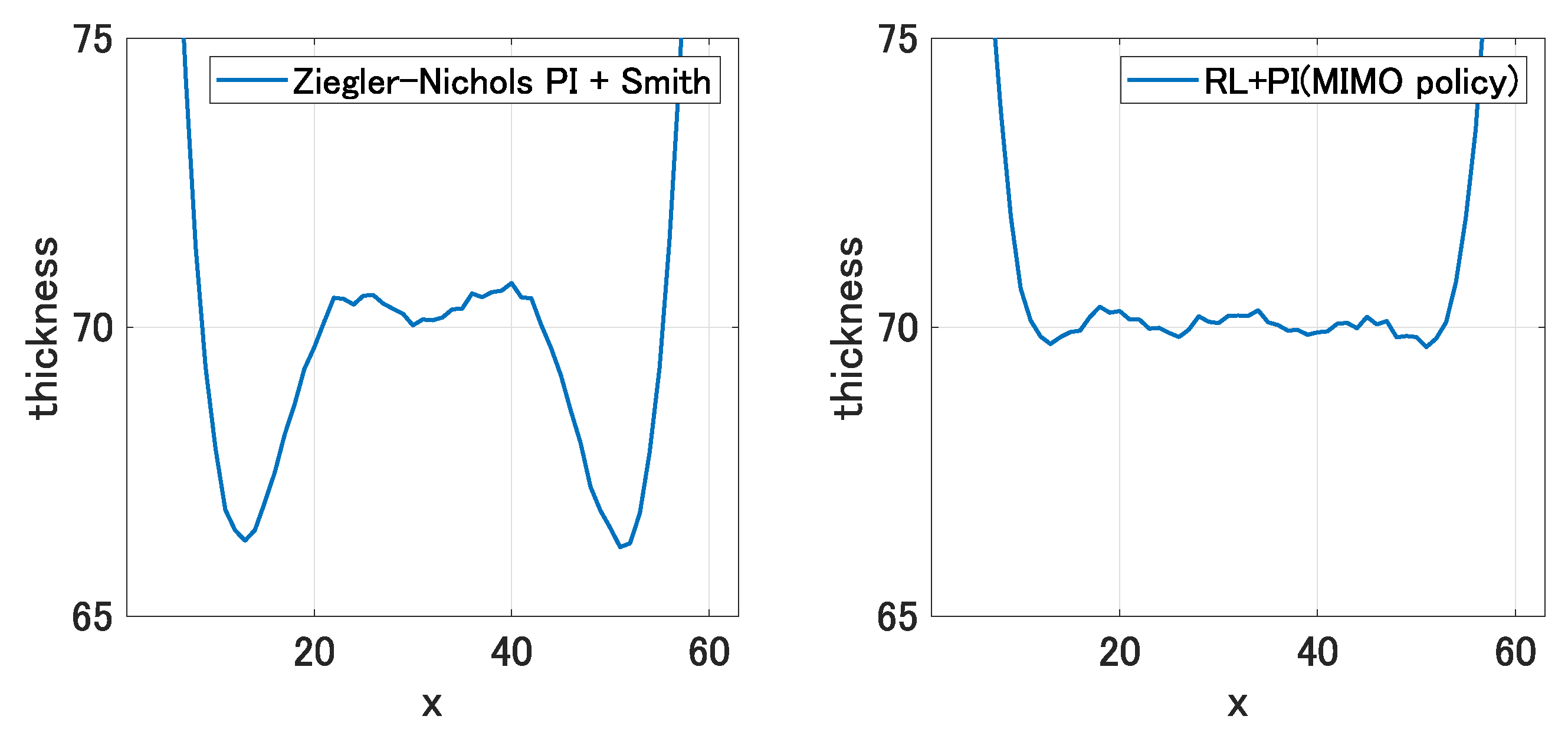
The proposed self-tuning controllers again exhibited much smaller sRMSE metrics than the static PI controller. ${\eta }_{i,j}$ defined using (14) with the associated RL produced better accuracy than the SISO self-tuning controller, as was also observed in the previous scenario. Although the self-tuning controllers temporarily exhibited larger sRMSEs than the static PI controller after the reference thickness was altered, this was an incidental issue as evidenced by the film thickness distributions corresponding to the Z.N. 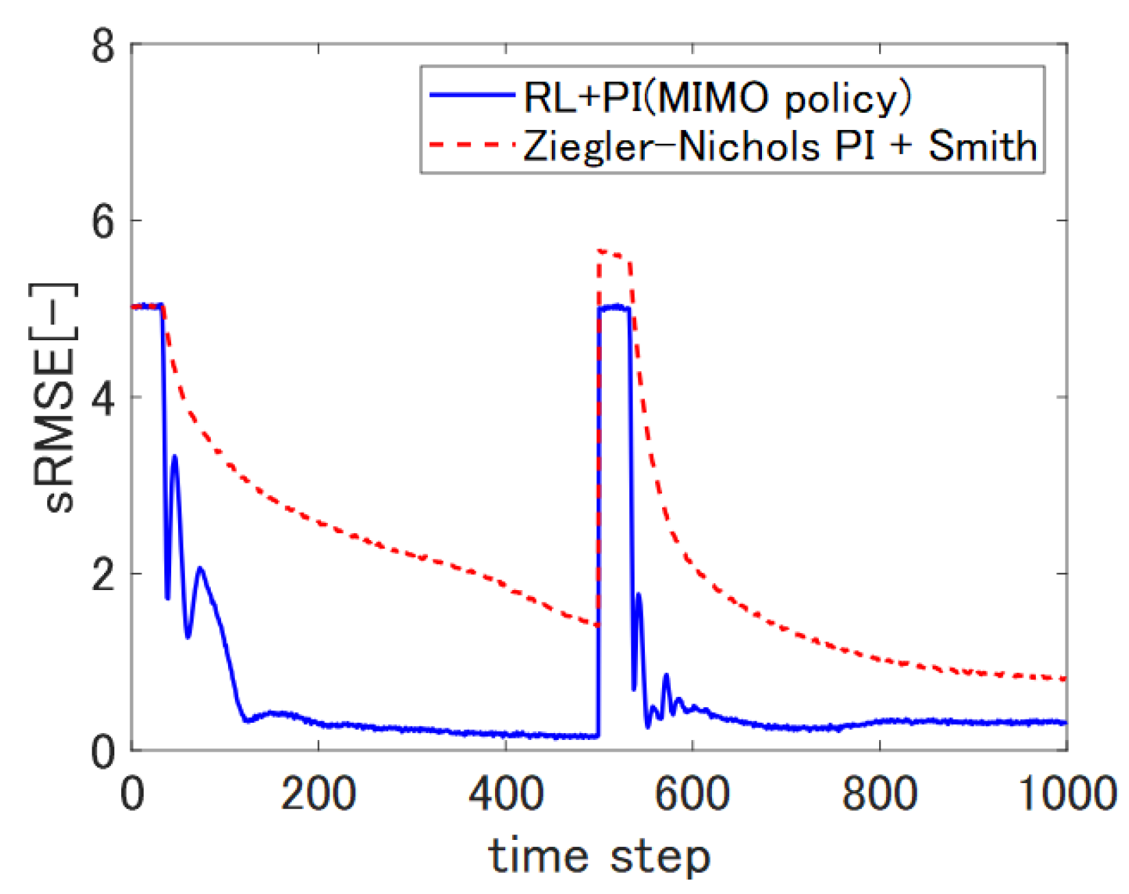PI and the proposed controller in Figure 10. Since the film corresponding to the Z.N. PI controller has portions apparently thinner than 70 and closer to the new reference of 65, it temporarily exhibited a smaller sRMSE metric than film generated by the proposed controller whose thickness was uniformly close to 70. Our inference was further justified by the additional simulation in which the new reference was set to be 75, which is larger than 70. The result is shown in Figure 11.

The recovery of the sRMSE metric after the change of the reference thickness corresponding to our proposed controller as shown in Figure 9 and Figure 11 revealed that the proposed controller exhibited much faster response as compared to the Z.N. PI controller. The result in Figure 9 shows that using ${\eta }_{i,j}$ in (14) contributes to a smaller steady-state sRMSE.

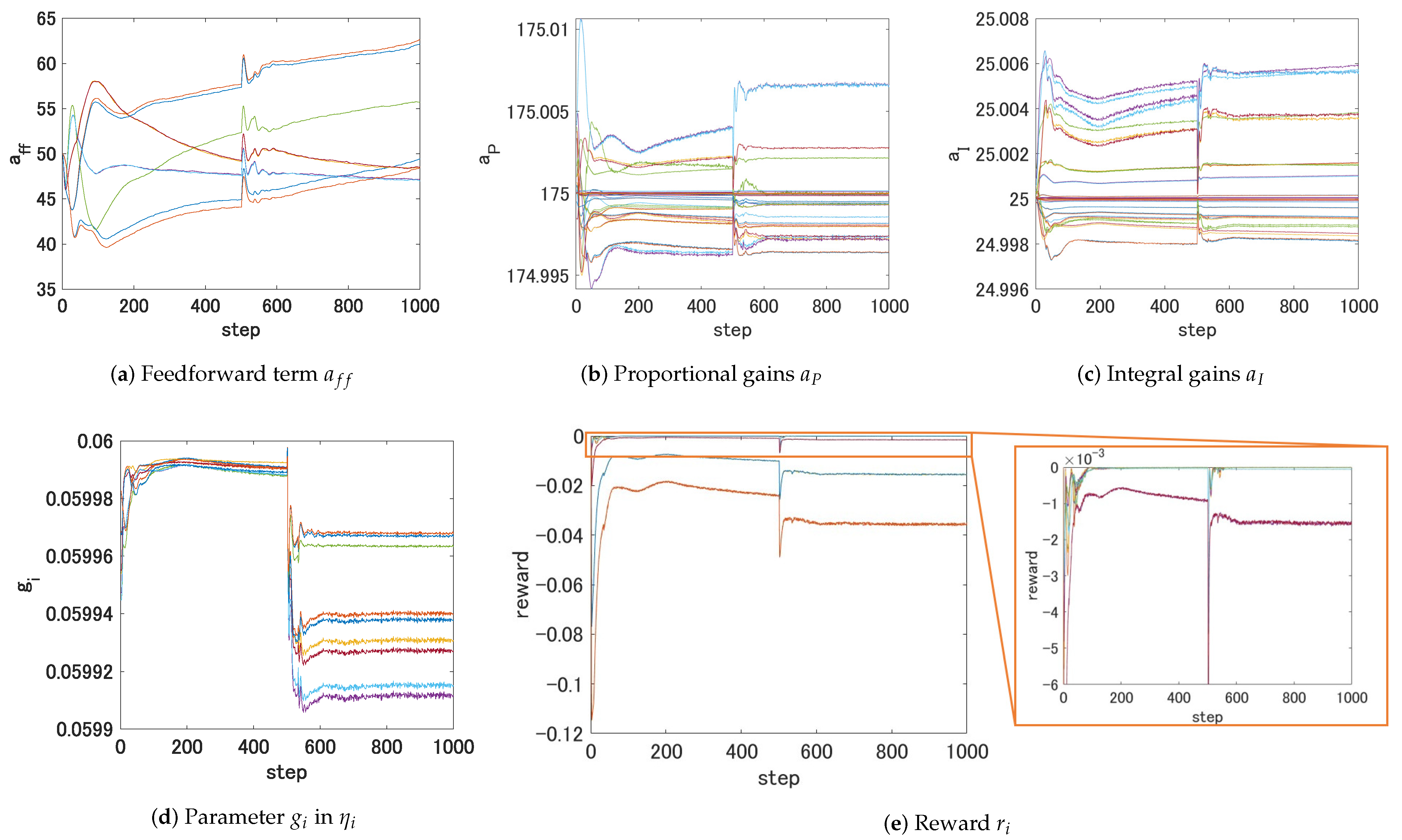
We next show how our proposed controller reacted to the changes of reference. Since the left and the three right devices were excluded as explained earlier in this manuscript, we provide the changes of the controller related parameters of the fourth to twelfth manipulating devices.

All the quantities suffered steep changes at the 500th step. Since 40 episodes of training were completed before applying this scenario, the feedforward control inputs seemed to be dominant in the control behavior, whereas small transient adjustments could be observed in ${\mathit{a}}_P$ and ${\mathit{a}}_I$, as evidenced by the plots in Figure 12. Figure 13 shows the plots corresponding to only the fifth manipulating device. On the changes of PI controller gains, it is of technical interest to note that although $a_{P,5,5}$ and $a_{I,5,5}$ were the largest, the gains corresponding to their closest neighbors ($a_{P,5,*}$ and $a_{I,5,*}$ for $*\in \{4,6\}$) exhibited a similar magnitude, indicating that errors measured at the nearest neighbor devices were important in the control under coupling.

5.3. sRMSE Trajectory under Plant Perturbation

We then introduced perturbations to the dynamics of the manipulating devices. Because the devices were modeled using first-order transfer functions with a lag, we added perturbations to their DC gains and time constants randomly; the perturbed parameters should stay within the interval of $\pm 5\%$ of their nominal values. We note that the perturbation was introduced only in the 41st episode in the self-tuning control scenarios.

We note that the proposed self-tuning controller again exhibited much smaller sRMSE metrics than the static PI controller in this scenario as shown in Figure 14. The use of the adaptive coefficient ${\eta }_{i,j}$ in the self-tuning control system resulted in a continuous improvement in the sRMSE metric after the 400th step, whereas the metric did not decrease with the SISO policy controller.

5.4. Disturbance Rejection

We empirically know that we should sometimes expect a disturbance that would worsen the film thickness precision at the left and right edges. We modeled the disturbance as a perturbation of the thickness around the right edge, which was characterized by:

$$\begin{array}{c}\hfill -3.0exp(-{\left(0.25d_x\right)}^2)(d_x=|50-x|),\end{array}$$

and added it to the thickness after the 500th time step. We did not perturb the plant dynamics in this scenario, and the reference was set to 70 throughout the episode. Figure 15 shows the result.

All three controllers suffered increased sRMSE metrics when a disturbance was introduced. However, the self-tuning controllers quickly rejected the disturbance, whereas the sRMSE metric of the static PI controller continued to decrease even after 500 sampling steps, indicating its very slow transient behavior. Notably, the self-tuning controller with ${\eta }_{i,j}$ defined using (14) showed faster convergence than the SISO self-tuning controller in this scenario, likely because of the spatially monotonic sign of the introduced disturbance.

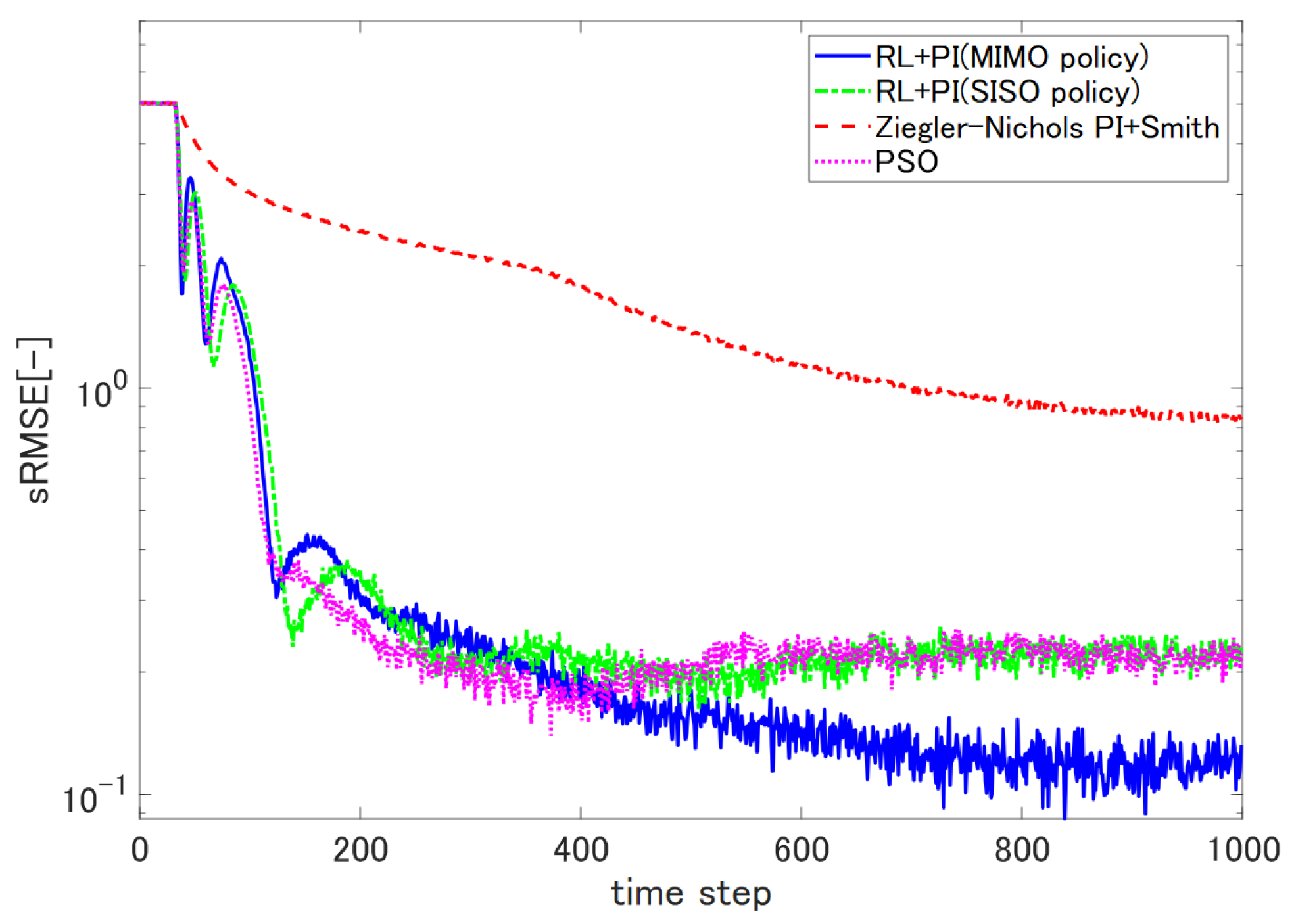
5.5. Comparison with Online Tuning by Particle Swarm Optimization

In order to illustrate the performance enhancement of our proposed control system further, we conducted a comparative on-line tuning of our two-DOF PI controller parameters ${\theta }_{\ast \ast }$ by particle swarm optimization (PSO). PSO is classified as a swarm intelligence algorithm. It can be applied to various global optimization problems, and it is known to exhibit fast convergence.

We tuned the parameters of the proposed two-DOF PI control system in the SISO setup (${\eta }_{i,j}=1$ only if $i=j$; otherwise, it was set to zero). A particle includes all the policy parameters ${\theta }_{**}$, which amounts to a point in the 45th-dimensional space (there are 15 manipulating devices, each of which is assigned a two-DOF PI controller that has three parameters). We prepared 20 initial particles that were distributed within the ±35% range of the initial value. The initial velocities of the particles were randomly initialized within the interval $[-0.5,0.5]$. We needed to define pbest and gbest to evaluate the fitness of the particles (please see [9] for details). We decided to use the sRMSE metric as a fitness evaluation. The updates of the particles were carried out at every 100 steps of episodes, and we performed 40 episodes also for the tuning parameters with PSO. The reference was set to be 70, which was identical to the value used for the numerical evaluation of the proposed control system.

Figure 16 below shows the changes of sRMSE metrics corresponding to the controllers tuned by four different methods. It shows the superior fast adaptation performance of PSO tuning. However, PSO tuning was outperformed by the proposed control system, which explicitly took input coupling into account. It can be said that PSO did not exhibit significant performance improvement over our proposed control system in a SISO setup. We concluded that the proposed control system exhibited not only improved steady-state thickness accuracy, but also comparable learning speed to PSO.

6. Conclusions and Future Work

This study proposes a self-tuning two-DOF PI control system for a MIMO film production process. The adaptive tuning laws of the controller parameters are synthesized based on the actor-critic-type RL algorithm. As the target process intrinsically suffers spatial mechanical coupling, we introduce the tunable coefficient ${\eta }_{i,j}$ to improve the thickness control performance under the existence of spatial couplings of the inputs.

We conduct numerical simulations under several likely scenarios and confirm better control performance compared to that of the conventional static-gain PI controller whose gains are determined using the Z.N. method. The numerical results indicate that the proposed controller exhibits better performance in all likely scenarios.

We observe transient oscillation in the sRMSE thickness error metrics of the proposed control in almost all cases. We will continue to investigate the cause of this phenomenon and will try to synthesize an improved control system with a smaller oscillatory response.

References

1. Morari, M.; Zafiriou, E. Robust Process Control; Prentice Hall: Bergen County, NJ, USA, 1989. [Google Scholar]
2. Desborough, L.; Miller, R. Increasing Customer Value of Industrial Control Performance Monitoring-Honeywell’s Experience. In 6th International Conference Chemical Process Control, AIChE Symp.; Series 326; AIChE: New York, NY, USA, 2002. [Google Scholar]
3. Ogata, K. Modern Control Engineering, 3rd ed.; Prentice Hall: Bergen County, NJ, USA, 1997; p. 669. [Google Scholar]
4. Hägglund, T.; Ȧström, K. Industrial adaptive controllers based on frequency response techniques. Automatica 1991, 27, 599–609. [Google Scholar] [CrossRef]
5. Papadopoulos, K.G.; Tselepis, N.D.; Margaris, N.I. On the automatic tuning of PID type controllers via the Magnitude Optimum criterion. In Proceedings of the 2012 IEEE International Conference on Industrial Technology, Athens, Greece, 19–21 March 2012; pp. 869–874. [Google Scholar] [CrossRef]
6. Sarhadi, P.; Noei, A.R.; Khosravi, A. Adaptive integral feedback controller for pitch and yaw channels of an AUV with actuator saturations. ISA Trans. 2016, 65, 284–295. [Google Scholar] [CrossRef] [PubMed]
7. Acosta, G.; Mayosky, M.; Catalfo, J. An expert PID controller uses refined ziegler and nichols rules and fuzzy logic ideas. J. Appl. Intell. 1994, 4, 53–66. [Google Scholar] [CrossRef]
8. Solihin, M.I.; Tack, L.F.; Kean, M.L. Tuning of PID Controller Using Particle Swarm Optimization (PSO). Int. J. Adv. Sci. Eng. Inf. Technol. 2011, 1, 458–461. [Google Scholar] [CrossRef] [Green Version]
9. Eberhart, R.; Kennedy, J. A new optimizer using particle swarm theory. In Proceedings of the Sixth International Symposium on Micro Machine and Human Science (MHS’95), Nagoya, Japan, 4–6 October 1995; pp. 39–43. [Google Scholar] [CrossRef]
10. Reddy, C.S.; Balaji, K. A Genetic Algorithm (GA)-PID Controller for Temperature Control in Shell and Tube Heat Exchanger. IOP Conf. Ser. Mater. Sci. Eng. 2020, 925, 012020. [Google Scholar] [CrossRef]
11. Han, G.; Fu, W.; Wang, W.; Wu, Z. The Lateral Tracking Control for the Intelligent Vehicle Based on Adaptive PID Neural Network. Sensors 2017, 17, 1244. [Google Scholar] [CrossRef] [PubMed] [Green Version]
12. Spielberg, S.; Gopaluni, R.; Loewen, P. Deep Reinforcement Learning Approaches for Process Control. In Proceedings of the 2017 6th International Symposium on Advanced Control of Industrial Processes (AdCONIP), Taipei, Taiwan, 28–31 May 2017; pp. 201–206. [Google Scholar]
13. Zou, L.; Zhuang, Z.; Cheng, Y.; Huang, Y.; Zhang, W. A new thermal power generation control in reinforcement learning. In Proceedings of the 2018 Chinese Automation Congress (CAC), Xi’an, China, 30 November–2 December 2018; pp. 1734–1739. [Google Scholar] [CrossRef]
14. Fares, A.; Bani Younes, A. Online Reinforcement Learning-Based Control of an Active Suspension System Using the Actor Critic Approach. Appl. Sci. 2020, 10, 8060. [Google Scholar] [CrossRef]
15. Boubertakh, H.; Tadjine, M.; Glorennec, P.Y.; Labiod, S. Tuning fuzzy PD and PI controllers using reinforcement learning. ISA Trans. 2010, 49, 543–551. [Google Scholar] [CrossRef] [PubMed]
16. Wang, X.S.; Cheng, Y.h.; Sun, W. A Proposal of Adaptive PID Controller Based on Reinforcement Learning. J. China Univ. Min. Technol. 2007, 17, 40–44. [Google Scholar] [CrossRef]
17. Sedighizadeh, M.; Rezazadeh, A. Adaptive PID Controller based on Reinforcement Learning for Wind Turbine Control. Proc. World Acad. Sci. Eng. Technol. (CESSE2008) 2008, 27, 257–262. [Google Scholar]
18. Lee, D.; Lee, S.J.; Yim, S.C. Reinforcement learning-based adaptive PID controller for DPS. Ocean Eng. 2020, 216, 108053. [Google Scholar] [CrossRef]
19. Carlucho, I.; De Paula, M.; Acosta, G.G. An adaptive deep reinforcement learning approach for MIMO PID control of mobile robots. ISA Trans. 2020, 102, 280–294. [Google Scholar] [CrossRef] [PubMed]
20. Kimura, H.; Kobayashi, S. An analysis of actor-critic algorithms using eligibility traces: Reinforcement learning with imperfect value functions. J. Jpn. Soc. Artif. Intell. 2000, 15, 267–275. (In Japanese) [Google Scholar]
21. Kamaya, H.; Kitayama, K.; Fujimura, A.; Abe, K. Reinforcement Learning in Continunous State Spaces. In Proceedings of the 229th Workshop of SICE Tohoku Branch, Hachinohe, Japan, 9 June 2006. Document Number 229-11 (In Japanese). [Google Scholar]
Figure 1. Schematic drawing of the film fabrication process.
Processes 09 00487 g001
Figure 2. The location of the manipulating devices over the film width and the positions of the thickness measurements.
Processes 09 00487 g002
Figure 3. Blue broken lines indicate the spatial deformation of the die Ψ x , i while varying i. The red solid plot shows the deformation of the die when the maximum inputs u i ( t ) = 100 are given to all manipulating devices.
Processes 09 00487 g003
Figure 4. Proposed Smith predictor based on the two-DOF PI control system. Its feed-forward control and PI gains are tuned by the RL algorithm. We note that this figure represents the construction of a control system for a single manipulating device, but the reinforcement learning part takes care of the entire process to compensate for the interference between inputs.
Processes 09 00487 g004
Figure 5. Structure of synthesized critic network. It accepts the normalized state vector s to approximate the value function for the i-th manipulating device.
Processes 09 00487 g005
Figure 6. Actor networks for self-tuning controller parameters of the i-th manipulating device. We propose the structure (A) for feedforward control action and (B) for PI control actions. Both networks aim to maximize the expected reward by tuning the parameter θ * , i , j ( * { f f , P , I } ) . As θ * , i , j are functions of their corresponding network parameters v, μ , and σ , we synthesized update rules for those parameters to achieve the goal.
Processes 09 00487 g006
Figure 7. Critic and actor RBF networks for η i , j .
Processes 09 00487 g007
Figure 8. Transient changes in sRMSE metrics calculated with three different controllers.
Processes 09 00487 g008
Figure 9. Changes in sRMSE metrics when the reference thickness is changed from 70 to 65 at the 500th sampling step.
Processes 09 00487 g009
Figure 10. Film thickness distributions at the 500th step corresponding to the Ziegler–Nichols (Z.N.) PI controller and our proposed controller with spatial augmentation.
Processes 09 00487 g010
Figure 11. Changes in sRMSE metrics when the reference thickness is changed from 70 to 75 at the 500th sampling step.
Processes 09 00487 g011
Figure 12. Changes of the quantities related to the self-tuning functionality of the proposed control system under the reference modification scenario.
Processes 09 00487 g012
Figure 13. Changes of the quantities of the fifth manipulating device under the reference modification scenario.
Processes 09 00487 g013
Figure 14. Change in the sRMSE metric for the perturbation of the plant in the 41st episode.
Processes 09 00487 g014
Figure 15. Effect of disturbance on the spatial RMSE metric.
Processes 09 00487 g015
Figure 16. Transient changes in sRMSE metrics calculated with four different controllers.
Processes 09 00487 g016