
Machine Learning Based Optimization Model for Energy Management of Energy Storage System for Large Industrial Park

State Key Laboratory of Pulp and Paper Engineering, South China University of Technology, Guangzhou 510640, China
*
Author to whom correspondence should be addressed.
Processes 2021, 9(5), 825; https://0-doi-org.brum.beds.ac.uk/10.3390/pr9050825
Submission received: 12 March 2021
/
Revised: 28 April 2021
/
Accepted: 28 April 2021
/
Published: 9 May 2021
(This article belongs to the Special Issue Energy Conservation and Emission Reduction in Process Industry)
Abstract
:Renewable energy represented by wind energy and photovoltaic energy is used for energy structure adjustment to solve the energy and environmental problems. However, wind or photovoltaic power generation is unstable which caused by environmental impact. Energy storage is an important method to eliminate the instability, and lithium batteries are an increasingly mature technique. If the capacity is too large, it would cause waste and cost would increase, but too small capacity cannot schedule well. At the same time, the size of energy storage capacity is also constrained by power consumption, whereas large-scale industrial power consumption is random and non-periodic. This is a complex problem which needs a model that can not only dispatch but also give a reasonable storage capacity. This paper proposes a model considering the cycle life of a lithium battery and the installation parameters of the battery, and the electricity consumption data and photovoltaic power generation data of an industrial park was used to establish an energy management model. The energy management system aimed to reduce operating costs and obtain optimal energy storage capacity, which is constrained by lithium battery performance and grid demand. With the operational cost and reasonable battery capacity as the optimization objectives, the Deep Deterministic Policy Gradient (DDPG) method, the greedy dynamic programming algorithm, and the genetic algorithm (GA) were adopted, where the performance of lithium battery and the requirement of power grid were the constraints. The simulation results show that compared with the current forms of energy, the three energy management methods reduced the cost of capacity and operating of the energy storage system by 18.9%, 36.1%, and 35.9%, respectively.
1. Introduction
In recent years, solar energy, a clean and pollution-free renewable energy, has attracted wide attention in various fields. According to the report of International Energy Agency (IEA), generating capacity from renewable energy sources of the world will reach 105 GW by 2020 and 8500 GW by 2050. Although electricity use has fallen sharply as a result of the COVID-2019, renewable energy has escaped the storm because of its higher returns than fossil fuels [1]. The installation and generation data of solar power generation show that solar power generation is a booming industry that successfully competes with fossil fuel power generation and participates in the adjustment of energy structure [2]. However, there is uncertainty and intermittence in solar power generation as well as error in solar power prediction error, which has a great impact on electricity dispatching. Now, with the introduction of the spot market for electricity, industrial companies usually determine the next stage of available power by predicting solar output and demand, then sign agreements with power supply companies based on the forecast data. Due to the error in prediction and some unpredictable factors, purchasing too little or too much electricity often leads to the power shortage or the need to discard a large amount of electricity, resulting in a waste of resources [3].
In order to solve the problem of scheduling and reduce the cost of electricity, the energy storage system (ESS) is applied in the system. ESS is an effective method to solve the electricity scheduling problem of large enterprises as a scheduling element, because it can improve the power utilization rate through energy storage equipment, so as to make up for the inaccurate power prediction and improve the flexibility of the power system [4]. ESS is far superior to conventional thermal power units in both response time and regulation accuracy. In recent years, the ESS has played a critical role in the connection between renewable and fossil energy. The inexhaustible energy provided by photovoltaic plants can be stored in the ESS and used during periods when electricity prices are higher. These storage systems decouple local energy production from consumption. For example, overproduction of local energy can be used in the future until underproduction occurs. However, storage is still used as a buffer to compensate for unpredictable changes. In addition to its strategic value, the global use of electric energy storage systems, especially battery energy storage system (BESS), is still in its infancy due to high investment cost and short service life caused by overuse [5].
A number of studies have been carried out by scholars from different countries. The focus of these studies is to apply battery energy storage system (BESS) to achieve peak shaving of electricity consumption, including the selection of battery capacity and scheduling method. Liu et al. [6] considered the battery life and battery size and used dynamic programming to reduce operating costs. By comparing the costs under different capacities, the optimal capacity of wind power plant was calculated. Elsied et al. [7] proposed an advanced real-time energy management system in order to optimize micro-grid performance in a real-time operation for a distributed power system including photovoltaic, wind generator and fuel cell. Gitizadeh et al. [8] described a battery capacity optimization method. The MIP method was used to calculate the optimal battery capacity. The results showed that the sizing of batteries depends largely on the exact pricing structure. Ke et al. [9] considered the daily charge-discharge control of the BESS and used BESS to balance the peak and off-peak electricity consumption to shave peak loads of different BESS capacities. Prasatsap et al. [10] analyzed the power peak-valley problem of a school, whose fluctuations in energy use caused by winter and summer vacations and added BESS into the school electricity system to adjust the peak. They calculated the equivalent power cost under different capacities and compared it to determine the optimal BESS capacity. Liu et al. [11] proposes an improved non-dominated sorting genetic algorithm-II (INSGA-II) for solving the optimal siting and sizing of distributed generation units.
Other researchers focus on scheduling. In order to solve the optimization of household electrical appliances, Setlhaolo et al. [12] used the method of mixed integer nonlinear programming to realize cost saving by load transfer. They take the equipment coordination into consideration, so that peak load clipping could be further optimized. Wang et al. [13] applied the two operation strategies of BESS suitable for different scenarios to the integrated energy system to balance different energy networks in the co-generation of cold, heat, and electricity, so as to adjust the peak and valley situation of electricity consumption in residential areas. Duman et al. [14] carried out preload scheduling on intelligent thermos and home energy management system to achieve cost minimization, with using BESS to perform power conversion and mixed integer linear programming method. Mehrjerdi et al. [15] adopted BESS as a tool for substation expansion based on Multi-Objective Mixed Integer Linear Programming, considering BESS’s operation in distribution networks to simultaneously substation expansion deferral and cost reduction. Han et al. [16] proposes a novel method combining the simulated annealing algorithm-based Hopfield neural network algorithm (SAA-HNN) and local scheduling rules to solve the production blockage problem.
Deep reinforcement learning also made progress in energy management strategy. Lian et al. [17] put forward a rule-interposing deep reinforcement learning based energy management strategy for power-split hybrid electric vehicle. Compared with energy management strategy based on deep deterministic policy gradient and deep Q learning, the former got a better fuel economy, and the cost reduction was close to dynamic programming method. Chen et al. [18] proposed a personalized battery management strategy based on DDPG algorithm, in order to provide different battery control strategies for users with different preferences.
However, the object of current mainly research is only the power supply side or the power consumption side, rarely considering the demand and impact of both sides on energy management strategy, or the method used cannot adapt to the requirements of users for the spot market of electricity and considering the impact on subsequent dispatching. The rule algorithm is direct and the heuristic method is simple, but in some cases, it is not the best solution [19]. Although the result of DDPG is less stable, but to deal with problems which are difficult to be completely controlled by model-based method with the increasing complexity of energy system, uncertainty, and security problems, it can work without specific model and quickly find solutions [20,21]. In addition, traditional industrial parks often have no ESS or only have little capacity photovoltaic panels. China has not formed a reasonable market trading mechanism, most of the new energy generation can only be used within the region [22].
In conclusion, industrial users need to solve the problems of signing contracts with the spot market and installing energy storage system, so as to achieve the purpose of rational use of electric energy, improving the utilization rate of solar energy, and reducing electricity costs. To solve the scheduling problem of large-scale industrial power consumption, this paper uses machine learning method to calculate the storage capacity and scheduling scheme. Firstly, greedy algorithm is used to get the optimal ESS capacity. Then, the electricity load and photovoltaic power generation were predicted to obtain the daily purchase amount agreed with the spot market of electricity. Next a scheduling model was established to optimize the difference between the forecast and the actual power load. Finally, the optimal scheduling scheme was obtained by comparing the three algorithms.
The work achievements are listed as follows:
- (1)
- The energy management system aimed to reduce power cost and optimize battery capacity.
- (2)
- The integrity of the energy management system was realized by combining prediction and decision-making.
- (3)
- Prediction of renewable energy generation curve with GAN method gave preliminary feedback to the market.
- (4)
- According to decision model based on DDPG method, the system can manage the decision of energy in time.
- (5)
- The energy management framework is estimated by comparing the cost of electricity consumption.
2. Energy Management Framework
2.1. Energy Management System
This paper introduces a complete set of energy management system (EMS), which can guide the automatic control of battery charge and discharge behavior and achieve the purpose of reducing electricity cost. The framework of EMS is shown in Figure 1, it indicates that the photovoltaic power generation and electricity load curve is obtained by prediction model. The prediction model was trained in advance with historical data. Finally, the decision model uses the forecast photovoltaic power generation load curve, the decision-making model of import price, and the control strategy based on machine learning to get the optimal control strategy of battery.
On the previous day, the EMS purchases electric energy from the spot electricity market according to the predicted photovoltaic and electricity load curve, and then the decision model judges the current battery control strategy according to the electric energy purchased the previous day, the predicted future electricity consumption curve, the photovoltaic power generation curve, and the electricity price.
2.2. The Description of Power System of Industrial Park
The focus of the energy management model in this work is the operation planning of the energy storage battery connected with the power system of the industrial park. Figure 1 shows the electric power system of the park. The system includes a lithium battery energy storage system, photovoltaic panels, and converts. The working mode of the system has the following two situations:
- (1)
- The pre-purchased electricity has been able to meet the needs of the park. The photovoltaic power can be stored, and the surplus electricity can be sold to other users in spot market.
- (2)
- The electricity purchased a few days ago cannot meet the needs of the park, so it is necessary to use photovoltaic power or battery discharge or purchase real-time electricity from the spot market to meet the production needs.
- (3)
- The PV produces more electricity than the sum of the battery charge and the load used, and the excess energy is discarded.
To support the above operation mode, ESS installed in the industrial park can reasonably plan the charging or discharging behavior based on the remaining available energy in the battery and the electricity price of the grid. This plan is very important for the park because the electricity will be used for these models.
In the course of operation, the power system of the park is limited by ESS capacity, which will increase the operating cost according to whether there is insufficient or excessive power purchase. In order to find the appropriate ESS capacity and minimize operating costs, an operating cost model was developed. Considering the land cost as well as charging and discharging speed, the battery is selected as the energy storage system device. In addition to the battery energy storage system, flywheel energy storage, capacitor energy storage, and hydraulic energy storage are also solutions of energy storage devices. For the present, lithium battery energy storage is a relatively economical way of energy storage [23,24].
2.3. Problem Formulation
This section defines and quantifies the modules described in Section 2.2, respectively. In this paper, the scheduling problem of EMS is divided into a discrete time problem with a time step of 1 h.
2.3.1. The Declaration Deviation Rate of Electric Power Spot Market
The electricity selling company can return the part of the electric quantity in the long and long-term contract in the spot market that is greater than the electric quantity declared in the market before the day, according to the market price before the day. Therefore, in the calculation of electricity cost, considering the requirement of spot market on the declaration deviation rate, the declaration deviation rate λ0 is set as 50%. If the actual declaration deviation rate λi is higher than λ0, recycle cost is expressed as follows:
If :
If :
where is the weighted average comprehensive electricity price of the whole market node in i-th the hour in the day-ahead market, is the weighted average comprehensive electricity price of the whole market node in the i-th hour in the real-time market, is the electricity consumption declared in i-th hour by the electricity selling company and user in the day-ahead market, is the actual electricity consumption of the user in the i-th hour of the operation day.
2.3.2. Photovoltaic Constraint
The output power of photovoltaic power generation is limited by the weather and the parameters of photovoltaic panels. From the above working modes, it can be seen that when the photovoltaic power generation is greater than the battery charging and electricity load, part of the photovoltaic power generation will be abandoned; when the photovoltaic power generation is greater than the battery charging load, the photovoltaic power generation has to be used in industrial production and part of the electricity should be purchased from the grid. The photovoltaic power satisfies the Equations (3) and (4).
2.3.3. Battery Constraint
Batteries change the energy in the battery by charging and discharging. The following is a simple model of battery charge or discharge energy variation. The time step is defined as 1 h. The model about the battery power variation is defined as:
First the energy in battery does not exceed its capacity at any time.
Then the battery can only charge or discharge.
SOC is used to indicate the ratio of the remaining energy of the battery to the energy after full charge. SOC can be expressed as:
Over-discharging and overcharging can shorten battery life. In order to prevent over charging and over discharging of batteries and extend battery life, the safe use of battery SOC is limited to:
The lower bound of SOC is defined as and as the upper bound of SOC is defined as .
2.3.4. Load Constraint
The electricity load predicted by using historical data and the photovoltaic power generation predicted by using GAN method determine the pre-purchase electricity demand signed by the user and the electricity selling company. The relation between the predict load and the electricity purchased before the day is as follows:
The real-time load is modeled as follows:
is positive when electricity is purchased and negative when electricity is sold.
3. Methodology
In this study, a scheduling optimization model based on PPDG was established to reduce the cost of electric power system in the park and increase the use of environmentally friendly energy. The proposed technical route includes four parts: data collection, data selection, model training, and model evaluation. The GAN algorithm is applied to the data selection part. The greedy strategy, GA and DDPG are presented as comparative cases. Figure 2 shows the electric power system of the industrial park. Figure 3 shows the technical path of this effort.
First of all, the model predicted the electricity load and photovoltaic power generation on the next day. The difference between them is the guide to the demand submitting to the spot market of electricity. Then, the dispatching model is used the next day to adjust the specific power purchase and power consumption mode.
Among them, there are two trading methods in the spot market of power. One is day-ahead and the other is real-time. Users can choose the way to buy power according to their needs. Photovoltaic panels can be either transferred directly to the user through a transformer or stored in a battery system for subsequent transmission at an appropriate time. Whether it is a photovoltaic panel or a battery system, electric energy needs to be treated by a transformer before being used by the user.
This chapter puts forward the system operation cost model. The first section is the calculation formula of the model, the second section is the adjustment and optimization of the model, the third section is simulation results and analysis.
3.1. Operating Cost Model
In order to minimize the cost of power consumption in the park and optimize the ESS output, the optimal capacity size of ESS on the power consumption side of the park was obtained by comparing different operating costs of different ESS capacities.
3.1.1. Construction of System Operating Cost Model
The aim of the model is to obtain the optimal capacity of ESS and minimize the system cost. The objective function is defined as follows:
where J1 is the operating costs include day-ahead power purchase cost, J2 is ESS’s initial investment, J3 is BESS’s operating cost, J4 is solar energy cost, and J5 is real-time power purchase cost.
The forecast model predicts the electricity load of the next day and the photovoltaic power generation load to get the electricity purchase demand for the market. If there is still a gap after the calculation by the scheduling model, it needs to buy in real time from the market.
where uday−1 is day-ahead electricity price, uday0 is real-time electricity price, Pload,predict is the forecasting load, Prest is the quantity to buy from the spot market.
When the SOC of the battery exceeds 90%, the battery cannot continue to charge and the excess electric energy must be discarded. The converted cost of this part of electric energy is as follows:
where usolar is solar energy price, Psolar is the quantity of solar power.
The cost of the battery includes the cost of battery degradation and the cost of the initial battery purchase divided equally throughout the day. The degradation cost of the battery is mainly caused by the irregular charge and discharge during the operation of the system. There are mechanism models and semi-empirical models to explain the cycle life of batteries, but the explanation of mechanism model is complex and difficult to be directly applied in engineering. The semi-empirical model has few parameters, simple calculation, and convenient application. A semi-empirical model proposed by Wang et al. [25] was used to estimate the battery degradation cost, as shown below:
where Qloss is the percentage of capacity loss, B is the pre-exponential factor, Ea is the activation energy in J mol−1, R is the gas constant, T is the absolute temperature, and Ah is the Ah-throughput, which is expressed as Ah = (cycle number) × (depth of discharge) × (full cell capacity), and z is the power law factor. The parameters in Equation (5) with the values shown in Table 1.
Then Equation (5) can be rearranged as followed:
Next, finding the derivative of Ah in Equation (5) yields then following:
Combining Equations (5)–(7) over time step from t to t + 1 yields the following:
Finally, the operating costs of the battery can be represented as follows [26]:
where Cbat is the total capacity of ESS, pricebat is the price of battery.
This paper focused on the performances of ESS, the accuracy of the battery is not very important. The battery Rint model can meet the requirements, and at the same time reduce the complexity of calculation. The Rint model included battery ideal voltage source Uoc and ideal battery internal resistance Ro. The battery Rint model is shown in Figure 4.
The operating cycle of the ESS was set at 10 years without calculating the cost of the battery floor space [27]. Therefore, the average hourly purchase cost of the ESS is described as follows:
where t is the operating hours.
3.1.2. Optimization Objectives and Constraints
The difference between electricity bought a day in advance and actual load is defined as demand power Pdemand. When the demand power is greater than zero, extra electricity bought in advance can be sold to other users. On the contrary, purchase of electricity, battery discharge, and photovoltaic power are three options. The choice of optimization step of the model directly affects the size of the optimal result. Solar power is a volatile source of electricity, for it is hard to predict when dark clouds drift across, but photovoltaic curves circulate roughly in days. The short-term solar power prediction techniques (0–24 h) are used to dispatch, establish agreements on trading power in certain power market. This paper set an optimization step size to 1 h [28,29].
The constraints of the above optimization function are as follows:
- (1)
- Output power constraint
- (2)
- Charge constraint
- (3)
- Discharge constraint
BESS is composed of battery cells whose properties are constrained by a single cell. Considering the impact of capacity on battery life, the ESS capacity should be kept within a range at all times. BESS can choose to charge or discharge. Due to the structure of the system, the upper limit of charge is the electric energy generated by the photovoltaic panel during this period, and the upper limit of discharge is the battery capacity.
3.2. Optimization for Capacity of ESS and Dispatch Strategy
In recent years, many studies have been conducted on ESS energy management algorithms used to solve industrial problems. Among these methods, the more common method is to use detailed partition to obtain the best solution such as dynamic programming algorithm or use heuristic algorithm to search the best solution [30]. The scenarios in this paper require a prediction of future electricity use, thus a lot of historical experience is needed to guide decisions. For the DP method, the rules are made artificially, there are certain limitations and global optimization cannot be achieved. Moreover, for a scheduling model that is influenced by both the electricity selling company and the users, the rules are not transparent. Heuristic algorithm is simple and intuitive, but when the data dimension reaches a certain degree, it will cause great computational pressure and it is difficult to achieve good results [31]. Reinforcement learning does not require model input, and the calculation speed is fast, but it is difficult to achieve convergence [32]. To this end, this paper selects three methods based on rule, GA and DDPG to carry out the inverse and comparison.
3.2.1. Energy Management Based on Greedy Rules
Greedy rules shown in Figure 5 is used for energy management. The difference between electricity bought a day in advance and actual load is defined as demand power Pdemand. The working mode is described as follows:
- (1)
- When Pdemand ≥ 0, the day-ahead purchase has met the demand and the excess energy needs to be sold to other users and the ESS charge.
- (2)
- When Pdemand < 0, the available storage energy of the ESS and energy generated by photovoltaic plants can meet Pdemand, consumed the energy generated by photovoltaic plants first and then the ESS discharge.
- (3)
- When Pdemand < 0 and the available storage energy of the ESS and energy generated by photovoltaic plants cannot meet Pdemand, the system needed to buy additional power from market to meet the demand of the industrial park.
3.2.2. Energy Management Based on Genetic Algorithm
Genetic algorithm (GA) is an intelligent optimization algorithm that simulates the evolution process of natural organisms. It seeks the optimal solution by constantly generating offspring. In this paper, the percentage of the ESS output power at this time is taken as an individual in the genetic algorithm, as shown in the formula:
where, P is the charge and discharge of the battery at each point in time.
The fitness function of this algorithm is:
where un is the operating cost of the system using energy management based on GA method.
3.2.3. Energy Management Based on Deep Deterministic Policy Gradient
The depth deterministic policy gradient is a method that calculate the state with the neural network to get the selected action, perform the action to get the new state and reward, and then put the sample into the experience playback pool for neural network training. It does not need model input and can deal with high dimensional space quickly. Deterministic policy is compared with random strategy. For some action set, it may be continuous value or very high dimensional discrete value, so the space dimension of action is very large. In this case, the matrix is superior [33,34].
The basic algorithm implementation framework of DDPG is shown in Figure 7. This paper realized the calculation of DDPG method through the following steps:
- (1)
- Determine the time interval for model calculation: select 1 h as the time interval.
- (2)
- Determine which state variables were selected: The problem is represented at each stage by a set of different states, including purchased electricity, day-ahead price, real-time electricity price, actual electricity consumption, photovoltaic power generation quantity, and ESS capacity.
- (3)
- Determine decision variables and transition equations: State transitions are determined by states and actions based on previous state. In this work, the decision variable is ESS discharge. The state transfer equation of ESS capacity variable is:where SOC(t) is the proportion of electric energy in the battery’s capacity at time t, Pbat(t − 1) is the charge or discharge at time t.
- (4)
- Determine the objective function applicable to the DDPG algorithm: the objective function is set as follows:
The actor–critic framework adopted by DDPG is a process of iterative training of policy networks and Q networks through the interaction of the environment, actor, and critic in the context of recurring plots and time steps. The experience pool, the double actor networks and the double critic networks are the three important parts of DDPG. When actor network interactions with the environment, the resulting transformation data sequence is highly temporal. If these data sequences are used directly for training, the neural network will overfit and not easily converge. The actor network in the framework stores the transformed data into the storage space firstly and then randomly samples small batch data from the storage space during training so that the sampled data can be treated as irrelevant data. The policy gradient gives the actions that should be taken in a given state. Actor network is policy functions that generate actions and interact with the environment. Actor target network selects the optimal action A ‘according to the next state S’ sampled in the empirical playback pool and the parameter θ’ is copied periodically from actor network. Critic network uses the value function, which evaluates the performance of actors and guides them to the next stage of action. Critic target network is responsible for calculating Q value of sample selected from empirical playback pool.
The algorithm flow is shown as follows:
Iteration algorithm input: critic network structure, critic target network structure, actor network structure, and actor target structure and their parameters θ, θ′, w, w′, train episode T, state characteristic dimension n, gamma attenuation factor γ, soft update coefficient τ, batch gradient descent sample number m, target Q network parameter update frequency C, random noise function. The parameters are shown in Table 3.
Output: Actor network parameter θ, Critic network parameter w.
- (1)
- Randomly initializes the parameter θ, θ′, w, w′, thereinto, θ = θ′, w = w′. Clear set of experience playback.
- (2)
- For i from 1 to T:
- Initialization S for the sequence of the current state of the first state, get its eigenvector ϕ (S).
- Based on actor network, use ϕ(S) as input, action A as output, get new state S′ and feedback R. Judge it is terminated or not (is_end is true or false).
- Store {ϕ(S), A, R, ϕ(S′), is_end} in the experience playback set D.
- S = S′
- Sampling m samples from the playback experience set D, {ϕ (Sj), Aj, Rj, ϕ (S′j), is_endj}, j = 1, 2, …, m, calculating Q value yj.
- The mean square error loss function is used for the gradient update of the parameter W of the critic network.
- Update Actor network parameter θ.
- If T%C = 5, update the critic target network and actor target network parameters.
- If is_end is true, the current iteration completes, otherwise go to step b.
3.3. Prediction Model of PV Generation and User Load Power
3.3.1. PV Generation Prediction
GAN consists of a generator and a discriminator. As shown in Figure 8, the generator attempts to generate a sample that is close to the real data with a given variable vector Z, while the goal of the discriminator is to distinguish the sample from the real historical data and the generated data. In the process of training, they compete and make process together. The loss function of a GAN is as follows:
where D(x) is the probability of a picture generated by discriminator id a real picture, D(G(x)) is the probability of discriminator judging whether the picture generated by generator is real, E is the expectation of the given random variables, Pdata is the distribution of the true historical data, and Pz is the distribution of noise vector, which follows a Gaussian distribution.
The purpose of the discriminator is to form a differentiable function to classify the input data. When false data entered, the discriminator expects to output 0, and when real data entered, the discriminator outputs 1. A multilayer perceptron with one hidden layer h1 including 150 neurons was chosen as discriminator, and the generator was designed by LSTM with its strong ability in time series data. The data of the last 15 days at the same time was chosen to predict the PV generation. Suppose the input is X consisting data of t days, each xt in X is a vector and is composed of 15 features. In the generator, a fully connected layer with 15 neurons is put into generate x′ which aims to approximate real data to spoof discriminator.
3.3.2. User Load Power Prediction
For a user who has regular power consumption, the simple averaging (SA) strategies have also been shown to be highly competitive in applications [35]. In this work, the average of load power in last 7 days at the same time was chosen as the load power prediction data.
4. Case Studies
4.1. Data and Assumptions Required
An industrial park with a photovoltaic power center is selected for studies. Typical data were selected from the historical data, and then the predicted reference load data were output by GAN method and SA method, and compared with the actual output, as shown in Figure 9 and Figure 10.
The generated forecasting error of GAN and SA models for the PV load and electricity consumption are presented in Table 4. It can be seen that the PV prediction error is relatively large, this is related to weather change and the amount of data. This work mainly focuses on the following energy management, and the inaccurate prediction data is a problem to be solved.
Further, the price of photovoltaic power is selected to be 0.35 RMB/kWh [36] and sets the efficiency of the converter in the system to 95%. Electricity price and spot market electricity price come from the price announced by power grid and historical bidding in spot market, and the current grid price is 0.638 RMB/kWh. Considering that excessive discharge depth will accelerate the replacement of the battery, the available range of the battery is set to 10–90% of its SOC and initial phase, and 10% of the SOC of the battery termination phase [6]. Considering the real-time balance of electric energy, we will sell the surplus electricity at half price. The proposed EMS model is verified to be feasible by comparing the four scenarios. In scenario A, B, and C, the user adopts the greedy, GA, and DDPG dispatch model, respectively, and wants to get the maximum profit under the condition of suitable SOC of battery. In scenario D, the user does not adopt any dispatch model and just purchases power on the day on the spot market.
Photovoltaic data predicted by GAN prediction model and electricity load data predicted by SA prediction model are used in all the four scenes. Meanwhile, in order to ensure consistency, the same parameter processing is carried out for each model.
4.2. Case Studies
The predicted and actual load data in Figure 9 and Figure 10 were imported into EMS for training, to generate the optimal control strategy for the forecast week. In order to get the optimal battery capacity, the operating cost of the battery capacity was assumed to ensure that all photovoltaic power is not wasted without limiting the battery capacity. The three strategies in scenarios for the predicted data and the reference data are shown in Figure 11. The change curve of battery power is shown in Figure 12. It can be seen that the power consumption of the industrial park is regular. The electricity charge during 0:00–8:00 is lower, and the load power required by users is relatively small compared with other periods. During the period of 9:00–13:00, the battery will have a low power discharge, and the power supply from the grid will meet the remaining power demand. In the two cases, the price of power grid is relatively cheap and the output of photovoltaic is relatively small, so appropriate electricity is purchased from power grid to meet the requirement. In the period of 14:00 to 17:00, the electricity price reaches the peak in the period of 14:00 to 17:00, which is also the peak of power consumption. At this time, the battery is released, reducing the power consumption of the day. At other times, because the power in the battery has been consumed and no new photovoltaic energy is generated, the curve is flat. In the model, the weekly minimum reward is taken as the training objective. Although the strategies of the three energy management models are different, the overall trend is the same, using the lowest cost of electricity as far as possible to meet the economic requirements of users.
The change of money at each moment is shown in Figure 13. The three energy management methods, Greedy, GA, and DDPG can effectively optimize the operating cost of the system, and not participating in the spot market rules will greatly increase the operating cost. The greedy method stores as much energy as possible to satisfied the next possible energy shortage, but the utilization rate of battery is not high. Due to the limitation of the genetic algorithm, it is difficult to get the global optimal solution. Although DDPG algorithm is less stable than GA, it is easier to get the global optimal solution than GA.
At the end of the forecast week, compared with the actual operating cost, the total weekly costs of the three method differ by RMB 90,562.79, 86,563.57, and 87,185.52. Compared with the operating cost of no agreement ahead and buying electricity on the same day, the three methods differ by RMB 4461.56, 462.33, and 1084.28. However, at the same time, the curve trend of the battery capacity and the operating cost of the three methods was opposite. Therefore, first of all, we considered the data is not typical or the experimental time is too short.
A month was selected as a forecast period. The battery power curve is shown in Figure 14 and the change of money in each moment is shown in Figure 15. It can be seen that at the end of forecast month, the Greedy method does not consider the long-term energy demand, resulting in a lot of energy is only stored in the battery but not used. This is a waste of energy and the operating cost is rising. The relationship between the battery capacity and the operating cost of the three methods was consistent.
According to above results, Figure 16 shows the optimal change of the lowest electricity cost of the BESS based on the greedy method for different battery capacity Cbat values. More specifically, Figure 15 shows the action and money with battery capacity ranging from 200 to 1200 kWh. It can be seen that when Pdemand is greater than zero, the BESS is properly charged to meet the subsequent energy needs. Limited by the capacity of batteries system, there are moments when not all needs can be met, but as the capacity of the BESS increases, the range of load requirements can be satisfied also increases. When the capacity of BESS is enough, but charge or discharge power is insufficient, then there is no change in the optimized electricity curve, but the operating cost will keep on increasing if it continues to increase energy storage capacity. In the ideal situation, the storage system can supply energy every time the real-time price is high, but this always requires a large capacity. Given the cost of buying and maintaining operating batteries, the benefits must be balanced against the cost of generating and storing energy. It is important to make sure that the best battery capacity is selected.
The results in Figure 13 show that the current battery cost is too high, and the reduced cost of using energy storage equipment and photovoltaic energy cannot offset the cost of battery purchase and maintenance, so the electricity cost has been rising. Figure 14 calculates the relationship between electricity cost and energy storage capacity under different battery costs.
Figure 17 shows the monthly operating cost (RMB) of the BESS using the greedy energy management when the calculated BESS capacity (kWh). It can be observed that when energy storage is free, the operating cost will decrease at the beginning, and it will not decrease when the capacity of batteries reaches a certain extent. When the price reaches a certain level, the cost of purchasing battery is higher than the benefit brought by dispatching. At this time, the lowest operating cost is achieved without using batteries. According to the Energy Information Administration (EIA), the average cost of battery storage capacity in the United States has fallen from USD 2152 in 2015 to USD 625 in 2018. The price of unit capacity is selected to 1000 RMB/kWh [37].
According to the simulation data, we can conclude that when the capacity of BESS increases to about 1600 kWh, the increased capacity can no longer continue to reduce the cost. It can be seen that with the increase of unit energy storage cost, the capacity that can meet the lowest operating cost becomes lower and lower until the operating cost is the lowest when the energy storage is not used. However, the current energy storage cost price is still high for the target park. When the energy storage cost is lower than 318.85 RMB/kWh, using energy storage can reduce the operating cost.
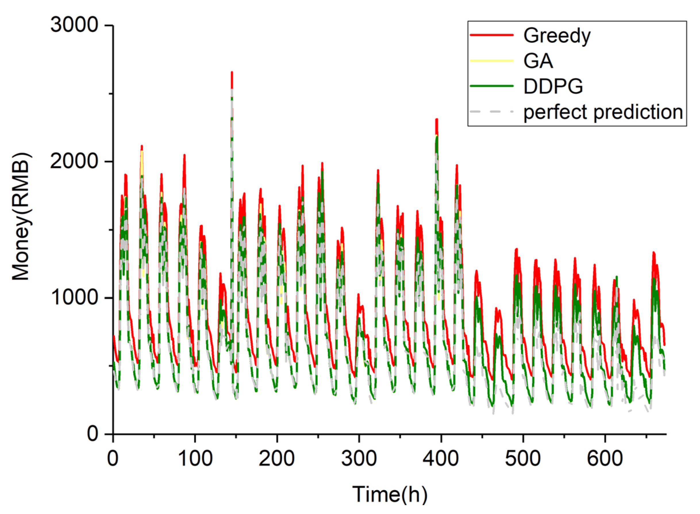
Figure 18 shows the impact of the accuracy of the forecast of electricity load and photovoltaic generation on the reduction of electricity cost. Assuming that the predicted value is exactly equal to the actual value, then the real-time purchase of electricity is equal to the amount of excess electricity returned to the market and the charge and discharge action of the battery.
It can be seen from the Figure 18 that perfect prediction can reduce electricity cost, but there are many factors that affect the prediction result. The question discussed in this paper is whether scheduling can still reduce electricity cost if the prediction result is not so accurate.
5. Conclusions
This paper proposes a battery management strategy based on the combination of GAN prediction and DDPG scheduling to optimize the power consumption for the users who have power generation devices and want to reduce the power consumption cost. Specifically, the user signed an agreement with the spot market according to the forecast results, and then the energy is distributed according to the actual situation of the day. Compared with the greedy algorithm and the genetic algorithm, DDPG has a continuous operating space, and it is not easy to fall into the local optimal solution when exploring the global optimal solution.
In this paper, four scenarios are introduced to calculate operating costs to verify the proposed model. The results show that without considering the cost of battery, greedy energy management method, GA energy management method, and DDPG energy management method can reduce the capacity and operating cost of the energy storage system by 18.9%, 36.1% and 35.9%, respectively, compared by current electricity costs. Even if there is an error between the predicted results and the actual results, the pre-training optimization operation can still achieve satisfactory results. The calculation also shows that the current price of lithium battery is too high, and the use of energy storage system cannot reduce the operating cost in the case study. Only when the unit price of lithium battery is reduced to 318 RMB/kWh, can the operating cost be reduced. The current price is not suitable for the use of energy storage. The results show that the DDPG model established in this paper can solve the scheduling problem of large industrial park as well as calculate the energy storage capacity, and the operation cost is close to the GA method.
In the mode adopted in this paper, the energy storage mode only receives the photovoltaic power generation panel and does not consider the grid energy storage into the battery. The goal of reducing the electricity bill considered in this paper is only a daily optimization goal. These conditions limit the performance of the model. In the future, the connection between energy storage and different energy sources should be taken into account, and the power loss during the conversion process should be taken into account, so as to finally establish a more complete energy management model. At the same time, models should be trained and evaluated on a monthly and annual basis, and different user preferences should be considered to make the framework proposed in this paper more generally applicable.
Author Contributions
Methodology, Y.G.; writing—original draft preparation, Y.G.; writing—review and editing, J.L.; supervision, M.H. All authors have read and agreed to the published version of the manuscript.
Funding
This research received no external funding.
Institutional Review Board Statement
Ethical review and approval were waived for this study, due to for studies not involving humans or animals.
Informed Consent Statement
Not applicable.
Data Availability Statement
The data presented in this study are available on request from the corresponding author. The data are not publicly available due to business secret.
Conflicts of Interest
The authors declare no conflict of interest.
References
- Kuzemko, C.; Bradshaw, M.; Bridge, G. Covid-19 and the politics of sustainable energy transitions. Energy Res. Soc. Sci. 2020, 68, 101685. [Google Scholar] [CrossRef]
- Tschopp, D.; Tian, Z.Y.; Berberich, M. Large-scale solar thermal systems in leading countries: A review and comparative study of Denmark, China, Germany and Austria. Appl. Energy 2020, 270, 114997. [Google Scholar] [CrossRef]
- Mehrjerdi, H. Simultaneous load leveling and voltage profile improvement in distribution networks by optimal battery storage planning. Energy 2019, 181, 916–926. [Google Scholar] [CrossRef]
- Sakti, A.; Gallagher, K.G.; Botterud, A. Enhanced representations of lithium-ion batteries in power systems models and their effect on the valuation of energy arbitrage applications. J. Power Sources 2016, 342, 279–291. [Google Scholar] [CrossRef]
- Pierpoint, L.M. Harnessing electricity storage for systems with intermittent sources of power: Policy and R&D needs. Energy Policy 2016, 96, 751–757. [Google Scholar]
- Liu, Y.; Wu, X.G.; Du, J.Y. Optimal sizing of a wind-energy storage system considering battery life. Renew. Energy 2019, 147, 2470–2483. [Google Scholar] [CrossRef]
- Elsied, M.; Oukaour, A.; Gualous, H. Optimal economic and environment operation of micro-grid power systems. Energy Convers. Manag. 2016, 122, 182–194. [Google Scholar] [CrossRef]
- Gitizadeh, M.; Fakharzadegan, H. Battery capacity determination with respect to optimized energy dispatch schedule in grid-connected photovoltaic (PV) systems. Energy 2014, 65, 665–674. [Google Scholar] [CrossRef]
- Ke, B.R.; Ku, T.T.; Ke, Y.L. Sizing the battery energy storage system on a university campus with prediction of load and photovoltaic generation. IEEE Trans. Ind. Appl. 2016, 52, 1136–1147. [Google Scholar]
- Prasatsap, U.; Kiravittaya, S.; Polprasert, J. Determination of Optimal Energy Storage System for Peak Shaving to Reduce Electricity Cost in a University. Energy Procedia 2017, 138, 967–972. [Google Scholar] [CrossRef]
- Liu, W.; Luo, F.M.; Liu, Y.L. Optimal siting and sizing of distributed generation based on improved nondominated sorting genetic Algorithm II. Processes 2019, 7, 955. [Google Scholar] [CrossRef] [Green Version]
- Setlhaolo, D.; Xia, X.H. Optimal scheduling of household appliances with a battery storage system and coordination. Energy Build. 2015, 94, 61–70. [Google Scholar] [CrossRef]
- Wang, Y.L.; Qi, C.Y.; Dong, H.R. Optimal design of integrated energy system considering different battery operation strategy. Energy 2020, 212, 118537. [Google Scholar] [CrossRef]
- Duman, A.C.; Erden, H.S.; Gönül, O. A home energy management system with an integrated smart thermostat for demand response in smart grids. Sustain. Cities Soc. 2020, 65, 102639. [Google Scholar] [CrossRef]
- Mehrjerdi, H.; Rakhshani, E.; Iqbal, A. Substation expansion deferral by multi-objective battery storage scheduling ensuring minimum cost. J. Energy Storage 2019, 27, 101119. [Google Scholar] [CrossRef]
- Han, Z.H.; Han, C.; Lin, S. Flexible flow shop scheduling method with public buffer. flexible flow shop scheduling method with public buffer. Processes 2019, 7, 681. [Google Scholar] [CrossRef] [Green Version]
- Lian, R.Z.; Peng, J.K.; Wu, Y.K. Rule-interposing deep reinforcement learning based energy management strategy for power-split hybrid electric vehicle. Energy 2020, 197, 117297. [Google Scholar] [CrossRef]
- Chen, P.Z.; Liu, M.C.; Chen, C.X. A battery management strategy in microgrid for personalized customer requirements. Energy 2019, 189, 116245. [Google Scholar] [CrossRef]
- Ei-Sayed, W.T.; EI-Saadany, E.F.; Zeineldin, H.H. Fast initialization methods for the nonconvex economic dispatch problem. Energy 2020, 201, 117635. [Google Scholar] [CrossRef]
- Perera, A.T.D.; Kamalaruban, P. Applications of reinforcement learning in energy systems. Renew. Sustain. Energy Rev. 2020, 137, 110618. [Google Scholar] [CrossRef]
- Yang, T.; Zhao, L.Y.; Li, W. Reinforcement learning in sustainable energy and electric systems: A survey. Annu. Rev. Control 2020, 49, 145–163. [Google Scholar] [CrossRef]
- Liu, S.Q.; Yang, Q.; Cai, H.X. Market reform of Yunnan electricity in southwestern China: Practice, challenges and implications. Renew. Sustain. Energy Rev. 2019, 113, 109265. [Google Scholar] [CrossRef]
- Zakeri, B.; Syri, S. Electrical energy storage systems: A comparative life cycle cost analysis. Renew. Sustain. Energy Rev. 2015, 42, 569–596. [Google Scholar] [CrossRef]
- Sun, L.; Li, G.R.; You, F.Q. Combined internal resistance and state-of-charge estimation of lithium-ion battery based on extended state observer. Renew. Sustain. Energy Rev. 2020, 131, 109994. [Google Scholar] [CrossRef]
- Wang, J.; Liu, P.; Hicks-Garner, J. Cycle-life model for graphite-LiFePO4 cells. J. Power Sources 2011, 196, 3942–3948. [Google Scholar] [CrossRef]
- Beltran, H.; Cardo-Miota, J.; Segarra-Tamarit, J. Battery size determination for photovoltaic capacity firming using deep learning irradiance forecasts. J. Energy Storage 2020, 33, 102036. [Google Scholar] [CrossRef]
- Li, J.H.; Zhang, Z.S.; Shen, B.X. The capacity allocation method of photovoltaic and energy storage hybrid system considering the whole life cycle. J. Clean. Prod. 2020, 275, 122902. [Google Scholar] [CrossRef]
- Rafati, A.; Joorabian, M.; Mashhour, E. High dimensional very short-term solar power forecasting based on a data-driven heuristic method. Energy 2020, 219, 119647. [Google Scholar] [CrossRef]
- Wood, D.A. Hourly-averaged solar plus wind power generation for Germany 2016: Long-term prediction, short-term forecasting, data mining and outlier analysis. Sustain. Cities Soc. 2020, 60, 102227. [Google Scholar] [CrossRef]
- Lupangu, C.; Bansal, R.C. A review of technical issues on the development of solar photovoltaic systems. Renew. Sustain. Energy Rev. 2017, 73, 950–965. [Google Scholar] [CrossRef]
- Lu, X.H.; Zhou, K.L.; Zhang, X.L. A systematic review of supply and demand side optimal load scheduling in a smart grid environment. J. Clean. Prod. 2018, 203, 757–768. [Google Scholar] [CrossRef]
- Wu, T.; Wang, J.H. Artificial intelligence for operation and control: The case of microgrids. Electr. J. 2021, 34, 106890. [Google Scholar]
- Hao, R.; Lu, T.G.; Ai, Q. Distributed online learning and dynamic robust standby dispatch for networked microgrids. Appl. Energy 2020, 274, 115256. [Google Scholar] [CrossRef]
- Liu, Y.N.; Guan, X.; Sun, D. Evaluating smart grid renewable energy accommodation capability with uncertain generation using deep reinforcement learning. Future Gener. Comput. Syst. 2020, 110, 647–657. [Google Scholar] [CrossRef]
- Blanc, S.M.; Setzer, T. When to choose the simple average in forecast combination. J. Bus. Res. 2016, 69, 3951–3962. [Google Scholar] [CrossRef]
- Jiang, H.; Jin, Y.M.; Ye, X. Review of China’s PV industry in 2019 and prospect in 2020. Sol. Energy 2020, 3, 14–23. [Google Scholar]
- Zhang, Y.X.; Li, Z.D. A comparative analysis of the price changes of lithium-ion battery for electric vehicles in China and Japan based on the learning curve model. Energy China 2020, 8, 32–35. [Google Scholar]
Figure 1.
Framework of Energy Management.

Figure 2.
ESS System Structure of the Industrial Park.

Figure 3.
The Flow Chart of the Dispatching Model.

Figure 4.
The battery Rint model.

Figure 5.
Flow Chart of Greedy Rules.

Figure 6.
Flow Chart of GA method.

Figure 7.
Flow Chart of DDPG method.

Figure 8.
Flow Chart of GAN method.

Figure 9.
GAN-based prediction PV generation power curve and actual generation power curve.

Figure 10.
SA-based prediction load power curve and actual load power curve.

Figure 11.
Energy of charge and discharge of energy management experiments.

Figure 12.
Battery power curve of energy management experiments.

Figure 13.
Change of money of energy management experiments.

Figure 14.
Battery power curve of energy management experiments.

Figure 15.
Change of money of energy management experiments.

Figure 16.
Optimal action and money for different BESS capacities. (a) 200 kWh; (b) 400 kWh; (c) 600 kWh; (d) 800 kWh; (e) 1000 kWh; (f) 1200 kWh.
Figure 16.
Optimal action and money for different BESS capacities. (a) 200 kWh; (b) 400 kWh; (c) 600 kWh; (d) 800 kWh; (e) 1000 kWh; (f) 1200 kWh.

Figure 17.
Optimal operating costs of the BESS given different capacity and price of unit capacity.

Figure 18.
Change of money of perfect prediction and other methods.


Table 1.
LiFePO4 battery degradation model calibration parameters corresponding to Equation (23).
| Parameter (Unit) | Value |
|---|---|
| B | 30,330 |
| Ea (J/mol) | 31,500 |
| z | 0.552 |
| R (J/(mol×K)) | 8.314 |
| T (K) | 298 |
Table 2.
Parameters of GA method in this paper.
| Parameter | Value |
|---|---|
| Population size | 500 |
| Crossover fraction | 0.9 |
| Migration fraction | 0.1 |
| generation | 2000 |
Table 3.
Parameters of DDPG method in this paper.
| Parameter | Value |
|---|---|
| Train episode | 1000 |
| State characteristic dimension | 7 |
| Gamma attenuation factor | 1.0 |
| Soft update coefficient | 0.001 |
| Batch gradient descent sample number | 128 |
| Target Q parameter update frequency | 5 |
| Variance of random noise | 0.05 |
Table 4.
Parameters of DDPG method in this paper.
| Cases | MAE | MAPE | RMSE |
|---|---|---|---|
| GAN for PV | 28.603 | 0.709 | 57.156 |
| SA for electricity consumption | 245.583 | 0.183 | 543.95 |
Publisher’s Note: MDPI stays neutral with regard to jurisdictional claims in published maps and institutional affiliations. |
© 2021 by the authors. Licensee MDPI, Basel, Switzerland. This article is an open access article distributed under the terms and conditions of the Creative Commons Attribution (CC BY) license (https://creativecommons.org/licenses/by/4.0/).
Share and Cite
MDPI and ACS Style
Gao, Y.; Li, J.; Hong, M. Machine Learning Based Optimization Model for Energy Management of Energy Storage System for Large Industrial Park. Processes 2021, 9, 825. https://0-doi-org.brum.beds.ac.uk/10.3390/pr9050825
AMA Style
Gao Y, Li J, Hong M. Machine Learning Based Optimization Model for Energy Management of Energy Storage System for Large Industrial Park. Processes. 2021; 9(5):825. https://0-doi-org.brum.beds.ac.uk/10.3390/pr9050825
Chicago/Turabian StyleGao, Ying, Jigeng Li, and Mengna Hong. 2021. "Machine Learning Based Optimization Model for Energy Management of Energy Storage System for Large Industrial Park" Processes 9, no. 5: 825. https://0-doi-org.brum.beds.ac.uk/10.3390/pr9050825
Note that from the first issue of 2016, this journal uses article numbers instead of page numbers. See further details here.