
Health and Housing Energy Expenditures: A Two-Part Model Approach


1
Faculty of Engineering (FEUP), University of Porto, 4200-026 Porto, Portugal
2
ALGORITMI Research Centre, School of Engineering Campus de Azurém, University of Minho, 4800-058 Guimarães, Portugal
3
Department of Mechanical Engineering, Faculty of Engineering (FEUP), Institute of Science and Innovation in Mechanical Engineering and Management Engineering (INEGI), University of Porto, 4200-465 Porto, Portugal
*
Author to whom correspondence should be addressed.
Processes 2021, 9(6), 943; https://0-doi-org.brum.beds.ac.uk/10.3390/pr9060943
Submission received: 14 April 2021
/
Revised: 21 May 2021
/
Accepted: 22 May 2021
/
Published: 27 May 2021
(This article belongs to the Special Issue Renewable Energy Technologies and Systems: Technical, Environmental, Economic, Social, and Cultural Challenges)
Abstract
:Interest in the interaction between energy and health within the built environment has been increasing in recent years, in the context of sustainable development. However, in order to promote health and wellbeing across all ages it is necessary to have a better understanding of the association between health and energy at household level. This study contributes to this debate by addressing the case of Portugal using data from the Household Budget Survey (HBS) microdata database. A two-part model is applied to estimate health expenditures based on energy-related expenditures, as well as socioeconomic variables. Additional statistical methods are used to enhance the perception of relevant predictors for health expenditures. Our findings suggest that given the high significance and coefficient value, energy expenditure is a relevant explanatory variable for health expenditures. This result is further validated by a dominance analysis ranking. Moreover, the results show that health gains and medical cost reductions can be a key factor to consider on the assessment of the economic viability of energy efficiency projects in buildings. This is particularly relevant for the older and low-income segments of the population.
1. Introduction
Interest in the interaction between energy and health within the built environment has been increasing in recent years, in the context of climate change and sustainable development. Recent studies focusing on overheating, cold homes and the inability of households to keep comfortable indoor temperatures [1,2,3,4,5,6], have emphasized the exposure to inadequate indoor temperatures. According to Daniel et al., the issue of cold homes has been increasingly recognized even in mild climate countries, with households in Adelaide registering indoor temperatures below health thresholds and low indoor thermal comfort perception [2]. A recent study by Guertler and Smith on cold homes reports that the majority of excess winter mortality in the United Kingdom (UK) is linked to the “the coldest 25% of homes in the UK” and to a lesser extent are linked to people experiencing fuel poverty [3]. A severe lack of thermal comfort for heating and cooling seasons was also identified by Gouveia et al., affecting fuel poverty households in Portugal [6]. This has been considered a key challenge to establishing healthy housing guidelines [7]. Overheating has been already experienced by a significant number of dwellings in London, although its impact on wellbeing was not quantified [8]. However, this trend is expected to increase with climate change [9]. According to Santamouris (2020), it is expected to increase indoor temperature in low-income housing, affecting energy as well as health [10]. In this context, recent research has emphasized the relevance of household energy efficiency to improving and promoting health and wellbeing [7,11].
Currently about 16% of Europeans report poor housing conditions, such as inadequate indoor temperatures, damp walls, and rot windows [12]. This can affect respiratory or mental health outcomes (see [13,14,15]). For instance, Boch et al. reported that each additional poor housing condition was associated with poorer health and higher medical care use for adults in the United States [13]. Meanwhile, Nóvoa et al. showed that housing conditions were associated with poor mental health in Barcelona, with 69.4% of adults experiencing housing problems having a much poorer mental health status than the general population [14]. These already reported housing conditions tend to be exacerbated in the context of the COVID-19 pandemic. Recent research has established that dwellings with inefficient and poor housing conditions are more likely to experience the inability to meet household energy needs or energy insecurity issues [16].
Yet, from the pathways that link housing to health (see [17,18,19]), evidence highlights energy efficiency interventions aimed at improving indoor temperature as alternatives with the greatest potential to positively impact the health of vulnerable segments of the population, such as elderly and low-income populations. The review by Willand et al. concerning home energy efficiency interventions has contributed to establishing as key explanatory pathways to health: warmth in the home, affordability of fuel and psycho-social factors [17]. Among household and neighborhood conditions, the empirical review by Fisk et al. found that average indoor temperature during winter typically increased while reports regarding damp and mold decreased, after retrofits. These improvements also extended to reported health and thermal comfort perception (e.g., general and mental health) [19]. For instance, Gilbertson et al. [20] claim that improved health from energy efficiency Warm Front Program in the United Kingdom was significantly correlated to improved temperatures and heating systems, greater thermal comfort and reduction of fuel poverty and stress levels. Following an upgrade of housing efficiency standards program, Poortinga et al. [21] reported improvements both in social (housing satisfaction, thermal comfort and household finances) and health outcomes (mental, respiratory and general health).
More importantly, from a sustainable development point of view, these studies are aligned with planetary health and its determinants (see [22]), since household energy efficiency could be considered an “outside factor from medical care” that influences health outcomes and wellbeing. According to the planetary health framework proposed by MacNeill et al. [23], the mitigation of health care’s carbon footprint requires energy emission reduction from supply-side and demand-side factors. Therefore, housing energy efficiency could play a relevant role in offsetting the contribution from demand-side factors by reducing the demand for energy and health care services, in the context of an increasing aging population.
Additionally, the relevance of the improvement of the built environment has also been emphasized by other emerging concepts such as “healthy aging” or “aging in place", given the substantial amount of time elderly people spend indoors [24]. According to the World Health Organization (WHO) (2019) [25], the increasing aging population is expected to have significant implications for sustainable development, as the health status, needs and values of aging populations change over time. The aging population is susceptible to the development of chronic diseases, which could increase the pressure on healthcare systems, namely the use of hospital and outpatient services due to growing demand (see [26,27]), but also contribute to delaying efforts to reduce health care’s carbon footprint [23]. Furthermore, households’ energy and health profiles could also be affected due to the need to readjust to these chronic conditions (see [28]). Changes in the living environment, particularly at housing level, are required to promote healthy aging, i.e., the preservation of physical and mental ability as one ages [25]. Meanwhile, The concept of “aging in place”, defined as the wish or will to age at home, and in broader sense, in the community [29,30,31], is in accordance with the current aging population trend and the need for aging healthily.
The use of country level microdata datasets is common for health and energy purposes. The use of common databases possibly entails common explanatory variables. However, these areas are approached separately. Recent studies have either looked to understand the key drivers for household energy expenditures or to understand the key drivers and implications of health expenditures at household level. The development of statistical models has empathized the relevance of sociodemographic and building characteristic variables as household energy determinants in several countries. For instance, Salari and Javid’s [32] study has shown that that a combination of higher education level and newer buildings registered effective reductions in energy expenditures for metropolitan areas in the Unites States (US). In Italy, Besagni and Borgarello [33,34] have determined that sociodemographic characteristics seem to have greater explanatory power than building and appliances for electricity expenditures; meanwhile, building characteristics seem to be more relevant regarding heating energy needs. In the case of Portugal, Wiesmann et al. [35] have concluded that household and dwelling characteristics have a significant influence on residential electricity consumption comparatively to socioeconomic variables. However, future electricity demand is expected to be largely influenced by changes in both socioeconomic and building stock level. These studies have resorted to common modelling approaches, such as ordinary least squares (OLS) or odds ratio (OR) method to establish the main explanatory variables for energy consumption and/or expenditures at household level.
The study of household health expenditures resorts to different modelling approaches. One of the most common is the use of two-part models, to better accommodate for non-negative, skewed and the “zero-inflated nature” of data [36,37,38,39]. The relevance of demographic and socioeconomic conditions has also been emphasized using this model in several countries. For instance, Norton and Deb [40] assessed the impact of the change in policy insurance for young adults on total health expenditures in the US. As main explanatory variables, their model included socioeconomic characteristics of the population, such as age, gender, marital status, family size and health status. The study concluded that health insurance coverage expansion for young adults has contributed to a decrease in overall health spending. Household health expenditures and obesity were studied in Portugal by Veiga [41]. Taking into consideration socioeconomic conditions, health status, health risks and health care use as explanatory variables, the two-part model established that the prevalence of excessive weight and obesity contributed to an increase in the probability of household health expenditures [41]. More recently, a two-part model was also developed by Caballer-Tarazona et al. [42] to model the integrated healthcare expenditure for the entire population of a health district in Spain. The author was able to develop improved expenditure models that account for multimorbidity, including socioeconomic variables, such as age, gender, health status severity level and healthcare expenditures.
Therefore, there seems to be a connection between sociodemographic variables, such as age, energy use and/or expenditure. There also seems to exist a connection between age, health and housing energy efficiency. However, there is a lack of empirically survey- based studies to relate age, energy and health expenditures. This paper addresses this gap by proposing a two-part model to estimate health expenditures based on energy-related expenditures, as well as socioeconomic variables. Therefore, the present study aims to extend previous research and seeks to answer the following research questions:
- -
- How are health expenditures associated with energy-related expenditures?
- -
- How does this association vary with other explanatory variables, such as age or income?
This study contributes thus to the analysis of the relationship between health and energy-related expenditures, based on microdata from Eurostat’s Household Budget Surveys (HBS) [43], addressing the case of Portugal. This database may be made available for scientific purposes for recognized scientific research centers and university institutions, under a strict access and usage protocol. HBS dataset has disaggregated household level data information per country, enabling a detailed insight into household dynamics, providing for greater in-depth analysis than other datasets [44].
Additionally, a dominance analysis (DA) is presented in order to understand the relative importance of energy and other explanatory variables for health expenditures. This statistical method has been considered suitable to identify the relative ranking of predictors’ dominance for complex survey data [45].
In particular, we aim to show the relevance of the interconnection between energy and health expenditures at household level. Identified trends, based on the relationship between income, age, and electricity and health expenditures, denote that vulnerable populations, such as elderly and low-income group, might be already experiencing household energy poverty. These findings open the way for policy makers to consider household-related policies that address high health-electricity expenditure issues, upon further research considering building and health characteristics. In summary, the research shows the importance of health care costs and energy costs taking into account socioeconomic conditions and, in particular, the income and age of the householders as key explaining factors. In the coming sections, the research methodology adopted and model specification are described in Section 2, followed by obtained results in Section 3 and concluding remarks in Section 4.
2. Materials and Methods
2.1. Dataset and Variables: Data Sources and Survey Description
The study of health and energy expenditures at household level required the use of the Household Budget Survey (HBS) microdata database, commissioned by the European Commission. The HBS database consists of a collection of nationally representative household surveys at EU Member State level, portraying living conditions based on household-related expenditures on goods and services [43,46].
Data is collected on a voluntary basis by Eurostat every five years [43,46]. The last collection round, dating from 2010, was made available for this study, upon request. The survey is based on national household surveys, which in the case of Portugal is carried out by Statistics of Portugal (INE). The structure of the dataset contains yearly records for different categories of household expenditures, such as food, clothing, energy and water supply, health or education and transportation expenditures. The values for expenditures are collected at national level by interviews and diaries and converted to annual amounts and corrected using coefficient factors by Eurostat [46]. For additional details on the survey itself, regarding sampling design or sampling weights, the following reports are publicly available [47,48,49].
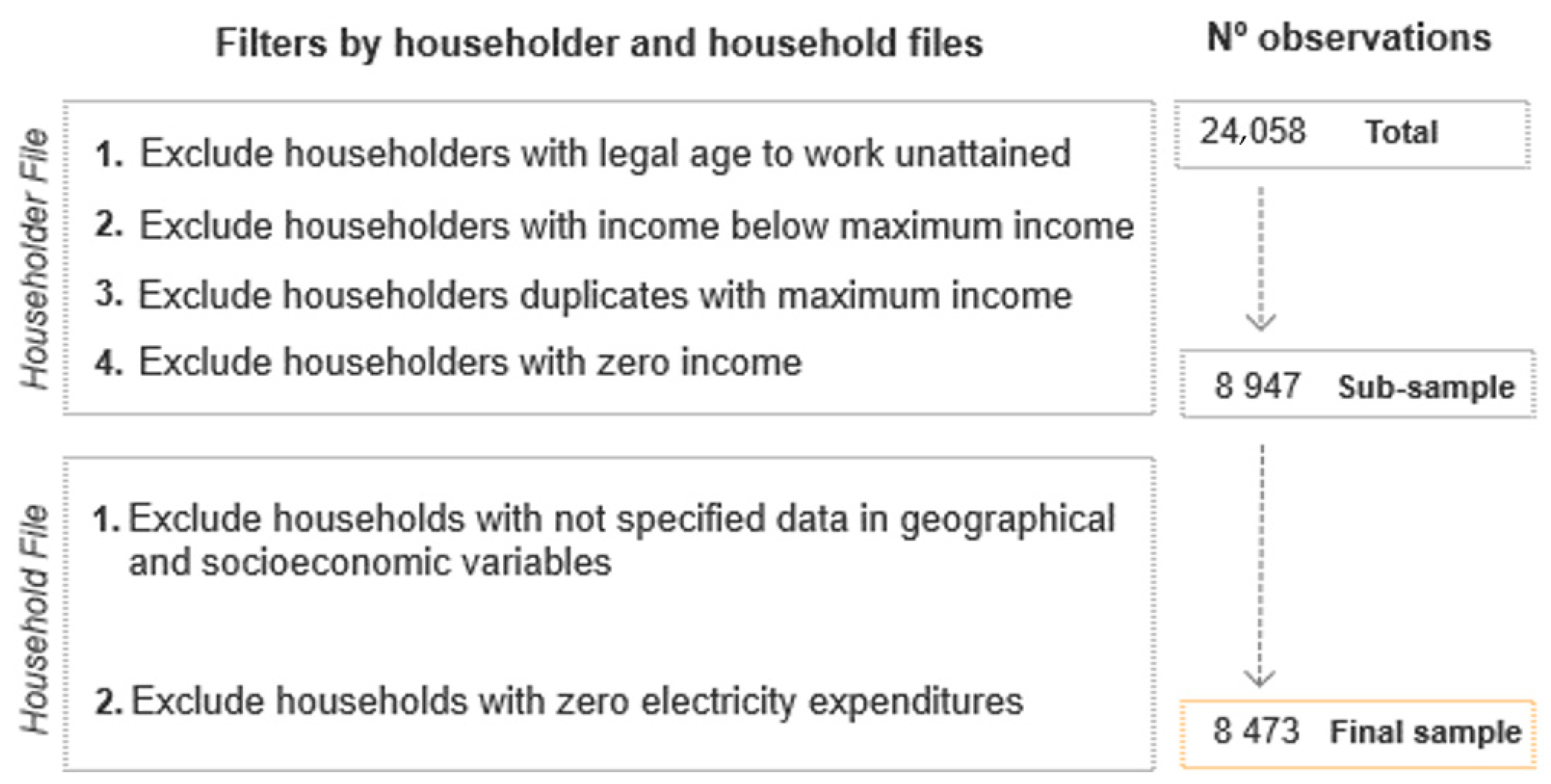
This information is organized into Household and the Household Members files. Within these files, information is grouped into basic variables at household level, which relate to identification, weighting and demographic characteristics of the households’ income and consumption expenditure data [46]. Similarly, basic variables at household member level account for: identification and weighting; gender, age, marital status, country of birth; education level, activity status and income [46]. The sample size for 2010 HBS edition included a total of N = 9489 household units and N = 24,383 householders in Portugal. This original sample underwent a filtering process, in order to promote a match between households as a whole and householders, based on the household reference person (HRP) concept as well as to exclude missing data. The exclusion criteria followed is illustrated in Figure 1.
From Figure 1, it is possible to see a substantial reduction in sample size, from an initial N = 24,383 observations to a sub-sample with N = 8947 observations, based on filtering steps 1–4. This size reduction is needed to establish a single person or householder (HRP) for each household. For Portugal, the reference person (HRP) corresponds to the person aged 16 or more and with the highest annual income, for a given family household [48,50]. Taking into consideration this definition filter (1) excludes all household members whose age is below to 16 years of age (legal age to work unattained). Based on the reference person concept, filter (2) excludes household members with incomes that do not correspond to the highest annual income for a given household or “income profile”. Conversely, in order to establish one single household member as reference person (HRP), filter (3) excludes duplicate household members with highest income. Filter (4) excludes households with zero income reported since it is not possible to establish the HRP concept, based on “income profile”. This way, the householder file becomes compatible with the household file, defining the sub-sample from the initial total number of observations. The advantage of the use of a single individual per household, such as in the HRP concept, is that it avoids subjective bias (see [51]) and avoids the difficulties of specific equivalence scales as described by the Organization for Economic Co-operation and Development (OECD) (2013) [52]. Together, filters for variables within householder file accounted for 15,436 dropped observations.
The final sample size (N = 8 473) has been established after excluding households for having reported zero cost for electricity expenditures. This filter was established given that access to residential electricity supply has 100% coverage at national level. According to the World Bank’s Sustainable Energy for All (SE4ALL) database [53], a time series for the last ten years (2007–2017), showed that indicators for access to electricity were 100% for both rural and urban areas. This time series is relevant, because it includes the most recent wave of HBS available, in 2010, used in the current research. Inexistent electricity costs, geographical and socioeconomic variables, namely education level, activity status and hours worked variables, contributed to excluding 474 observations.
2.2. Dataset and Variables: Dependent and Independent Variables
For the current assessment, the data from HBS on a variety of health care and household energy expenditures, as well as sociodemographic variables were drawn. These variables are categorized according to the Classification of Individual Consumption by Purpose (COICOP). A list of the variables considered in this study, according to this classification, is described in Table 1. Each of these main categories can be further disaggregated into sub-categories for households that participated in the survey, such as detailed fuel costs (e.g., electricity and natural gas), hospital services or prescriptions for health costs.
Among the advantages and main reasons for the use of HBS data is the free access and it being a database used for health and energy issues in prior studies. It gathers in a single database highly disaggregated information on consumption expenditures, but also provides additional data regarding the household´s sociodemographic context. Additionally, the use of expenditures has been considered more reliable as a measure of household resources in prior studies concerning household health costs [54]. However, a drawback from resorting to this database is that health status, considered one of the influencing factors of health expenses [40], is not included. For the HRP, variables such as age, gender, birthplace, marital status, education level, income and employment status have also been defined to characterize the observed population. Each household geographic context (region of the country and population density) has been considered as well.
Income and energy expenditures are annualized, and similarly to prior studies for different countries [33,55,56], they have been organized into low, medium and high levels. Similarly, this organization of income into levels has been also adopted for Portugal by Gouveia et al. [6,57]. This study adapts this concept to establish yearly income levels. Segmentation of energy according to low medium and high consumption profiles has also been previously performed by [58,59]. Here, this concept has been adapted and applied to define energy cost profiles. The abovementioned studies are surveys conducted at household level, and given that HBS are also conducted directly on a sample of households, this approach was considered suitable for the dataset used. Dummy variables representing the ‘use’, or ‘no use’ were developed to code other commodities (e.g., bottled gas). A similar procedure was developed for health insurance and rental status.
Total health expenditures correspond to the sum of all household health expenditures categories featured in Table 1.
To briefly summarize, this study includes additional energy-related variables, such as electricity expenditures, relevant at household level, to complement variables traditionally featured in the estimation of healthcare such as demographic, socioeconomic, and health insurance [56,60], with the exception of health status.
2.3. Model Specification
The total health expenditures were modeled according to a two-part model, following a statistical model design proposed by Belotti et al. [61] and Deb et al. [62]. The prediction of mean dependent variable health expenditures (Y), given explanatory variables (X), depends on both parts of the model, and can be written as in Equation (1).
The main focus of Part 1 from the Equation (1) is to model the probability of the household having any health expenditures; in Part 2, the main concern is to predict health expenditures conditional on households having them. Both parts of Equation (1) are associated with several model choices.
The main modelling choices have been identified by Deb and Norton [40]. The first choice refers to Part 1 of Equation (1), between logit and probit options, to model the probability of zero vs. non-zero expenditures. The second and third choices are explained below and correspond to the GLM model family and link choices. Similar to prior studies [42,61,63], this study has opted for a logit alternative to model the probability of having expenditures greater than zero, as defined by Equation (2). This option was based on the qualities of simplicity and interpretability the logit model presents in comparison to probit alternative [64].
Equation (2) corresponds to a binary response model, that assumes the value of 1 if health expenditure is positive, and assumes the value 0 otherwise [63].
where X stands for the vector of the independent variables and α for the vector of the regression coefficients for Part 1 of the model.
The remaining choices refer to Part 2 of Equation (1): the choice of link function and distribution family of the generalized linear model (GLM) to model a positive (non-zero) outcome. Standardized specification tests were performed to determine final model specification, namely box cox test to understand the link or transformation for the dependent variable (Y). The obtained coefficient from this test is close to zero, and indicative of a log transformation link. In order to determine the distribution family, a modified Park test was computed following the steps of Norton and Deb [40]. With a coefficient on the expected value close to 2.0, a gamma distribution was selected. The gamma distribution flexibility in specifying shape and rate parameters provides a way to deal with issues such as skewness and kurtosis, as well as a range of positive values with outliers (number of individual high expenditures) [65]. Therefore, the GLM with Gamma log link model has been considered an increasingly popular option to model health costs, helping with mass zeros and non-zero skewed distributions [37,39].
Taking into consideration the specification tests, the Part 2 model description can be written with Equation (3).
where β stands for the vector of regression coefficients for Part 2 of the model. As previously mentioned, each observation follows an exponential type gamma distribution with a log link function; therefore, each coefficient β is interpreted as a percentage change, given by , as decribed by Norton et al. [66]. Based on Equations (2) and (3) from Kyriopoulos et al. [34], the final equation for the two-part model can re-written as presented in Equation (4).
Additionally, specification tests for independent variables such as Pregribon and Ramsey RESET tests were also conducted. This procedure has been applied previously by several authors (see [40,42,63]) to detect misspecification by omitted variables. Performed tests were non-significant, meaning that the model is well specified and does not need additional variables.
Moreover, in the result section, the use of Average Adjusted Predictions (AAP) is favored to convey two-part model results. Adjusted predictions and marginal effects are alternative ways to present the results from a modelling approach, making them easier to understand and interpret [67,68]. Their use enables us to visually understand differences across variables of interest, such as age, income or electricity expenditure, giving obtained results a “substantive and practical significance.”, as emphasized by Williams [67]. Stata commands ‘margins’, and ‘maginsplot’, developed by Williams, were used [69].
To determine the relative importance of energy-related variables in the statistical model, a dominance analysis (DA) was undertaken. In order to compute it, the general dominance equation for each independent variable x (i.e., Cx), suggested by Luchman (2015) [45], was adopted:
“where Fij is the fit metric associated with model ij, p is the number of independent variables in the model, ni stands for the number of possible combinations of size i given the p independent variables, and C(m,k) is the number of combinations of size k possible given set size m” [45] (p. 2). According to Azen and Traxel (2009), the importance is defined by pairwise comparison of predictors (i and j) from a selected model (model ij) across all subsets of predictors to establish relative importance or dominance, requiring for the effect only a measure of model fit, such as R2. Therefore, dominance analysis enables us to define “the additional contribution of any given predictor to a given subset model as the change in R2 when the predictor is added to the model” [70] (p. 324). Dominance analysis was performed using Stata software, resorting to the ‘domin’ command [71].
Prior to the statistical analysis, a brief summary statistic of the sample is provided in the next section.
2.4. Sample Summary Statistics
Table 2 presents the summary statistics for the final sample, according to their groupings: geographic, socioeconomic, and energy expenditure. A few aspects regarding the sampled population are emphasized here. Regarding demographic characteristics, there is a prevalence in the sample of mainland households (81.53%) in comparison to Madeira and Azores. These household units seem to be located in sparsely populated areas (63.21%). About 60% of the population is male in gender, from older age ranges and lower education levels. Just over 90% of the population is national, working and to a large extent belongs to the medium income level. Household composition varies greatly, with greater presence of adults without children, of different age ranges but with high share of elderly population. Household composition and size (n° of people according to each age range) follow the harmonized categories that classify household members into adults and children, according to Eurostat’s HBS methodology [46,49].
Most householders working fulltime are homeowners and without private health insurance, as the National Health Service provides coverage to all population. Most households have a medium electricity expenditure, where bottled gas expenses seem to prevail over natural gas ones, with low use of liquid and solid fuels.
3. Results
In this section the results from the statistical analysis conducted are provided. The outcome from the two-part model is presented to establish the associations between overall health expenditures, energy expenditures and sociodemographic variables. For significant associations, results are also reported as Average Adjusted Predictions (AAP) to provide a better understanding of the amount of the model coefficients and the change in health expenditures produced by one unit change in the independent variable or in comparison to the reference level, depending on if the variable is continuous or categorical in nature.
Second, results from the conducted dominance analysis are presented to understand the explanatory power of independent variables. A rank of the relative importance of different independent variables included in the model is provided.
3.1. Main Findings
The focus of this section is to present two-part model results. Parameter or coefficient estimates from the regression model are presented in Table 3. These coefficients reflect the association or effect that independent variables have on healthcare expenditures. The logit model (part 1) indicates the likelihood of having any expenditure versus not having them. Meanwhile, the GLM model (part 2) indicates the increase or decrease in spending, conditional on having any expenditure.
According to Table 3, several model coefficients show different signs and levels of significance, for each part of the model. These coefficients are reflective of the relationship between the dependent and independent variables. The coefficients for the logit model (part 1) are in log-odd units, and depending on their sign, allow to infer whether having health expenditures is a more likely (log-odds > 0) or less likely (log-odds < 0) event. In the GLM model (part 2) with a log link function, variable coefficient can be interpreted as a percentage change regarding the reference level. The overall predicted health expenditure is obtained from the multiplication of the predictions from the logit model (part 1) and the GLM model (part 2), as shown in Equation (1). As a result, the two-part model combined estimates may not all be jointly significant. Yet, these variables may be significant for each part of the model separately.
As illustrated in Table 3, there are highly significant explanatory variables for having health expenditures, among all the categories featured in the model, i.e., geographic, socioeconomic and energy expenditure. However, given that the main focus of the current study is to better understand the role of energy expenditures as an explanatory variable for health, other significant explanatory variables are focused on, taking into consideration their relationship with energy and particularly with electricity expenditures. The use of adjusted predictions and marginal effects is required to graphically illustrate how health expenditures change according to age range or income level and electricity expenditure, within the energy expenditure category. Average adjusted predictions (AAPs) are used to visually translate the association between the dependent variable and a given independent variable as the predicted estimate, while all other variables are left at their observed values [72]. They are used to improve the perception of the outcome of the two-part model, since the coefficients in both parts of the model are difficult to interpret, based only on the sign and statistical significance.
According to Table 3, electricity expenditures stand out among the energy category, as it is the only energy alternative that is statistically significant for part 1 and part 2 of the two-part model. Overall, electricity presents a positive coefficient for both the logit and GLM model. This entails that the probability of having health expenditures and its amount increase with electricity expenditures. Overall, the electricity expenditure variable is associated with an increased probability of having health expenditures (by 9.75%), according to Equation (2), for the logit model (part 1). With a higher level of significance (p < 0.001), the amount of health expenditures increases by 8.00% (0.080= (e0.078)) − 1)), from Equation (3), for the GLM model (part 2). Further analysis is conducted in the next section.
3.2. Discussion
The main results from the two-part model are further discussed. The critical analysis takes into consideration significant variables of interest, such as age, income and electricity expenditures. This critical analysis is followed by a dominance analysis (DA).
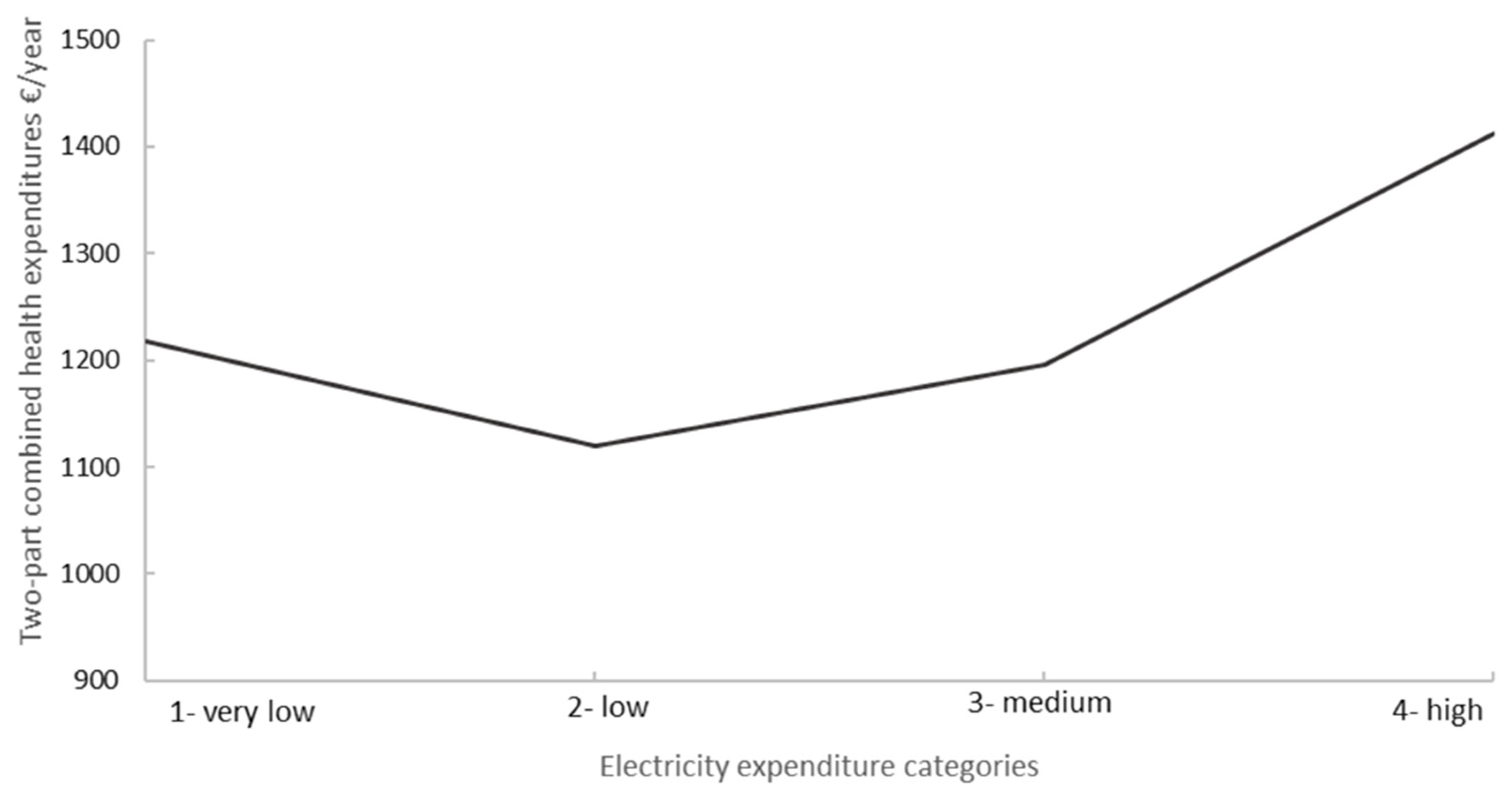
In Figure 2, a more detailed look at the two-part model’s health expenditure for all electricity expenditure categories is displayed. For each category of electricity expenditures, variation among different levels is revealed. For instance, higher health expenditures are expected for very low electricity expenditure level in comparison to low and medium electricity expenditure levels. Moreover, other socioeconomic variables are taken into consideration to contextualize obtained results.
According to Table 3, it is also possible to see that other energy variables, particularly for liquid and solid fuels, present higher positive and significant coefficients, only for the logit model (part 1). Liquid fuels include domestic heating and lighting oil, which similarly to solid fuels might be more carbon intensive energy alternatives. Their use and exposure might imply higher probability of incurring health expenditures. This argument is plausible, as prior studies have emphasized the adverse health implications of the use of carbon intensive fuels, though mostly related to developing countries [72,73].
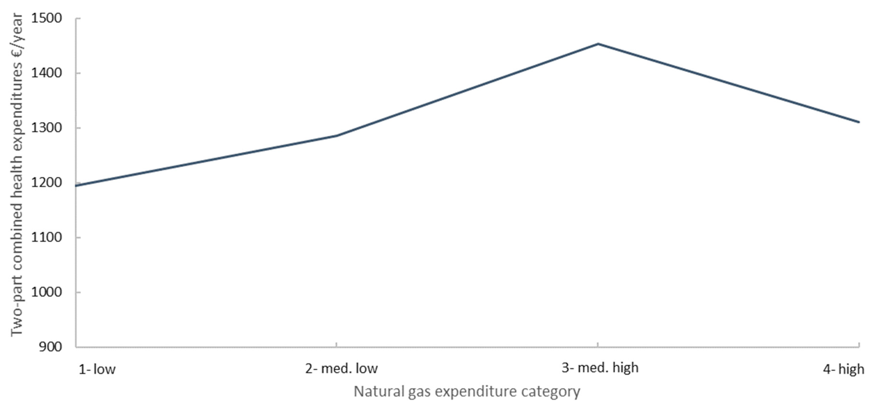
The stronger contribution of logit model (part 1) in comparison to GLM model (part 2) for two-part combined estimate for health expenditure is also noticeable for natural and bottled gas (both with higher positive and significant coefficients). According to Figure 3, health expenditures tend to increase with increasing levels of natural gas expenditure (from level 1 to level 3) and then suffer an abrupt decrease at higher levels of expenditure (from level 3 to level 4). The estimated overall health expenditures reaches about 1450 €/year for people included in level 3 and drops about 150 € in comparison to the reference level (level 1), as illustrated in Figure 3.
In fact, Figure 3 shows that the reduction from level 3 to level 4 is outweighed by the increase from level 2 to level 3, which is consistent with small and non-significant GLM coefficient in Table 2. A possible explanation should take into consideration summary statistics of the dataset, presented in Table 2. According to Table 2, high natural gas expenditures represent a very small share of sampled households (1.56%), in comparison to other levels, such as low natural gas expenditures (84.70%). This share corresponds to a total of N = 132 units in a universe of N = 8 473 households. Therefore, any conclusions for the high natural gas expenditure segment may be difficult to justify.
The prevalence of lower natural gas expenditure levels could also be related to the location of the households, mostly in sparsely populated areas (rural areas), as illustrated in Table 2. In Portugal, natural gas connection is typical for urban, densely populated areas, with a lower share in the analyzed sample (29.87%). This information from summary statistics might help contextualize and interpret the obtained results. Yet, as previously mentioned, statistical inferences are premature, given the nature and size of the sample for the case of gas. Two-part combined health expenditures are estimated to be higher for people who use bottled gas (1230 €/year) than for people that do not use it (1180 €/year). Conversely to natural gas, bottled gas is a common energy alternative for sampled households, supplying over 70% of households. This corresponds to about N = 5 947 in comparison to natural gas and is in accordance with the rural setting. The difference of close to 50 €/year for health expenditures occurs when there is a change from 0 (no use) to 1 (use). Similarly, for natural gas, this increase is spurred by part 1 of the model given the small and non-significant value for the GLM coefficient.
For age-related variables, such as age range and the number of people above a given age range, the results from the logit model (part 1) indicate that, ceteris paribus, the likelihood of having health expenditures increases by 0.112 or 10.01% in comparison to the reference category. The results for the GLM model (part 2) show that the model coefficient is positive, in alignment with the logit model (part 1). Therefore, in comparison to the reference category (15–29) (15 to 29 years old) there is a 10.2% (from Equation (3) increase in the health expenditures, when they exist. As the number of people between 25 and 65 years old included in the household composition increases, so does the likelihood of having increased health expenditures. This likelihood increases by 0.264 in comparison to the reference level. The reference level is defined by Stata software as the less frequent category (zero people between 25 and 65 years old). Therefore, in households with people between 25 and 65 years old, there is an increased probability of 20.89% of having additional health expenditures in comparison to households without any people between 25 and 65 years old.
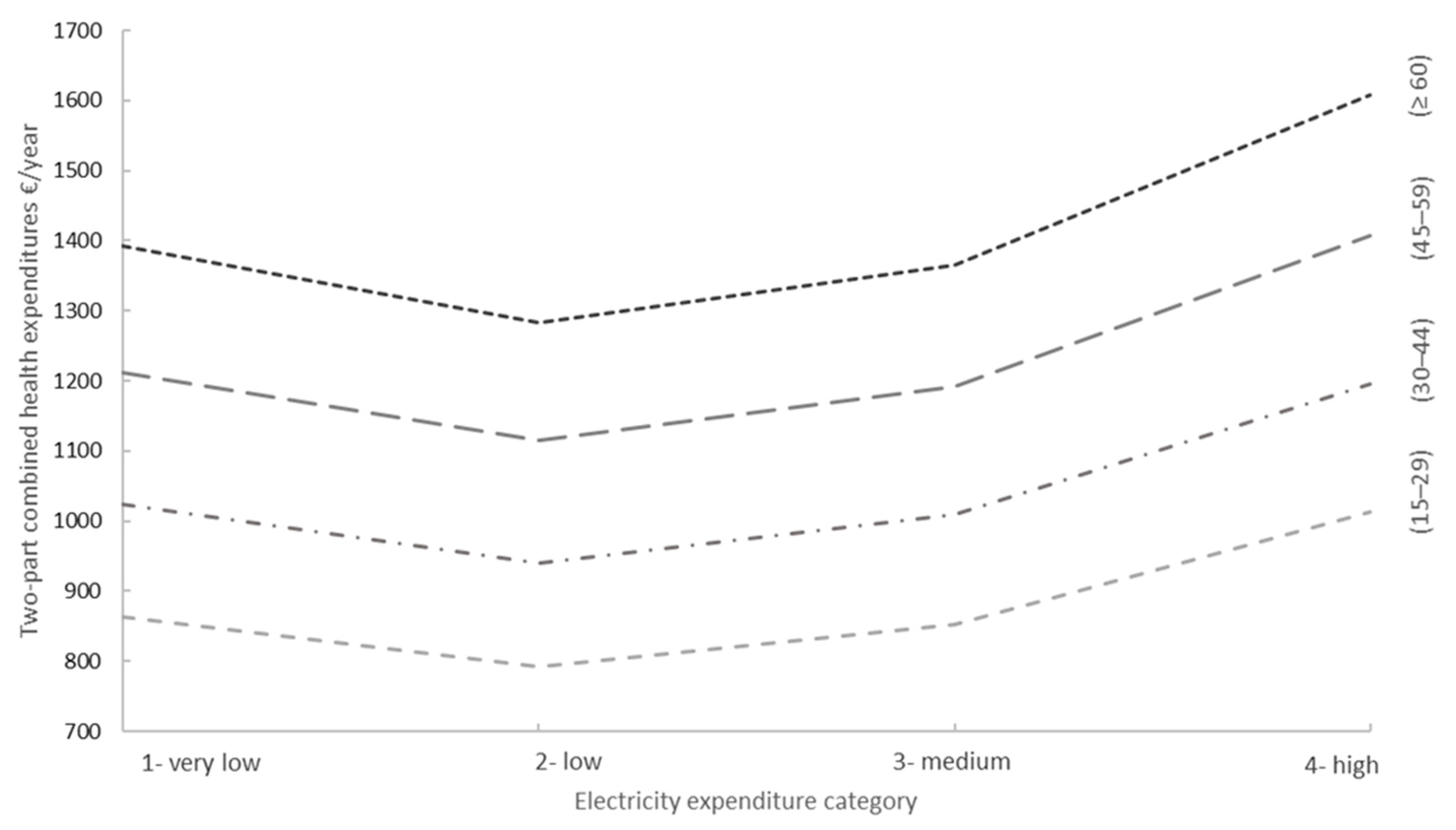
Similarly, for each additional person above 65 in the household composition, the predicted log odds are expected to increase by 0.556, in comparison to no people above 65 (reference level) or 35.73%. Therefore, a greater likelihood of having health expenditures is expected for higher levels of the coefficient. The changes in health expenditure by electricity expenditure and age range are presented in Figure 4.
In Figure 4, average adjusted predictions (AAP) for electricity expenditure by each age range shows the incremental effect of age. In comparison to people of lower age ranges, people over 60 (≥60) are associated with higher electricity expenditures and higher health expenditures. For instance, for the low (2) electricity expenditure category, the estimated overall health expenditure is 800 €/year for people between 15 and 29 (15–29) and increases to over 1200 €/year for people over 60 (≥60). These results are plausible since, as one of the most vulnerable segments of the population, the elderly tend to incur increased health expenditures. Also, given their need to keep warm at home, they have been known to increase energy expenditures [74,75].
The analysis of all age groups presents higher health expenditures than the reference age level (15–20) (15–29 years old). People over 60 (≥60) from low and medium electricity expenditure categories experience a decrease in health expenditure, in comparison to very low electricity expenditure, as illustrated in Figure 4. Low and medium electricity expenditure categories experience a decrease in health expenditure, in comparison to very low electricity expenditure, across all age ranges. However, this difference is particularly remarkable for people over 60 (≥60) years old for who the difference in health expenditures to reference level amounts to −110 €/year. It should also be noticed in Figure 4, that people over 60 (≥60) with very low electricity expenditure are estimated to have heath expenditures almost as high as the highest electricity expenditure groups (1400 €/year for the former versus 1600 €/year for the latter).
A similar interpretation is required for the increasing number of people above 65 living in the same house, i.e., they tend to increase health expenditures. Although for each electricity expenditure category, the higher number of people above 65 tends to lead to a higher health expenditure in Figure 5, low and medium electricity expenditure categories tend to have lower health expenditures in comparison to very low electricity expenditure.
In Figure 5, households with one household member over 65 years of age seem to have health expenditures close to the ones with two or more household members over 65 years. The decreasing impact of one additional household member in electricity expenditures has been reported in previous studies [55]. These results are aligned with recent European Union trends, that claim that a growing share of older people live alone, i.e., in households composed of a single person, particularly older women [76]. Further information regarding health status and living conditions is required to draw any conclusions regarding this result. Yet, even taking into consideration the increasing effect of age-related variables, these results are aligned with prior trends for electricity, in Figure 2.
Moreover, the relationship between other significant variables for health expenditures should also be considered to establish whether this result of (very) low electricity-high health expenditures takes place in a low-income context, possibly affecting vulnerable segments of the population. Low electricity-high health expenditure within a low-income context could configure a situation of energy insecurity/poverty at household level. In southern European countries, Castaño-Rosa et al. (2020) claim that people in cold and energy inefficient households run the risk of developing cold-related diseases while struggling to meet their energy needs [77]. Among the health impacts in household communities, energy insecurity has been identified as being significantly associated with poor respiratory, mental health, and sleep outcomes by Hernandez and Siegel (2019) [78]. This risk could lead to an increased need for healthcare services, which could contribute to increasing household health expenditure burden, that is aligned with the obtained low electricity-high health expenditure situation. Furthermore, despite the warm weather, Portugal has been repeatedly considered one of the countries most affected by this issue [3,79].
Income is also amongst the statistically significant variables for both parts of the model. Overall, according to Table 3, the likelihood of having health expenditures is increased by 0.119, in the logit model (part 1). This means that in comparison to the reference level (low income) there is an increased probability to incur in health expenditures by 10.63%. This result is significant at 5% level. The greater impact of this explanatory variable is felt in the GLM model (part 2), with a higher coefficient and significance level. Conditional on having health expenditures, the amount of health expenditures increases by 19.48% (exp (0.1948 = ( in comparison to low-income level. This result is statistically significant at 1% level.
Obtained results regarding the relationship between health expenditures-income-age and electricity expenditures are illustrated in Figure 6. As expected, health expenditures increase according to age and income level. This is visible for the adjusted prediction values in Figure 6. These results are in accordance with prior results for age-related variables.
As for the relationship between health, income and electricity expenditures, the Figures show that at each income level the category of very low (1) electricity expenditures presents higher health expenditures than low (2) electricity expenditures and at the same level of medium (3) electricity expenditures. For instance, at the low-income level, the value of health expenditures decreases by 70 €/year for low electricity expenditure in comparison to very low electricity expenditure (reference level).
This is a transversal pattern, across all income levels. It shows that regardless of the income level, the lowest electricity expenditure category tends to have higher health expenditures than the following category, as illustrated in Figure 7. These results point to the existence of a relationship that may be described as a (very) low electricity expenditure-high health expenditure situation across all income levels. The identified U-trend for health expenditures would be consistent with householders, particularly elderly, who are more likely to spend more time in hospital or day-care centers than in their home, decreasing their electricity expenditures and increasing health expenditures. Thus, this emphasizes the relevance of these expenditures in relation to income and age and the need to further investigate them. These results for (very) low electricity expenditures could imply differences from an energy efficiency perspective that require further research related to the household building characteristics for all income levels, which are not available in the database. However, this is particularly relevant for the vulnerable segments of the population, with low-income levels, since it configures the previously identified possibility of household energy poverty. According to Mohan (2021), despite this issue being recognized as a concern, its impacts are still understudied for vulnerable segments of the population [80].
These results draw the attention of policy makers to an issue that could easily be overlooked, given the lower share of low-income and very low electricity expenditure households in the sample. It also allows them to target this vulnerable group as a priority candidate for efficiency improvements at household level. Efficiency improvements at envelope level, such as wall insulation, and change to energy efficient doors and windows have been known to improve indoor temperatures [81]. Cold homes associated with low energy efficiency have been identified as one of the causes of the inability to conciliate indoor comfort with increasing energy expenditures (see [75]). Therefore, based on obtained results, this work somewhat supports the view that investment in energy efficiency could contribute to reducing both energy and health expenditures for vulnerable populations, such as low-income elderly households.
Furthermore, given the high differentiation of results by income, age and electricity-expenditure categories and their statistical significance, it is plausible that the trends identified for vulnerable households could be used as a steppingstone to further explore housing conditions to address electricity and health expenditures. This information on the relationship between income, age, electricity and health, provided in this study, could then be crucial to identify and target priority action groups for the future development of policies at local community level, taking into consideration the insight from energy and health stakeholders.
This inclusive and multidisciplinary approach, suggested by obtained results, supports Kahouli’s (2020) idea that, in the context of energy poverty, housing energy efficiency measures might constitute a solution to promote the reduction of public health care expenditure in the long term [51]. “Local action” has been considered by Bergman and Foxon (2020) as a potential aspect/driver for reframing housing energy efficiency policies, by engaging and promoting local authorities or local and regional partnerships [82]. Meanwhile, according to Mallabanda and Lipson (2020), health and thermal comfort have been identified within a range of householder needs that low carbon energy policies should meet in order to be successful [83]. In fact, a recent study by Ahn (2021) has emphasized the relevance of developing new modelling approaches to improve efficiency of energy use that determine thermal quality of the space [84]. These results are also reinforced by the study of Pais-Magalhães et al. (2020), that emphasized the challenges electricity consumption at household level faces with the aging population, requiring the development of energy efficiency policies that take into consideration the needs of the elderly [85].
A dominance analysis (DA) is also used to determine the order or rank of energy expenditure as an explanatory variable for health expenditure. It allows us to establish the relative importance, from most relevant to least relevant, or explanatory power of independent variables considered. According to the results and for those with health expenditures, electricity expenditure has been disclosed as a relevant explanatory variable for the value of the health expenditures, though it has often been neglected in this context. It is ranked in fifth place out of 26 explanatory variables included in the two-part model. Also, in the top 5 rank, electricity expenditures are preceded by income, the number of people above 65, the age range and education level, as presented in Table 4. These values are based on changes in R2, and the dominance standardized estimates represent the ”proportion of each factor’s explained variance of the variance explained by the whole model” [86]; in this particular case, DA was applied for those who present health expenditures. Therefore, it is not expected to be reflective of the entire model but gives an idea of the relative importance of independent variables of interest in explaining the variance in the dependent variable. For instance, based on Table 4, electricity expenditures played a relevant role in DA, explaining 6.71% of the variance of health expenditure.
This DA further emphasizes the need to consider energy-related variables as explanatory variables for health issues. Despite this, although all top ranked explanatory variables show high statistical significance (1% level), this ranking presents some differences regarding the coefficients from the two-part model; this is because the coefficients are not directly comparable, as different scales are used for each variable. Dominance analysis also reinforced the connections explored between different explanatory variables. The relationship between energy, age, income and health is also in accordance with other emerging concepts such as aging in place, and healthy aging that contribute towards a more efficient, greener and age-friendly city.
4. Conclusions and Future Research
Overall, the aim of the present study, using the two-part model and microdata from Eurostat Household Budget Survey (HBS), was to investigate the association between energy and health expenditures and determine the role of electricity expenditures as an explanatory variable for health expenditures.
Our findings suggest that given the high significance and coefficient value, electricity expenditure is a relevant explanatory variable for health expenditures. This result is further validated by the top 5 position in the dominance analysis ranking. The assessment with other explanatory variables of interest, such as income and age-related variables, enabled us to identify vulnerable target groups, and could act as triggers for further research in unison with housing and health conditions at the basis for the development of policies, with the aim of reducing health expenditures through the reduction of energy expenditures.
This study contributes to demonstrating the existence of a relationship that can be described as (very) low energy expenditure-high health expenditure, in Portugal. This might be a pattern across all income levels; nonetheless, obtained results call the attention of policy makers to the low-income-(very) low energy expenditure-high health expenditure relationship that could configure a household energy poverty situation. The (very) low energy expenditure-high health expenditure trend, common to all income levels, also enables some considerations as to how energy efficiency could be experienced across several segments of the population. In this particular case, the evidence suggests that, regardless of the income level, for households with very low energy expenditures, energy efficiency benefits could be experienced differently. In households with very low electricity expenditures, in the case of energy efficiency measures, spending could be further reduced although in limited extension. However, it is expected that these energy efficiency measures could have a major impact in bettering living conditions, namely adequate indoor temperature. Therefore, the development of energy efficiency policies should contribute to improving indoor temperature without necessarily increasing energy expenditures. Especially for the abovementioned vulnerable segment of the population, these policies should then focus on the improvement of living conditions and by this enabling the decreasing of health expenditures. Meanwhile, for higher income segments, the development of energy efficiency policies could be translated into both energy expenditure savings and higher indoor temperature, potentially also leading to a health co-benefit, and a reduction in health expenditures.
The translation of energy efficiency into health co-benefits requires additional information on building characteristics and health status. These findings support the need to assess investment in improving housing conditions under a social cost-benefit analysis. Recent studies consider new policy framings such as new business models to incorporate health and wellbeing into housing energy efficiency policies [82,87]. Meanwhile, Ezratty et al. (2018) have proposed a methodology to assess the health cost implications of fuel poverty [88]. The evaluation of the economic interest of energy efficiency projects must then go beyond the traditional estimation of energy cost reduction and must recognize also likely health gains and avoided medical costs. Therefore, in this sense, housing energy efficiency measures could improve and encourage the development of efficient public health policies regarding health expenditures, based on the assessment of energy efficiency’s health gains and avoided medical costs.
The present study provides key information regarding the relevance of energy-related and health expenditures, that could be of use for vulnerable households that suffer added pressure in the context of climate change. However, a deeper understanding between housing conditions and their interaction with health status, such as chronic conditions under a changing climate, is required. Thus, obtained results also call attention of policy makers towards the need to take into consideration not only economic and environmental impacts but also health impacts in future design of energy efficiency policies. The implementation of energy efficiency measures that take into consideration the interaction between energy, other explanatory variables and health could contribute towards climate change targets by reducing energy expenditures while protecting health from inadequate heat or cold exposure. Other emerging concepts such as “ageing in place”, that ultimately contribute towards accomplishment of energy and health-related SDGs, could also be simultaneously promoted.
Yet, it is recognized that results from the current research are hindered by the nature of the data available at the HBS dataset, since they lack specific information regarding health (e.g., health outcomes) and energy efficiency (e.g., level of thermal insulation) and appliances (e.g., heating and cooling systems ownership). Further efforts should, therefore, focus on the inclusion of building and health status information, to understand and promote how living conditions influence health and how to develop synergies with building energy efficiency strategies.
Author Contributions
Conceptualization, F.L. and P.F. and V.L.; methodology, F.L.; software, F.L.; supervision, P.F. and V.L.; validation, P.F. and V.L. formal analysis, F.L. and P.F. and V.L.; investigation, F.L. and P.F. and V.L.; resources F.L. and P.F. and V.L.; data curation, F.L. and V.L.; writing—original draft preparation, F.L.; writing—review and editing, P.F. and V.L. All authors have read and agreed to the published version of the manuscript.
Funding
This research was funded by FCT–Fundação para a Ciência e Tecnologia within MIT SES Portugal Doctoral Program under the scholarship PD/BD/128029/2016. This work has also been supported by FCT–Fundação para a Ciência e Tecnologia within the R&D Units Project Scope: UIDB/00319/2020.
Institutional Review Board Statement
Not applicable.
Informed Consent Statement
Not applicable.
Data Availability Statement
3rd Party Data Restrictions apply to the availability of data used and the STATA model developed. Data was obtained from Eurostat HBS database (https://ec.europa.eu/eurostat/web/microdata/overview), accessed on 23 October 2019. A confidentiality agreement was signed and the data cannot be publicly disclosed.
Acknowledgments
The researchers further like to acknowledge the financial support by FCT–Fundação para a Ciência e Tecnologia within MIT SES Portugal Doctoral Program under the scholarship PD/BD/128029/2016. This work has also been supported by FCT–Fundação para a Ciência e Tecnologia within the R&D Units Project Scope: UIDB/00319/2020. For the analysis, the authors used data from the HBS, which are available upon request at https://ec.europa.eu/eurostat/web/microdata/overview, accessed on 23 October 2019. The authors are thankful for the authorization granted. The responsibility for all conclusions drawn from the data lies entirely with the authors.
Conflicts of Interest
The authors declare no conflict of interest.
Nomenclature
| AAP | Average adjusted predictions |
| COICOP | Classification of Individual Consumption by Purpose |
| DA | Dominance Analysis |
| EU | European Union |
| GLM | Generalized linear model |
| HBS | Household Budget Survey database |
| HRP | household reference person |
| INE | Statistics of Portugal |
| LPG | Liquefied Petroleum Gas |
| OECD | Organisation for Economic Co-operation and Development |
| OLS | Ordinary least squares |
| OR | Odds ratio |
| SE4ALL | Sustainable Energy for All database |
| UK | United Kingdom |
| WHO | World Health Organization |
References
- Pyrgou, A.; Castaldo, V.L.; Pisello, A.L.; Cotana, F.; Santamouris, M. On the effect of summer heatwaves and urban overheating on building thermal-energy performance in central Italy. Sustain. Cities Soc. 2017, 28, 187–200. [Google Scholar] [CrossRef]
- Daniel, L.; Baker, E.; Williamson, T. Cold housing in mild-climate countries: A study of indoor environmental quality and comfort preferences in homes, Adelaide, Australia. Build. Environ. 2019, 151, 207–218. [Google Scholar] [CrossRef]
- Guertler, P.; Smith, P. Cold Homes and Excess Winter Deaths a Preventable Public Health Epidemic That Can No Longer be Tolerated; E3G: London, UK, 2018. [Google Scholar]
- Taylor, J.; Symonds, P.; Mavrogianni, A.; Davies, M.; Shrubsole, C.; Hamilton, I.; Chalabi, Z. Modelling population exposure to high indoor temperatures under changing climates, housing conditions, and urban environments in England. In Proceedings of the 2016 International Conference on Urban Risks (ICUR 2016), Boise, ID, USA, 27–28 September 2016; pp. 1–8. [Google Scholar]
- McDowell, C.; Kokogianakis, G.; Gomis, L.L.; Cooper, P. Relationship Between Indoor Air Temperatures and Energy Bills for Low Income Homes in Australia. Energy Procedia 2017, 121, 174–181. [Google Scholar] [CrossRef]
- Gouveia, J.P.; Seixas, J.; Long, G. Mining households’ energy data to disclose fuel poverty: Lessons for Southern Europe. J. Clean. Prod. 2018, 178, 534–550. [Google Scholar] [CrossRef]
- Howden-Chapman, P.; Roebbel, N.; Chisholm, E. Setting Housing Standards to Improve Global Health. Int. J. Environ. Res. Public Health 2017, 14, 1542. [Google Scholar] [CrossRef] [PubMed] [Green Version]
- Morey, J.; Beizaee, A.; Wright, A. An investigation into overheating in social housing dwellings in central England. Build. Environ. 2020, 176, 106814. [Google Scholar] [CrossRef]
- Pathan, A.; Mavrogianni, A.; Summerfield, A.; Oreszczyn, T.; Davies, M. Monitoring summer indoor overheating in the London housing stock. Energy Build. 2017, 141, 361–378. [Google Scholar] [CrossRef]
- Santamouris, M. Recent progress on urban overheating and heat island research. Integrated assessment of the energy, environmental, vulnerability and health impact. Synergies with the global climate change. Energy Build. 2020, 207. [Google Scholar] [CrossRef]
- World Health Organization. WHO Housing and Health Guidelines; World Health Organization: Geneva, Switzerland, 2018. [Google Scholar]
- John, A.; Hermelink, A.; Galiotto, N.; Foldbjerg, P.; Eriksen, K.B.M.; Christoffersen, J. Study shows that unhealthy homes lead to reduced health. REHVA J. 2018, 3, 19–22. [Google Scholar]
- Boch, S.J.; Taylor, D.M.; Danielson, M.L.; Chisolm, D.J.; Kelleher, K.J. Home is where the health is: Housing quality and adult health outcomes in the Survey of Income and Program Participation. Prev. Med. 2020, 132, 105990. [Google Scholar] [CrossRef]
- Novoa, A.M.; Ward, J.; Malmusi, D.; Díaz, F.; Darnell, M.; Trilla, C.; Bosch, J.; Borrell, C. How substandard dwellings and housing affordability problems are associated with poor health in a vulnerable population during the economic recession of the late 2000s. Int. J. Equity Health 2015, 14, 1–11. [Google Scholar] [CrossRef] [PubMed] [Green Version]
- Tabata, T.; Tsai, P. Fuel poverty in Summer: An empirical analysis using microdata for Japan. Sci. Total Environ. 2020, 703, 135038. [Google Scholar] [CrossRef]
- Memmott, T.; Carley, S.; Graff, M.; Konisky, D.M. Sociodemographic disparities in energy insecurity among low-income households before and during the COVID-19 pandemic. Nat. Energy 2021, 6, 186–193. [Google Scholar] [CrossRef]
- Willand, N.; Ridley, I.; Maller, C. Towards explaining the health impacts of residential energy efficiency interventions—A realist review. Part 1: Pathways. Soc. Sci. Med. 2015, 133, 191–201. [Google Scholar] [CrossRef]
- Gibson, M.; Petticrew, M.; Bambra, C.; Sowden, A.J.; Wright, K.E.; Whitehead, M. Housing and health inequalities: A synthesis of systematic reviews of interventions aimed at different pathways linking housing and health. Health Place 2011, 17, 175–184. [Google Scholar] [CrossRef] [Green Version]
- Fisk, W.J.; Singer, B.C.; Chan, W.R. Association of residential energy efficiency retrofits with indoor environmental quality, comfort, and health: A review of empirical data. Build. Environ. 2020, 180, 107067. [Google Scholar] [CrossRef]
- Gilbertson, J.; Grimsley, M.; Green, G. Psychosocial routes from housing investment to health: Evidence from England’s home energy efficiency scheme. Energy Policy 2012, 49, 122–133. [Google Scholar] [CrossRef]
- Poortinga, W.; Jones, N.; Lannon, S.; Jenkins, H. Social and health outcomes following upgrades to a national housing standard: A multilevel analysis of a five-wave repeated cross-sectional survey. BMC Public Health 2017, 17, 927. [Google Scholar] [CrossRef] [PubMed] [Green Version]
- Redvers, N. The determinants of planetary health. Lancet Planet. Health 2021, 5, e111–e112. [Google Scholar] [CrossRef]
- MacNeill, A.J.; McGain, F.; Sherman, J.D. Planetary health care: A framework for sustainable health systems. Lancet Planet. Health 2021, 5, e66–e68. [Google Scholar] [CrossRef]
- Vardoulakis, S.; Dimitroulopoulou, C.; Thornes, J.; Lai, K.-M.; Taylor, J.; Myers, I.; Heaviside, C.; Mavrogianni, A.; Shrubsole, C.; Chalabi, Z.; et al. Impact of climate change on the domestic indoor environment and associated health risks in the UK. Environ. Int. 2015, 85, 299–313. [Google Scholar] [CrossRef] [Green Version]
- World Health Organization. Healthy Ageing and the Sustainable Development Goals; World Health Organization: Geneva, Switzerland, 2020. [Google Scholar]
- World Health Organization. Non-Communicable Diseases and Their Risk Factors-Synergies for Beating NCDs and Promoting Mental Health and Well-Being; World Health Organization: Geneva, Switzerland, 2020. [Google Scholar]
- Nugent, R.; Bertram, M.Y.; Jan, S.; Niessen, L.; Sassi, F.; Jamison, D.T.; Pier, E.G.; Beaglehole, R. Investing in non-communicable disease prevention and management to advance the Sustainable Development Goals. Lancet 2018, 391, 2029–2035. [Google Scholar] [CrossRef]
- Tweed, C.; Dixon, D.; Hinton, E.; Bickerstaff, K. Thermal comfort practices in the home and their impact on energy consumption. Arch. Eng. Design Manag. 2013, 10, 1–24. [Google Scholar] [CrossRef]
- Ahn, M. Introduction to special issue: Aging in place. Hous. Soc. 2017, 44, 1–3. [Google Scholar] [CrossRef] [Green Version]
- Marshall, K.; Hale, D. Aging in Place. Home Health Now 2020, 38, 163–164. [Google Scholar] [CrossRef] [PubMed]
- van Hoof, J.; Schellen, L.; Soebarto, V.; Wong, J.; Kazak, J. Ten questions concerning thermal comfort and ageing. Build. Environ. 2017, 120, 123–133. [Google Scholar] [CrossRef]
- Salari, M.; Javid, R.J. Modeling household energy expenditure in the United States. Renew. Sustain. Energy Rev. 2017, 69, 822–832. [Google Scholar] [CrossRef]
- Besagni, G.; Borgarello, M. The determinants of residential energy expenditure in Italy. Energy 2018, 165, 369–386. [Google Scholar] [CrossRef]
- Besagni, G.; Borgarello, M. What are the odds? On the determinants of high residential energy expenditure. Energy Built Environ. 2020, 1, 288–295. [Google Scholar] [CrossRef]
- Wiesmann, D.; Azevedo, I.L.; Ferrão, P.; Fernández, J.E. Residential electricity consumption in Portugal: Findings from top-down and bottom-up models. Energy Policy 2011, 39, 2772–2779. [Google Scholar] [CrossRef]
- Matsaganis, M.; Mitrakos, T.; Tsakloglou, P. Modelling health expenditure at the household level in Greece. Eur. J. Health Econ. 2008, 10, 329–336. [Google Scholar] [CrossRef]
- Montez-Rath, M.; Christiansen, C.L.; Ettner, S.L.; Loveland, S.; Rosen, A.K. Performance of statistical models to predict mental health and substance abuse cost. BMC Med. Res. Methodol. 2006, 6, 53. [Google Scholar] [CrossRef] [PubMed] [Green Version]
- Shi, J.; Wang, Y.; Cheng, W.; Shao, H.; Shi, L. Direct health care costs associated with obesity in Chinese population in 2011. J. Diabetes Complicat. 2017, 31, 523–528. [Google Scholar] [CrossRef]
- Harrington, R.L.; Qato, D.M.; Antoon, J.W.; Caskey, R.N.; Schumock, G.T.; Lee, T.A. Impact of multimorbidity subgroups on the health care use of early pediatric cancer survivors. Cancer 2019, 126, 649–658. [Google Scholar] [CrossRef]
- Deb, P.; Norton, E.C. Modeling Health Care Expenditures and Use. Annu. Rev. Public Health 2018, 39, 489–505. [Google Scholar] [CrossRef] [PubMed] [Green Version]
- Veiga, P.A. Out-of-pocket health care expenditures due to excess of body weight in Portugal. Econ. Hum. Biol. 2008, 6, 127–142. [Google Scholar] [CrossRef] [PubMed]
- Tarazona, V.C.; Olmeda, N.G.; Consuelo, D.V. Predicting healthcare expenditure by multimorbidity groups. Health Policy 2019, 123, 427–434. [Google Scholar] [CrossRef]
- European Commission Eurostat. Household Budget Surveys (HBS)—Overview; Eurostat: Luxembourg, 2019. [Google Scholar]
- European Commission Eurostat. EU Quality Report of the Household Budget Surveys 2010; Eurostat: Luxembourg, 2015. [Google Scholar]
- Luchman, J.N. Determining subgroup difference importance with complex survey designs: An application of weighted dominance analysis. Surv. Pract. 2015, 8, 1–10. [Google Scholar] [CrossRef] [Green Version]
- European Commission Eurostat. Household Budget Survey 2010 Scientific-Use Files User Manual; Eurostat: Luxembourg, 2016. [Google Scholar]
- European Commission Eurostat. Household Budget Survey: Description of the HBS Scientific-Use Files; Eurostat: Luxembourg, 2019. [Google Scholar]
- European Commission Eurostat. Household Budget Survey: 2010 Wave EU Quality Report; Eurostat: Luxembourg, 2015. [Google Scholar]
- European Commission Eurostat. Household Budget Surveys in the EU; Eurostat: Luxembourg, 2003. [Google Scholar]
- Instituto Nacional de Estatística. Inquérito às Despesas das Famílias 2015/2016; Instituto Nacional de Estatística: Lisbon, Portugal, 2017. [Google Scholar]
- Kahouli, S. An economic approach to the study of the relationship between housing hazards and health: The case of residential fuel poverty in France. Energy Econ. 2020, 85, 104592. [Google Scholar] [CrossRef]
- OECD. OECD Framework for Statistics on the Distribution of Household Income, Consumption and Wealth Chapter 8—Framework for Integrated Analysis; OECD: Paris, France, 2013. [Google Scholar]
- Sustainable Energy for All. Sustainable Energy for All Database: Access to Electricity Indicators for Portugal. Available online: https://databank.worldbank.org/reports.aspx?source=sustainable-energy-for-all# (accessed on 12 December 2020).
- Quintal, C.; Lopes, J. Equity in health care financing in Portugal: Findings from the Household Budget Survey 2010/2011. Health Econ. Policy Law 2015, 11, 233–252. [Google Scholar] [CrossRef]
- Longhi, S. Residential energy expenditures and the relevance of changes in household circumstances. Energy Econ. 2015, 49, 440–450. [Google Scholar] [CrossRef] [Green Version]
- Kronenberg, C.; Barros, P.P. Catastrophic healthcare expenditure—Drivers and protection: The Portuguese case. Health Policy 2014, 115, 44–51. [Google Scholar] [CrossRef]
- Gouveia, J.P.; Seixas, J.; Mestre, A. Daily electricity consumption profiles from smart meters—Proxies of behavior for space heating and cooling. Energy 2017, 141, 108–122. [Google Scholar] [CrossRef]
- Jones, R.V.; Lomas, K.J. Determinants of high electrical energy demand in UK homes: Appliance ownership and use. Energy Build. 2016, 117, 71–82. [Google Scholar] [CrossRef] [Green Version]
- Jones, R.V.; Fuertes, A.; Lomas, K.J. The socio-economic, dwelling and appliance related factors affecting electricity consumption in domestic buildings. Renew. Sustain. Energy Rev. 2015, 43, 901–917. [Google Scholar] [CrossRef] [Green Version]
- Salvado, J.C. The Determinants of Health Care Utilization in Portugal: An Approach with Count Data Models. Swiss J. Econ. Stat. 2008, 144, 437–458. [Google Scholar] [CrossRef] [Green Version]
- Belotti, F.; Deb, P.; Manning, W.G.; Norton, E.C. Twopm: Two-Part Models. Stata J. 2015, 15, 3–20. [Google Scholar] [CrossRef] [Green Version]
- Deb, W.M.P.; Norton, E. Modeling Health Care Costs and Expenditures-Mini-Course. In Proceedings of the iHEA World Congress, Sydney, Australia, 7–10 July 2013; pp. 1–261. [Google Scholar]
- Kyriopoulos, I.; Nikoloski, Z.; Mossialos, E. The impact of the Greek economic adjustment programme on household health expenditure. Soc. Sci. Med. 2019, 222, 274–284. [Google Scholar] [CrossRef] [PubMed]
- Klieštik, T.; Kočišová, K.; Mišanková, M. Logit and Probit Model used for Prediction of Financial Health of Company. Procedia Econ. Financ. 2015, 23, 850–855. [Google Scholar] [CrossRef] [Green Version]
- Kurz, C.F. Tweedie distributions for fitting semicontinuous health care utilization cost data. BMC Med. Res. Methodol. 2017, 17, 1–8. [Google Scholar] [CrossRef] [Green Version]
- Deb, P.; Norton, E.C.; Manning, W.G. Health Econometrics Using Stata, 1st ed.; Stata Press: College Station, TX, USA, 2017. [Google Scholar]
- Williams, R. Using the Margins Command to Estimate and Interpret Adjusted Predictions and Marginal Effects. Stata J. 2012, 12, 308–331. [Google Scholar] [CrossRef] [Green Version]
- Bornmann, L.; Williams, R. How to calculate the practical significance of citation impact differences? An empirical example from evaluative institutional bibliometrics using adjusted predictions and marginal effects. J. Inf. 2013, 7, 562–574. [Google Scholar] [CrossRef] [Green Version]
- Williams, R. Using Stata’s Margins Command to Estimate and Interpret Adjusted Predictions and Marginal Effects—Handout 2013. Available online: https://www3.nd.edu/~rwilliam/stats/Margins01.pdf (accessed on 15 April 2021).
- Azen, R.; Traxel, N. Using Dominance Analysis to Determine Predictor Importance in Logistic Regression. J. Educ. Behav. Stat. 2009, 34, 319–347. [Google Scholar] [CrossRef]
- Luchman, J.N. Dominance Analysis Version 3.2. Available online: https://fmwww.bc.edu/repec/bocode/d/domin.sthlp (accessed on 12 December 2020).
- Watts, N.; Amann, M.; Arnell, N.; Ayeb-Karlsson, S.; Belesova, K.; Berry, H.; Bouley, T.; Boykoff, M.; Byass, P.; Cai, W.; et al. The 2018 report of the Lancet Countdown on health and climate change: Shaping the health of nations for centuries to come. Lancet 2018, 392, 2479–2514. [Google Scholar] [CrossRef]
- Watts, N.; Amann, M.; Ayeb-Karlsson, S.; Belesova, K.; Bouley, T.; Boykoff, M.; Byass, P.; Cai, W.; Campbell-Lendrum, D.; Chambers, J.; et al. The Lancet Countdown on health and climate change: From 25 years of inaction to a global transformation for public health. Lancet 2018, 391, 581–630. [Google Scholar] [CrossRef]
- Matthews, A. Housing improvements for health and associated socioeconomic outcomes. Int. J. Evid. Based Health 2014, 12, 157–159. [Google Scholar] [CrossRef]
- Sánchez-Guevara, C.; Fernández, A.S.; Aja, A.H. Income, energy expenditure and housing in Madrid: Retrofitting policy implications. Build. Res. Inf. 2014, 43, 737–749. [Google Scholar] [CrossRef]
- European Commission Eurostat. Ageing Europe—Looking at the Lives of Older People in the EU; Eurostat: Luxembourg, 2019. [Google Scholar]
- Castaño-Rosa, R.; Solís-Guzmán, J.; Marrero, M. Energy poverty goes south? Understanding the costs of energy poverty with the index of vulnerable homes in Spain. Energy Res. Soc. Sci. 2020, 60, 101325. [Google Scholar] [CrossRef]
- Hernández, D.; Siegel, E. Energy insecurity and its ill health effects: A community perspective on the energy-health nexus in New York City. Energy Res. Soc. Sci. 2019, 47, 78–83. [Google Scholar] [CrossRef]
- Antepara, I.; Papada, L.; Gouveia, J.P.; Katsoulakos, N.; Kaliampakos, D. Improving Energy Poverty Measurement in Southern European Regions through Equivalization of Modeled Energy Costs. Sustainability 2020, 12, 5721. [Google Scholar] [CrossRef]
- Mohan, G. Young, poor, and sick: The public health threat of energy poverty for children in Ireland. Energy Res. Soc. Sci. 2021, 71, 101822. [Google Scholar] [CrossRef]
- Poortinga, W.; Rodgers, S.; Lyons, R.; Anderson, P.; Tweed, C.; Grey, C.; Jiang, S.; Johnson, R.; Watkins, A.; Winfield, T.G. The health impacts of energy performance investments in low-income areas: A mixed-methods approach. Public Health Res. 2018, 6, 1–182. [Google Scholar] [CrossRef] [Green Version]
- Bergman, N.; Foxon, T.J. Reframing policy for the energy efficiency challenge: Insights from housing retrofits in the United Kingdom. Energy Res. Soc. Sci. 2020, 63, 101386. [Google Scholar] [CrossRef]
- Mallaband, B.; Lipson, M. From health to harmony: Uncovering the range of heating needs in British households. Energy Res. Soc. Sci. 2020, 69, 101590. [Google Scholar] [CrossRef]
- Ahn, J. Thermal Control Processes by Deterministic and Network-Based Models for Energy Use and Control Accuracy in a Building Space. Processes 2021, 9, 385. [Google Scholar] [CrossRef]
- Pais-Magalhães, V.; Moutinho, V.; Robaina, M. Households’ electricity consumption efficiency of an ageing population: A DEA analysis for the EU-28. Electr. J. 2020, 33, 106823. [Google Scholar] [CrossRef]
- Hakanen, J.J.; Ropponen, A.; De Witte, H.; Schaufeli, W.B. Testing Demands and Resources as Determinants of Vitality among Different Employment Contract Groups. A Study in 30 European Countries. Int. J. Environ. Res. Public Health 2019, 16, 4951. [Google Scholar] [CrossRef] [PubMed] [Green Version]
- Brown, D. Business models for residential retrofit in the UK: A critical assessment of five key archetypes. Energy Effic. 2018, 11, 1497–1517. [Google Scholar] [CrossRef] [Green Version]
- Ezratty, V.; Ormandy, D.; Laurent, M.H.; Boutière, F.; Duburcq, A.; Courouve, L.; Cabanes, P.A. Assessment of the health-related costs and benefits of upgrading energy efficiency in French housing. Environ. Risques St. 2018, 17, 401–410. [Google Scholar] [CrossRef]
Figure 1.
Filters by householder and household files for final sample.

Figure 2.
APP for health expenditures by electricity expenditure.

Figure 3.
APP for health expenditures by natural gas expenditure.

Figure 4.
AAP for health expenditures by electricity expenditure and age range.

Figure 5.
AAP for health expenditures by electricity expenditure and n° people above 65.

Figure 6.
AAP for health expenditures by income level and age range.

Figure 7.
AAP for health expenditures by electricity expenditure and income level.


| COICOP Categories | |
|---|---|
| CP04 Housing, water, electricity, gas and other fuels expenditures | Household rent and electricity and gas, solid and liquid fuels |
| CP06 Health expenditures | Pharmaceutical and therapeutic material Out-patient Services: Medical, paramedical and other non-hospital health services Hospital services |
Table 2.
Summary statistics.
| Independent Variables | Categories | Percentage | |
|---|---|---|---|
| Geographic | Region | mainland * | 81.53 |
| islands | 18.47 | ||
| Population density | high * | 29.87 | |
| medium/low | 63.21 | ||
| Socioeconomic | Gender | male * | 64.05 |
| female | 35.95 | ||
| Age range | 15–29 * | 6.68 | |
| 30–59 | 49.85 | ||
| ≥60 | 40.47 | ||
| Education level | pre-primary to secondary * | 76.58 | |
| post-secondary to tertiary | 23.43 | ||
| Marital status | married | 65.37 | |
| other (single * and widow) | 34.63 | ||
| Birthplace | national * | 94.44 | |
| other | 5.56 | ||
| Citizenship | national * | 97.31 | |
| other | 2.69 | ||
| Income | Low * (1) | 11.31 | |
| Levels ¹: (1) [min-9000]; (2) [9001/18,000]; (3) [18,001/30,000]; (4) [30,001/max] (in €/year) | medium (low (2) and high (3)) | 75.15 | |
| high (4) | 20.52 | ||
| N° of people (<=4 years old) | 0 * people | 90.94 | |
| 1 to 2 people | 9.07 | ||
| N° of people (5–13 years old) | 0 * to 1 people | 95.83 | |
| 2 to 3 people | 4.16 | ||
| N° of people (14–15 years old) | 0 * people | 94.45 | |
| 1 to 2 people | 5.55 | ||
| N° of people (16–24 years old) | 0* to 1 people | 98.29 | |
| 2 to 3 people | 1.71 | ||
| N° of people (25–64 years old) | 0* to 1 people | 46.76 | |
| 2 to 3 people | 53.24 | ||
| N° of people (≥65 years old) | 0* to 1 people | 84.26 | |
| 2 to 3 people | 15.74 | ||
| Household type | no children * | 65.24 | |
| with children | 34.75 | ||
| Activity status | working * | 56.51 | |
| not working ᵃ | 42.85 | ||
| other ᵇ | 0.64 | ||
| N° economically active people | 0 * to 2 people | 91.22 | |
| 3 to 5 people | 8.79 | ||
| N° of hours worked | full time * | 95.63 | |
| part time | 4.37 | ||
| Home rental | 0 * | 80.79 | |
| 1 | 19.21 | ||
| Health insurance | National health service * | 91.67 | |
| Private health care | 8.33 | ||
| Electricity | lower (very low (1) * and low (2) | 35.09 | |
| Levels 2: (1) (min-158); (2) (158–396); (3) (396–792); (4) (792–max) (in €/year) | (medium) (3) | 46.84 | |
| higher (high and very high) (4) | 18.07 | ||
| Energy expenditures | Natural gas | Low (1) * | 84.7 |
| Levels 3: (1) (min-137); (2) (138–313); (3) (313–625); (4) (625–max) (in €/year) | medium (low (2) and high (3)) | 13.74 | |
| high (4) | 1.56 | ||
| Bottled gas | 0 * | 29.81 | |
| 1 | 70.19 | ||
| Liquid fuels | 0 * | 98.57 | |
| 1 | 1.43 | ||
| Solid fuels | 0 * | 91.64 | |
| 1 | 8.36 |
Table 3.
Model coefficients of the independent variables for Part 1 and Part 2 of the two-part model.
Table 3.
Model coefficients of the independent variables for Part 1 and Part 2 of the two-part model.
| Independent Variables | Model Coefficients | ||
|---|---|---|---|
| Part 1 (Logit) | Part 2 (GLM) | ||
| Geographic | Region | −0.279 *** | 0.115 *** |
| −0.047 | −0.031 | ||
| Population density | −0.049 | 0.003 | |
| −0.046 | −0.024 | ||
| Socioeconomic | Gender | 0.217 *** | 0.035 |
| −0.084 | −0.041 | ||
| Age range | 0.112 * | 0.097 *** | |
| −0.061 | −0.034 | ||
| Education level | 0.031 | 0.041 *** | |
| −0.027 | −0.015 | ||
| Marital status | −0.006 | −0.022 | |
| −0.07 | −0.042 | ||
| Birthplace | −0.038 ** | 0.004 | |
| −0.015 | −0.01 | ||
| Citizenship | −0.038 * | −0.041 *** | |
| −0.021 | −0.014 | ||
| Activity status | 0.121 ** | 0.055 | |
| −0.061 | −0.035 | ||
| Home rental | 0.065 | −0.063 | |
| −0.089 | −0.047 | ||
| N° of people by age range: | |||
| less than 4 years of age (≤4) | 0.161 | −0.061 | |
| −0.131 | −0.058 | ||
| between 5 and 13 (5 ≤ n° ≤ 13) | −0.066 | −0.013 | |
| −0.09 | −0.055 | ||
| between 14 and 15 (14 ≤ n° ≤ 15) | −0.109 | −0.194 ** | |
| −0.16 | −0.083 | ||
| between 16 and 24 (16 ≤ n° ≤ 24) | 0.088 | 0.038 | |
| −0.109 | −0.055 | ||
| between 25 and 64 (25 ≤ n° ≤ 64) | 0.264 *** | 0.104 ** | |
| −0.089 | −0.04 | ||
| over 65 years of age (≥65) | 0.556 *** | 0.209 *** | |
| −0.099 | −0.04 | ||
| Household type | 0.110 ** | 0.026 | |
| −0.047 | −0.024 | ||
| Economically active members | −0.029 | −0.087 ** | |
| −0.073 | −0.037 | ||
| Hours worked | 0.319 * | −0.170 ** | |
| −0.183 | −0.081 | ||
| Income | 0.119 ** | 0.178 *** | |
| −0.055 | −0.027 | ||
| Health insurance | 0.567 *** | 0.250 *** | |
| −0.144 | −0.066 | ||
| Energy expenditures | Electricity expenditure | 0.107 ** | 0.078 *** |
| −0.048 | −0.025 | ||
| Natural gas | 0.291 *** | 0.006 | |
| −0.068 | −0.034 | ||
| Bottled gas | 0.414 *** | −0.048 | |
| −0.088 | −0.052 | ||
| Liquid fuels | 0.777 ** | 0.116 | |
| −0.328 | −0.11 | ||
| Solid fuels | 0.349 *** | 0.046 | |
| −0.13 | −0.054 | ||
***, statistical significance at the 1% level; **, statistical significance at the 5% level; *, statistical significance at the 10% level. Robust standard errors in parentheses.
Table 4.
Top 5 ranking for dominance analysis.
| Independent Variables | Standardized Dominance Estimates | Dominance Ranking |
|---|---|---|
| Income | 21.40% | 1 |
| N° of people (≥65) | 15.90% | 2 |
| Age range | 8.28% | 3 |
| Education | 6.77% | 4 |
| Electricity expenditure | 6.71% | 5 |
| Health insurance | 6.47% | 6 |
| Activity status | 4.87% | 7 |
| N° of people (25–64) | 4.12% | 8 |
| Citizenship | 4.74% | 9 |
| N° economically active people | 4.12% | 10 |
| Home rental | 2.45% | 11 |
| Household type | 2.45% | 12 |
| Birthplace | 2.15% | 13 |
| Natural gas | 2.09% | 14 |
| Population density | 1.69% | 15 |
| N° of people (5–13) | 0.88% | 16 |
| Solid fuels | 0.84% | 17 |
| N° of people (14–15) | 0.74% | 18 |
| Liquid fuels | 0.71% | 19 |
| Marital status | 0.70% | 20 |
| N° of people (≤4) | 0.04% | 21 |
| Bottled gas | 0.55% | 22 |
| Gender | 0.53% | 23 |
| N° of people (16–24) | 0.48% | 24 |
| N° of hours worked | 0.19% | 25 |
| Region | 0.17% | 26 |
Publisher’s Note: MDPI stays neutral with regard to jurisdictional claims in published maps and institutional affiliations. |
© 2021 by the authors. Licensee MDPI, Basel, Switzerland. This article is an open access article distributed under the terms and conditions of the Creative Commons Attribution (CC BY) license (https://creativecommons.org/licenses/by/4.0/).
Share and Cite
MDPI and ACS Style
Lima, F.; Ferreira, P.; Leal, V. Health and Housing Energy Expenditures: A Two-Part Model Approach. Processes 2021, 9, 943. https://0-doi-org.brum.beds.ac.uk/10.3390/pr9060943
AMA Style
Lima F, Ferreira P, Leal V. Health and Housing Energy Expenditures: A Two-Part Model Approach. Processes. 2021; 9(6):943. https://0-doi-org.brum.beds.ac.uk/10.3390/pr9060943
Chicago/Turabian StyleLima, Fátima, Paula Ferreira, and Vítor Leal. 2021. "Health and Housing Energy Expenditures: A Two-Part Model Approach" Processes 9, no. 6: 943. https://0-doi-org.brum.beds.ac.uk/10.3390/pr9060943
Note that from the first issue of 2016, this journal uses article numbers instead of page numbers. See further details here.