
Integrated Process Re-Design with Operation in the Digital Era: Illustration through an Industrial Case Study


1
Systems Engineering and Automatic Control Department, EII, Universidad de Valladolid, C/Real de Burgos, s/n, 47011 Valladolid, Spain
2
Institute of Sustainable Processes (IPS), Universidad de Valladolid, C/Real de Burgos, s/n, 47011 Valladolid, Spain
3
Instituto Universitario de Automática e Informática Industrial (ai2), Universitat Politècnica de Valencia, Camino de Vera, s/n, 46022 Valencia, Spain
*
Author to whom correspondence should be addressed.
Processes 2021, 9(7), 1203; https://0-doi-org.brum.beds.ac.uk/10.3390/pr9071203
Submission received: 31 May 2021
/
Revised: 21 June 2021
/
Accepted: 10 July 2021
/
Published: 12 July 2021
(This article belongs to the Special Issue Redesign Processes in the Age of the Fourth Industrial Revolution)
Abstract
:This work discusses what should be the desirable path and correct tools for the optimal re-design and operation of processes in the Industry 4.0 framework, as illustrated in a challenging case study corresponding to a complex network of evaporation plants in a viscose-fiber factory. The goal is to integrate optimal design, to improve the existing cooling systems, together with the optimal operation of the whole network, balancing the initial investment with the potentially achievable savings. A rigorous mathematical model for such optimization purpose has been built. The model explicitly considers different structural alternatives as a superstructure for the incorporation of new equipment into the network. The uncertainty associated to future operating conditions is also considered by using a two-stage stochastic formulation. Furthermore, the model is also the base from which a deterministic real-time optimization (RTO) builds upon to support the daily management of the future network operation. The RTO tool suggests the allocation of different products to evaporation plants, the distribution of the cooling water and the suitable number of heat pumps to switch on for optimal economic operation. Design and operation problems are formulated and solved via mixed-integer non-linear programming and the results have been tested with historical plant data.
1. Introduction
Nowadays, the process industry faces several challenges including the increasing global competitiveness, tight product quality standards and narrow environmental regulations. Hence, it is a must to improve the efficiency in such industries reducing the global energy and resource consumption. So, decisions about global production and plant-wide operation are increasingly being considered as highly relevant [1].
The operation of a typical process factory is conditioned not only by the decisions made about the way the different processes are conducted and external factors such as markets or raw materials, but also by plant design and state of the process units. Plant layout and operation capacities of process units or utilities impose hard constraints on what can be achieved and obtained from a process. As a consequence, from time to time process revamping and plant upgrades are quite common in order to remove bottlenecks or improve capacities.
An approach based on optimization criteria allows to obtain better designs but requires developing rigorous models (often nonlinear) that establish the relationship between variables, as well as the use of the proper software tools. The problem is more complex when alternative plant structures are involved, all of which can be represented in a single model using what is known as a superstructure of the process, where alternative process units or operation modes are included or removed from the active model by means of discrete variables. This is, of course, at the price of increasing the complexity of the design-optimization problem [2], which was often intractable in the past if nonlinear mixed-integer formulations were involved. However, fortunately, current advances in hardware, software and optimization algorithms allow the use of this approach in a wider class of problems, with clear benefits over designs made mainly from experience and simulation.
Normally, the changes to be implemented in a process are designed so that it performs well in the new conditions in which it is expected to operate. Nevertheless, quite often, the designer forgets to consider that the process has to operate under different circumstances, different loads, materials quality, etc., so that it has to perform well not only for the selected nominal point, but for a whole range of operating conditions. In the literature, the term flexibility [3] was coined to describe the capacity of a process to operate in steady state fulfilling specifications for a range of disturbances and changes affecting it.
Two indicators appear associated to this concept. The flexibility test answers the question: will the process be able to operate properly, by changing its manipulated or decision variables within its range, if a disturbance variable deviates more than a certain value from its nominal value? In the same way, the flexibility index computes the maximum deviation compatible with the fulfillment of the process specifications. Besides both indicators, the topic of design with flexibility tries to integrate the concept of process operation with the one of process design. Failure to consider this point might lead to situations in which a plant can work properly in a certain nominal point but lacks the required flexibility to deliver good performance outside it.
The integration of different operation conditions in the design stage of a plant can be approached in different ways. A well-known method is the so-called multi-point or robust design, in which the model of the plant to be designed has to fulfil simultaneously different operating conditions and constraints, having a common unit sizing or structure and operational variables. This quite often leads to conservative designs linked to the worst-case situation.
Alternatively, the use of two-stage stochastic optimization (TSSO) methods [4] offers a more interesting framework for implementing such integrated design with operation. This approach allows consideration of the two stages—design and operation under uncertain environments—explicitly in a single framework [5]. TSSO incorporates the different operating conditions under which a process may operate by means of a set of scenarios, each one corresponding to selected values of the uncertain variables that may appear, with a given likelihood assigned.
This may be similar to robust methods, but TSSO distinguish two types of decision variables: the first-stage ones correspond to the sizing of units or structure selection of the process, which has to be selected so that the process can cope with the constraints imposed by the different scenarios. Then, the set of second-stage variables is tailored to each scenario, so that they can be used to adapt the effect of the first-stage ones to the particular needs of each scenario. These variables correspond normally to operational or control actions and represent the adaptation that these systems might have against a particular scenario. Hence, they provide extra flexibility to the optimization, which is able to compute less conservative solutions.
Once the design has been performed and implemented, the challenge is to operate the process efficiently, taking decisions in real time by looking closer at daily operation supported by the right tools [6]. A wrong or suboptimal decision with the structural complexity of current problems often results in a magnification of costs along the products value chain [7]. In this context, real-time optimization (RTO) appears as an adequate approach to adapt the operation to the current environment and aims. RTO makes use of a rigorous stationary model of the process to compute the operation conditions that optimize a predefined performance index, for example, minimization of the operating costs, maximization of product yields, or minimization of waste [8]. There are many examples in the literature of the benefits of using an RTO tool to facilitate the decision-making process [9,10,11,12].
In both cases the optimization problem is normally model based, so one important task is to develop a good mathematical model which fairly represents the behavior of the system to optimize [13].
This paper intends to contribute to the advances in this field, studying together the optimally designed expansion and operation of an existing equipment network at an Austrian fiber-production plant. The target is to upgrade the network by incorporating new equipment (heat pumps) and to operate it later on in an optimal way, such that the overall efficiency and capacity is improved. Thus, we have investigated the different possible options and we have formulated a rigorous mathematical model which represents the behavior of the network for all the design possibilities, that is a superstructure incorporating different configurations of the equipment to be added. In order to obtain the optimal design we have used the model in an optimization problem which minimizes the operation cost, considering the payback time as a constraint to fulfill. As the future benefits depend on different future operation conditions, a two-stage stochastic formulation has been developed and solved using two different approaches: a centralized one and a decomposed iterative one.
Based on the above mathematical model, an RTO tool is also proposed as a Decision Support System (DSS) to help operators in the control room to drive the extended network in the best way, hence reaching the predicted savings and payback horizon. The developed DSS will help in the decision-making process by means of an interface which presents the key information in a simple and understandable way. It was developed in MS Excel and displays important information and also suggests actions according to the results of the RTO optimization.
These above-mentioned aspects are developed with more detail in the next sections, organized as follows. Section 2 presents the network description of the case study. Section 3 first describes the configuration possibilities of the heat-pump incorporation and the mathematical formulation of the model which represents them. After that, the integrated design-operation optimization problem and the analysis of its results are presented. The daily optimal operation of such a network through the RTO tool is shown in Section 4. Finally, we conclude in Section 5 by summarizing the most important aspects and outlining the steps for future work.
2. Description of the Network
This work bases on the actual facilities that the company Lenzing A.G. owns in Austria. Lenzing A.G. is the world’s leading producer of man-made viscose fibers through cellulose extracted from wood. First, raw wood is shredded, obtaining the cellulose pulp that is chemically treated to become a viscose solution. The key stage is the conversion of this solution into fibers by passing it through fine diameter sieves under pressure in presence of an acid bath (called spinbath hereinafter). Nevertheless, in addition to the fibers, other chemical by-products are additionally obtained, which cause the degradation of the spinbath. Therefore, in order to maintain the quality of the fibers, the acidity of the spinbath must be recovered continuously (fibers production is a continuous process). In order to do that, a network of evaporation plants, among other side equipment, is used.
The network is composed of fifteen evaporation plants (EV) which should be able to regenerate five different acid baths, called products (P) hereinafter. Each plant includes a variety of equipment as well (multi-stage evaporators and heat-exchangers plus a cooling condenser, see Figure 1a), and each component has its nominal capacity, that varies from one to another. Although the efficiency of each plant depends on different factors, the two main ones are:
- The amount of water removed from the acid bath per time unit (called evaporation load hereinafter);
- The performance of the cooling system, resulting to the available cooling power.
This efficiency is reflected in the live steam (resource) that each plant needs to consume in order to achieve the assigned evaporation set point. Therefore, optimal operation of the cooling systems is key for resource efficiency in the evaporation network. In addition, not all plants can process the spinbaths from the different products, mainly because not all connections from plants to products are physically feasible. Table 1 shows the available links between products and plants, where the ticks indicate that a link is feasible. In total, from 75 possible combinations, only 34 are feasible. From now on, such a set of feasible connections will be denoted by .
Needless to say, each plant only can process one product at a time, and each product requires a different amount of water to be removed, i.e., evaporation load. For a further explanation of the evaporation network, the plant features, and their control system, the reader is referred to [14,15].
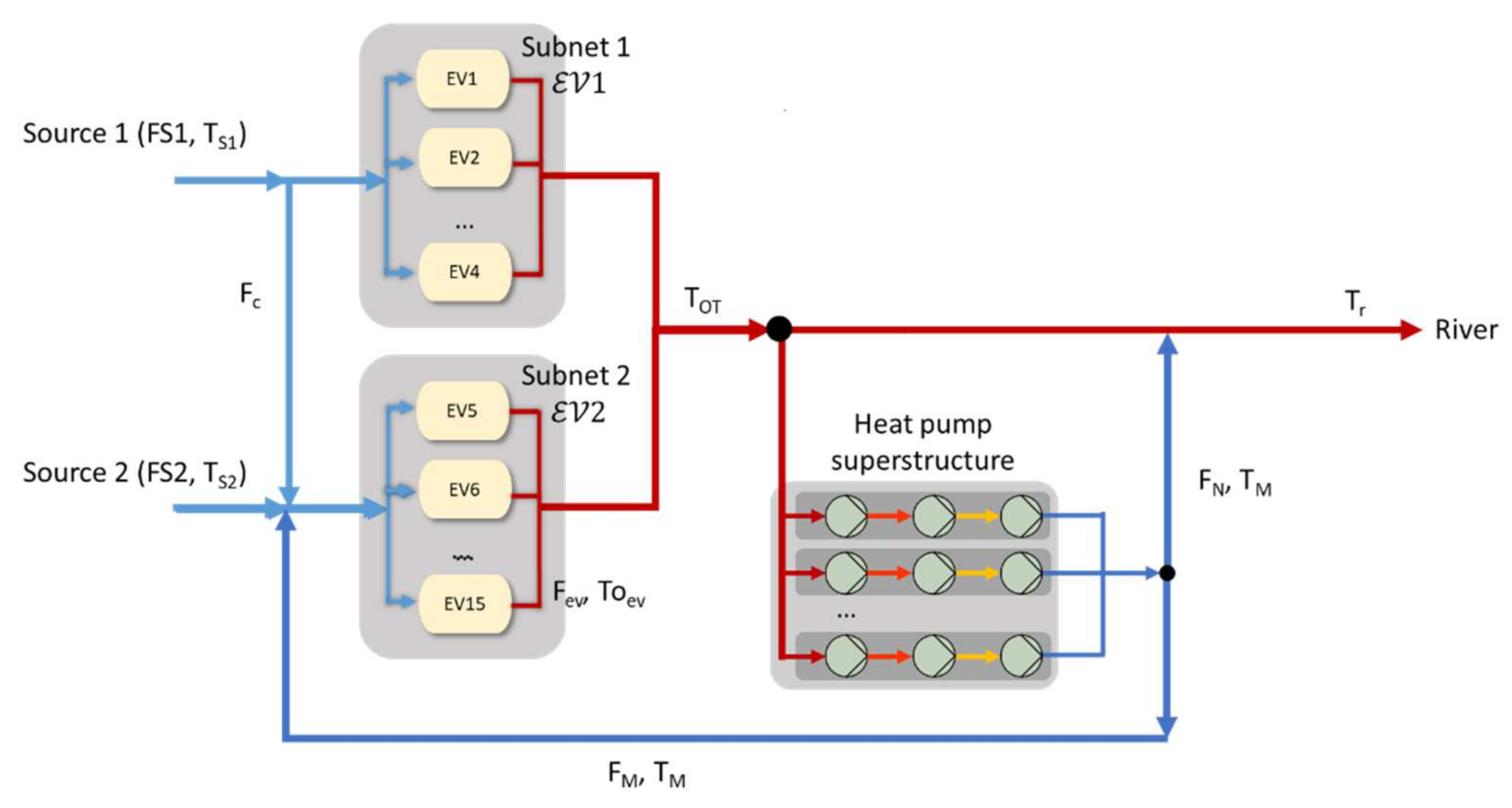
The cooling system associated to each evaporation plant is based on surface condensers (see Figure 1a) and, according to the source of the cooling water (resource) fed to the condenser, the evaporation plants can be grouped in two sub-networks. The first one, formed by four evaporation plants, can only get cooling water from Source 1, meanwhile the subnet two, formed by the remaining eleven plants, can get cooling water from both sources (see Figure 1b). However, note importantly that the cooling water to take from each source is limited, so a problem of shared resources arises. Furthermore, as the outlet cooling water goes back to a river, its temperature must be below a limit imposed by environmental regulation.
Note that both networks (spinbath processing and cooling-water distribution) are coupled, so their operation is coupled too. In previous works, we have addressed the optimal evaporation load allocation considering the demand of each product for a given cooling power [16], and the optimal cooling water distribution for a given evaporation load according to the available water at the sources [17]. Furthermore, we have also studied ways to efficiently formulate and solve the optimization of the whole coupled system in real time, i.e., the spinbath allocation and water distribution [18].
In this work, we go beyond joint operation of the interconnected networks by studying process design decisions as well. In this regard, the previous mathematical formulation to solve the real-time optimization problem is twofold extended: (a) to include the possibility of attaching heat pumps to the cooling system in order to improve the overall resource efficiency; and (b) incorporating uncertainty in future operation conditions.
3. Network Model
This section presents the design specifications, operational constraints, and the mathematical model to represent the entire network.
3.1. Problem Statement
In brief, a heat pump (HP) is a thermal machine that extracts heat from a fluid and transfers it to another. In our case, we want to cool down the outlet cooling water from surface condensers (SC), so HPs must be placed after SCs in a way that the SCs outlet flows are mixed and feed to HPs. Thereupon, the task here is to investigate which is the best way to incorporate HPs in the cooling network such that the cooling capacity is improved (hence, operability margins in the evaporation section too) while fulfilling environmental regulations, but without incurring in an excessive time lag between investment and payback.
Specifically, there are three main questions to answer:
- How many heat pumps are needed to be installed?
- Which is the best installation layout, i.e., connections among them?
- How the HPs should be incorporated into the actual network layout?
In this regard, connection among heat pumps can be::
- In series: the input flow of an HP is the output of the previous one.
- In parallel: all HPs receive an inlet from the same stream.
- Hybrid: a combination of the above as a matrix of HPs, where some HPs are arranged in series forming blocks that are connected in parallel.
Note that the first two options are particular cases of the hybrid one, so the mathematical model is developed to account for this general layout in the design optimization.
With respect to the outlet flow from the HP system, there are two options:
- To be mixed with the remaining outlet flow from the SCs (amount that could not be directed to the HPs), in order to decrease the temperature of the water flow that goes to the river.
- To be mixed with the inlet flow of the surface condensers (i.e., like it is an additional water source). However, note that this option is only possible for the evaporation plants in Subnet 2, because circulation of water from Source 2 to Subnet 1 is forbidden (see Figure 1).
Furthermore, as the heat pumps may be connected in serial blocks, both options must be regarded for each block. Figure 2 shows a schematic of the modified network layout according to these proposed options.
In summary, there are quite a few decisions to take on the HPs integration design side, added to those related to the operation of the existing evaporation network (Section 2). Note that the HP add-on is to be designed in such a way that optimizes operation of the complete system in the more usual situations along the year. In this regard, although there are detailed models and performance studies on HPs available in the research literature [19], only nominal features are often considered at this industrial level. Then, HPs are placed in such a way that they operate at (or close to) design conditions. Therefore, with the aim of not adding unnecessary complexity to our mathematical formulation, in this paper we neglect the dynamics, and we characterize an HP simply by:
- Its capacity, i.e., the heat flow that is able to transfer from one fluid to the other (Q),
- Its energy efficiency ratio (EER), that is the ratio between the capacity and the electrical power consumption required to achieve it,
- The nominal flow FB, for which the HP achieves its capacity in steady state.
Hence, in our case study we can roughly model an HP by its energy balance where Cp and are the specific heat and density of the cooling water through the HP respectively, and ΔT is the temperature difference between the inlet and outlet.
It is worth mentioning that the heat pumps remove heat from the desired streams and such heat could be used. Nevertheless, in this work the possible uses for such heat are left out of the optimization, even though they would bring extra savings.
3.2. Mathematical Formulation
The formulation of the mathematical model which represents the superstructure of the network operation is based on the work of [18]. Here we adapted it in order to incorporate the corresponding modifications to include decisions on HPs integration.
3.2.1. Sets
First, we defined the different sets which we are working with.
- : set of all the evaporation plants. This set is divided in two subsets according to the existing SCs subnet arrangement, i.e., those that have access to cooling-water Source 2 or not.
- : set of all the different products: set of the blocks of heat pumps, to be connected in parallel.
- : set of heat pumps connected in series within each block. All blocks have the same maximum number of heat pumps, denoted by .
3.2.2. Decision Variables
The variables that relate the above introduced sets are now defined:
- ℝ+: evaporation load of product p that plant ev must achieve.
- {0,1}: indicates if the product p is treated in plant ev
- ℝ+: cooling-water flow that goes to the plant ev
- {0,1}: indicates if a heat pump hp in block b is in operation () or not ()
- ℝ+: recirculated flow to the surface condensers after the heat pumps.
- ℝ+: flow that goes to the river after the heat pumps.
3.2.3. Model Constraints
The constraints of the model that represent the operation of the evaporation network in steady state are based on first principles and some logic statements, detailed below. In this formulation, italic symbols represent variables and sets whilst plain ones are known values (i.e., inputs or parameters) for the optimization.
- 1.
- An evaporation plant only can process as much one product at a time:
- 2.
- There are some impossible connections between plant and products (see Table 1):
- 3.
- The connection in series of the heat pumps imply that in order to use the next heat pump of the chain, the previous one must be connected:
- 4.
- In the same way, to avoid different solutions with the same number of heat pumps we force to connect a heat pump of a block only if the heat pump of the previous block in the same position in the chain is connected:
- 5.
- The outlet flow of heat pump matrix can be recirculated to the SCs inlet or delivered to the river stream:
In (6), FB is the flow that goes through each block of HPs, whose value is the same for all the heat pumps (all the HP have the same features) and it is set by the nominal specifications of the HP. As it is a fixed parameter, to assure that there is flow passing through the block, we multiply it by the sum of , as due to (5) if any heat pump of a block is connected the first heat pump of the chain must be connected.
- 6.
- The evaporation demand for each product must be fulfilled:where parameter SPp denotes the evaporation setpoint for product p required by the factory in order to fulfill the demand.
- 7.
- The evaporation load in each plant is bounded due to actual equipment features:where and state the minimum and maximum evaporation load for a plant to operate correctly. With we assure that take zero value for the products not linked to plant ev.
- 8.
- The cooling water flow through the surface condenser is also bounded:where and states de minimum and maximum cooling-water flow that could pass through the surface condenser attached to the evaporation plant ev. Similar to the previous constraint, we force that the cooling water flow is zero if there is not any product linked to the evaporation plant, in this case through added for all products.
- 9.
- Mass balance of cooling water in each subnet. The total flow that feeds the surface condensers of plants in Subnet 1 must be, as maximum, the available flow at Source 1 (FS1) minus the flow that goes to Subnet 2 (Fc). In subnet 2, there are three inputs of cooling water: Source 2 (FS2), remaining water from Source 1 (), and the flow recirculated from HPs ().
- 10.
- Energy balance for each heat pump:where Q, FB, Cp and are as in (1), and is the temperature difference between the flow inlet and outlet in each HP. Note that the temperature difference is set by (12), so we can rewrite it as in (13) where the outlet water temperature at each HP () can be computed from the inlet one. That is directly the outlet of the previous HP connected in series ()
By this method, if a heat pump is not connected (), the outlet temperature is the same as the inlet one. Note that for the first HP in each block, is the temperature resulting from the mixture of flows leaving the SCs ().
The outlet water temperature of each SC () is computed with the data-based model (14) developed in [17] according to the inlet water temperature (), the flow () and the state of fouling () of the SCs, which can be estimated online.
where is a polynomial function to compute the increment of temperature in the SCs according the flow through them. The functions were obtained through regression with experimental data (details omitted for brevity). Note that depends on the known water source temperatures ( and ), but also on the temperature of the water potentially recirculated from the HP section (mixture of the outlets from each HPs block that is chosen to recirculate water via ):
where, according to its definition in Section 3.2.1, sub-index refers to the last HP in block b.
- 11.
- The stream temperature that goes to the river, in Figure 2, should be below that the maximum temperature allowed by environmental regulation (MTO):
The stream is the mixture between the SCs outlet that does not feed the HPs, and the outlet of the HP blocks that is not recirculated to the SCs inlet via , whose temperature is the same as the recirculated one, :
4. Network Design
Once the mathematical model which represents the system has been described, we can formulate an optimization problem in order to know the optimal number of HPs to be installed for a set of the most usual operation scenarios (stochastic optimization), according to an economic criterion and considering the payback time.
4.1. Optimization Problem
The operation cost of the network could be computed as the sum of three different terms: the cost due to the steam consumption in the evaporation plants, the one associated to the cooling-water consumption, and the cost of the electricity consumed by the heat pumps.
In [16], Kalliski and co-authors built a data-based model to estimate the steam consumption of an evaporation plant according to some key factors: the evaporation demand , the plant state of fouling , and the water temperature leaving the cooling system . Nevertheless, in the system described in that paper, the evaporation plants owe independent cooling towers as cooling systems, whilst here the cooling systems are SCs connected through the water-distribution network. Note that, in a SC, a single temperature measurement at the SC outlet does not fully determine the actual cooling power: both the inlet-water flow and temperature vary over time, whilst a cooling tower runs with the nominal flow cooled down to a controlled temperature setpoint (what varies over time is the air flow through the tower).
Consequently, we were forced to adapt the models in [16] using the actual cooling power (computed as (20) shows) instead of the outlet-water temperature as input.
The plants fouling states () are estimated online following an analogous procedure to the one for in (14), see [16,20] for details. Note that refers to the fouling state of the evaporation plants whilst refers to the fouling state of the surface condensers; nevertheless, both are periodically estimated from real-time plant data and treated as known input values in the optimization. Hence, the absolute steam consumption (ASC) at each evaporation plant can be predicted by (21), where θ := {α, β, γ} are the model parameters.
The steam-consumption contribution to the total cost () is computed then as the overall ASC times the price of generating a unit mass of live steam in boilers () as (22) shows. In the same way, the cooling-water cost () is the net amount of water consumed from the sources times the cost of pumping and pipes operation (). The electric power consumed by the connected HPs is known from their capacity and Energy Efficiency Ratio (EER).
Thus, the objective function to minimize is the operation cost, which is given by the sum of the three terms:
Furthermore, we must consider the price of each equipment and when they will be amortized. Hence, we added a constraint to consider the payback time (RP), which has to be the one required from the company as maximum. The payback is computed as the price of the heat pumps (according to [21], a reasonable price for this kind of heat pump is EUR 40,000, each one (PHP)) divided by the savings over a year, where such savings can be computed as the difference between the operation cost of the current network () and the new cost with heat pumps predicted by the model (OF).
Note that the potential savings obtained by using heat pumps could be higher than the values computed here, as the heat removed from the outlet stream might be used in other section of the plant.
4.2. Model Parameters
In many of the above model constraints there are parameters whose value is fixed and known, and measurable inputs which depend on the operating conditions.
For the specific heat and density of the cooling water we assume constant values in the plant operation range, kJ/kg and kg/L, respectively.
The prices of steam, cooling water and electricity are calculated internally in the company, so their values are omitted here due to confidentiality agreements.
The HPs selected capacity (Q = 500 kW) and the energy efficiency ratio (EER = 4) were taken from the spec sheets provided by the manufacturers of these equipment [21,22,23]. Note that the number of heat pumps to use and their layout are decision variables in the model, but the maximum number of HP to install depends on the elements stated for sets and . For this case study, we have estimated that 15 blocks () with 3 HPs each (, 45 HPs in total), provide enough design flexibility to find optimal solutions. If the results of the optimization would indicate that either all heat pumps in a row or fifteen heat pumps in parallel are required, such sets would be expanded.
Finally, the water availabilities at the two sources and their temperatures, the state of fouling of each evaporation plant, and the demand of each product, can change over time. Thus, different scenarios have been posed accordingly, in order to take into account different expected operation conditions. Note that the cost of operating the network without heat pumps also depends on the value of these parameters and conditions so, to be fair, it will be computed also via optimization with the proposed model, but forcing no inclusion of HPs.
4.3. Two-Stage Stochastic Formulation
The aim of stochastic programming is to find optimally robust decisions in problems that involve uncertainty. In this case, the main objective is to know how many heat pumps to buy, considering that there are some input variables in the model whose future evolution is uncertain. Hence, these model inputs are treated as stochastic variables and, in a finite-dimensional formulation, different scenarios arise according to the different values considered in the variables, representing some probable future uncertainty realizations.
Table 2 summarizes the scenario set that has been considered for this case study according to the model inputs that are subject to variability. The scenarios have been built from the most common conditions observed in historical data recorded over a year of operation (mean values), plus adding the worst possible cases. φ indicates the percentage realization probability of each scenario respect to the rest.
Note that there are two scenarios (n° 7 and 8) where it is not possible to fulfil all the constraints without heat pumps for the given operation conditions (infeasible problems). Thus, the payback computation (26) cannot be performed for these scenarios ( in cannot be computed). Nevertheless, note that they will be included in the design optimization anyway (in the objective function and rest of model constraints). Moreover, as the sum of their realization probability is lower than 3%, excluding them from the payback constraint will not vary the economic estimations significantly.
Following the two-stage stochastic approach, we consider that only the number of heat pumps to purchase () is the first-stage variable (here and now decision) and the rest of variables in the model are of second stage, as they can be adapted to each uncertainty realization (recourse variables). Thus, all these variables and the involved constraints are extended with a new sub-index that refers to the scenario numbers listed in Table 2 (e.g., the evaporation load now will depend on the evaporation plant ev, the product p, and the scenario i: ).
4.3.1. Monolithic Formulation
It may happen that the optimal number of heat pumps to switch on in a particular scenario could be lower than the purchased heat pumps, i.e., using all the installed heat pumps could not be economically optimal if water availability and temperature are favorable for instance. Hence, N can be defined as the maximum number of heat pumps used in all scenarios, as (27) shows.
To define the payback constraint, we can follow different approaches depending on the robustness level we want to consider. It is clear that the payback time horizon has to be computed with the number of purchased heat pumps, but this constraint could be applied for each scenario (hence it would consider the worst case) or just once, computing the weighted average for the different cases according to the probability φ assigned to each one. In the proposed formulation we followed this second approach, so (26) is rewritten as (28):
Finally, the objective function to minimize is the weighted sum of the operation cost for each scenario according to its probability. Therefore, the resulting two-stage stochastic optimization problem is summarized by:
The results of the optimization will give the optimal number of heat pumps to purchase as well as, for each scenario: the HPs to be used and their connection layout, the cooling-water distribution, and the product allocation to plants. Everything assuring the average payback time RP in (28) is fulfilled.
Nevertheless, the presence of discrete and continuous variables as well as the nonlinear dependency among them in many constraints, make (29) be a non-convex mixed integer nonlinear programming (MINLP) problem, with a relatively high number of decision variables. In order to overcome the typical issues of slow solution convergence and high computational demands in a centralized formulation, we propose a suitable problem decomposition.
4.3.2. Decomposed Formulation
The reader may have noted that the only shared variable among all scenarios in the optimization problem (29) is the number of heat pumps to buy (N), arising in the payback complicating constraint. Thus, removing (28), the optimization of each scenario minimizing subject to (2)–(18) can be solved independently, hence computed in parallel. Therefore, the key is to develop an upper-layer master problem to ensure the payback constraint.
The payback time can be computed once the results of each scenario are obtained, and then be compared with the desired RP value. However, this simple calculus does not ensure that the constraint is fulfilled. To solve this, an iterative procedure could be applied. First, each scenario is solved independently and, with the locally obtained results, (27) and (28) can be computed. If (28) is fulfilled, that is it, an optimal solution is reached. (of course, the provided guarantees are just for local optimality if gradient-based MINLP solvers are used, as the problem is non-convex). If not, the available number of heat pumps to use needs to be lower than the suggested in the current iteration k. To impose this, we incorporate the new constraint set (30) onto the model that forces the maximum number of heat pumps to use is lower than a predefined parameter , whose value has been obtained by (27) in the previous iteration () and updated to .
In the next iteration, we will have the results of each scenario according to this constraint, so the master problem can check again if (28) is fulfilled. This iterative procedure is formalized in Algorithm 1 below.
| Algorithm 1. Decomposed iterative optimization |
| 1: Set and minimize subject to (2)–(18) for all scenarios 2: Compute through N defined in (27) 3: While (28) is not fulfilled do: 4: 5: Minimize (25) subject to (2)–(18) and (30) for all scenarios 6: Compute the overall weighted operation cost of (30) from the scenario costs obtained in Step 5 7: Go back to Step 2 |
Note that decomposition approach provides (local) optimality guarantees because: parameter only can take non-negative integer values; and RP is monotonic with respect to , i.e., the payback time increases with the number of purchased heat pumps. This is because (28) is affine in and the savings increment provided per year attenuate with the number of purchased HPs, see results in next section. In fact, thanks to these features, Algorithm 1 converges to a solution in, at most, iterations.
Note that this procedure is equivalent to the stochastic centralized formulation (30) but the computational demand and time to obtain a solution is significantly reduced, as the scenario optimizations in each iteration are solved independently, in a simultaneous fashion if parallelized. Thus, the computation time in each iteration is the one of the most demanding scenario.
4.4. Results
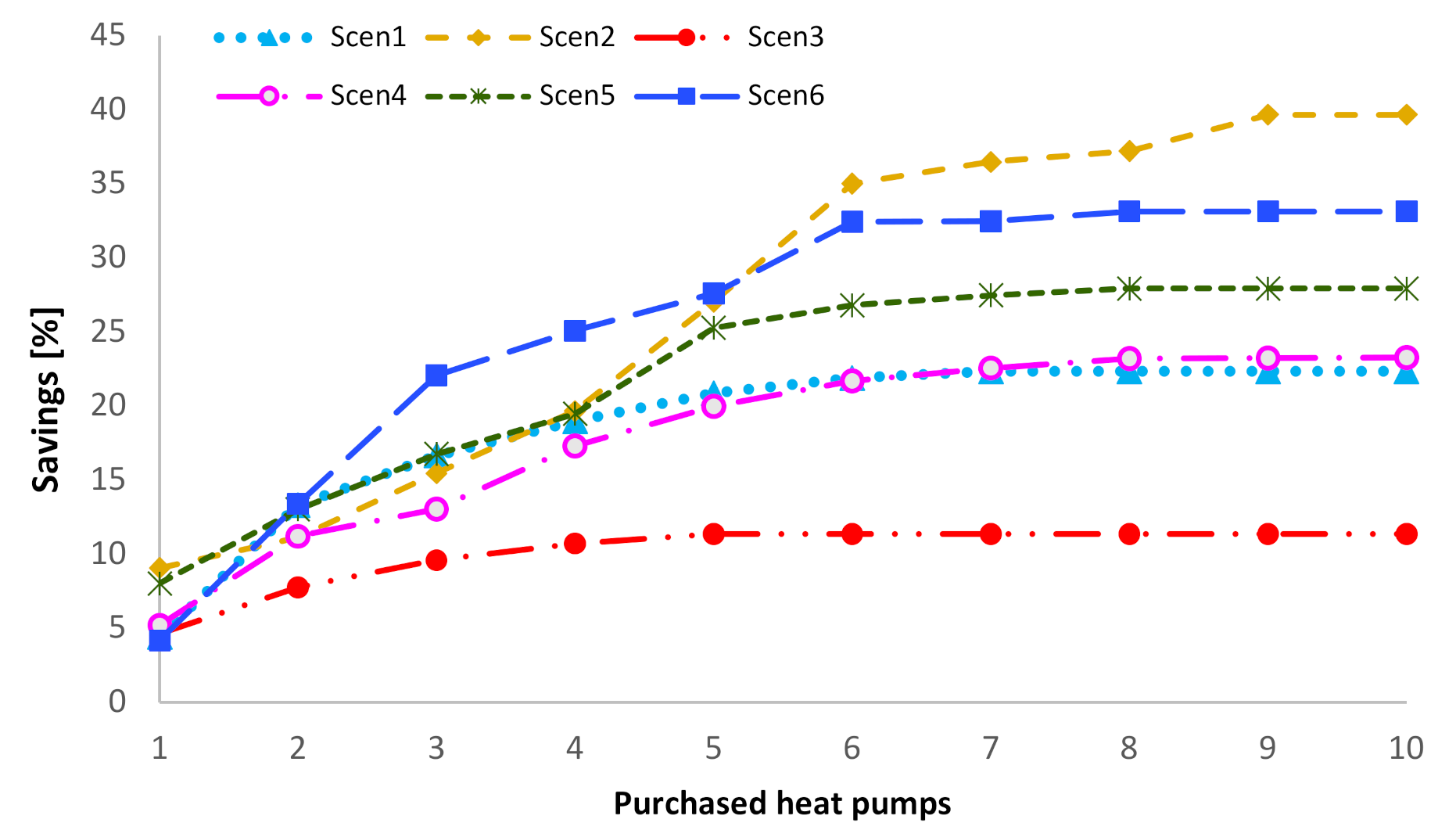
Following the methodology described in the previous section, we have obtained the results showed in Figure 3 and Figure 4, where the percentage of savings is the difference between the operation cost of the current network () and the new cost with heat pumps predicted by the model (), normalized by the current cost ().
The behavior of the system is that, as more cooling water goes through the SCs, the more efficient the evaporation plants are and, consequently, the less steam consumption is needed by them to achieve the evaporation demand. Consequently, the more heat pumps, the more cooling water may be recirculated and available to use it in the SCs. Nevertheless, at some point, the savings for the reduction of steam consumption are not high enough to compensate the electricity costs to switch on many heat pumps. Hence, each scenario has a different amount of heat pumps on to reach optimal operation, i.e., the lowest operation cost.
In this regard, the numbers in Figure 3 show how the percentage of savings obtained in each scenario increases with the number of purchased HPs, but only until the optimal number of HPs switched on is reached. Thus, when the purchased HPs exceeds the number of those that are optimal for a scenario, the savings remain constant.
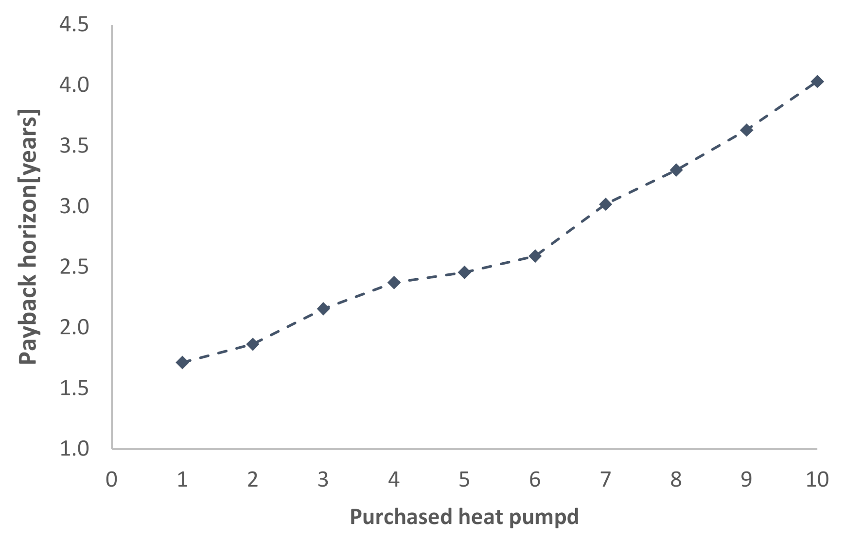
If we focus in the payback time, showed in Figure 4, it increases with the number of purchased HPs, as expected due to the monotonic behavior of (28) with respect to . Although buying more HPs increases the savings, they progressively loose influence to compensate the increased initial investment, so that the payback time also increases. In addition, this increment is not linear and vanishes with as the number of HPs increases. Hence, when a scenario reaches its highest possible savings, increasing the purchased HPs will only increment the payback time.
Note that Figure 3 and Figure 4 depict values in a range . This is because the first iteration applying Algorithm 1 already computed , i.e., the highest number of used heat pumps was 10, obtained for Scenario 4. Therefore, purchasing more HPs does not make sense because it does not translate in more steam savings, as the trends in Figure 3 clearly show. From that upper value, we followed the proposed procedure, decreasing N in each iteration until just to show a complete view of the system behavior. For the actual case, where RP must be as maximum 3 years, the number of heat pumps to buy is six, stopping the algorithm after five iterations. This choice predicts obtaining 22.7% average steam savings. Note that some scenarios would obtain more savings with more heat pumps, but their realization probability is not enough to compensate the required investment to be amortized in three and a half years. Nonetheless, the door to buy and additional HP in the future is open if conditions vary.
It is important to note that scenarios 7 and 8, which are not included in the payback computation, are indeed feasible with HP integration. In this way, investing in HP integration can assure not only mere resource savings but also that the site would keep production capacity in extreme conditions, what is not possible currently.
Additionally, note that although the optimal number of HPs to purchase is six, the optimal number of them to switch on will vary with time, according to the operation conditions.
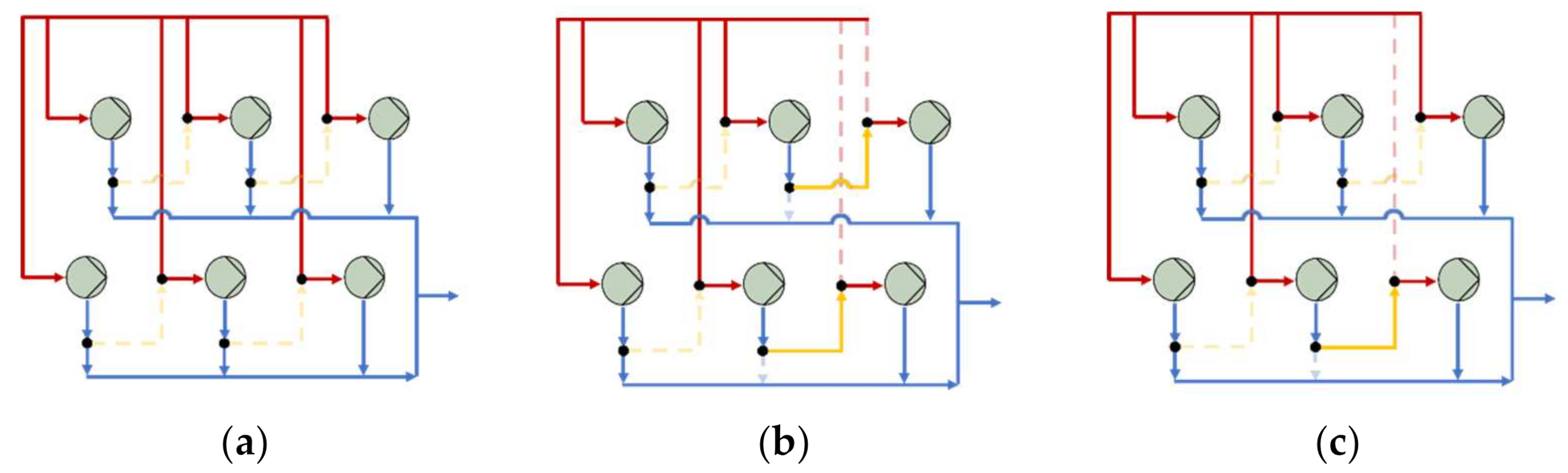
With respect to the installation layout, for scenarios 1 to 6 the optimizer chooses to connect all suggested heat pumps in parallel (Figure 5a). Nevertheless, for scenarios 7 and 8, the layout would be:
Therefore, the proposed installation layout is a matrix of six heat pumps, initially connected in parallel, but with two of them having the possibility to drive its outlet into the inlets of other two, in order to connect these HPs in series. This piping configuration is easily implementable with on/off valves in the entries and outlets of the involved heat pumps (represented with a black circle in Figure 5).
Finally, the only question that remains open is how the HPs should be incorporated into the actual network layout, regarding what to do with the outlet flow from the HPs section. For most scenarios, the suggestion for such a flow is complete recirculation to the inlet of Subnet 2. Nonetheless, when the inlet temperature from the sources is quite high, or in the hypothetical cases where the maximum temperature allowed by the environmental regulation (MTO) decreases, the computed results suggest recirculating only part of the flow as the most beneficial course of action. The remaining part will join the water going to the river. Therefore, the optimal installation design is to incorporate a flow control valve at the outlet of the HPs section, able to modify the flow that goes each way, i.e., the values of FM and FN in Figure 2.
5. Network Optimal Operation
Once the incorporation of the new equipment into the network is designed, the only remaining issue is to operate the network in the best efficient way. In addition to know the evaporation load that each evaporation plant must process regarding the demand of the different products, and the cooling water distribution according to the to the availability of the sources, now it is also needed to know how many HPs connect, as it depends on the actual conditions arising in real time. This kind of problem is too complex for a human operator/manager due to the large number of alternatives arising from the combinatorial problem. In the best case, the human network driver would find a set of control set points based on its experience that is suboptimal, looking just for a feasible one in the worst case. Therefore, a decision support system (DSS) with embedded model-based mathematical optimization is desirable to help in this daily task.
5.1. Real-Time Optimization
Here, we will widen the solution provided in [18] in order to take into account the incorporation of heat pumps. The increment of available cooling water due to the heat pumps not only would change the cooling-water distribution but also might change the load allocation. Furthermore, we need to incorporate the decision of how many heat pumps to connect in the RTO formulation.
Hence, we reuse the mathematical formulation of the previous section to develop an RTO tool that determines the optimal operation set points according to the real-time conditions. The optimization problem to solve is the same as the one in the decomposed approach for a particular scenario realization, i.e., to minimize the total cost of operating the network subject to (2)–(18) and (30), taking into account that in (30) is now fixed to six. Furthermore, to speed up the resolution by decreasing the number of useless decision variables by setting that the set only includes 6 elements () and set will include just three elements (), according to the layout configuration of Figure 5.
The parameters and input values which depend on the operation conditions (the availability of the cooling water sources and their inlet temperatures, the fouling states of plants and SCs, and the demand of the different products) will be supplied to the RTO by the site information technology (IT) system. As the RTO is coded in Pyomo—Python, one way to do that would be through PIconnect [24], which grants access to the OSISoft Plant Information (PI) system to update the needed data. Currently, as the purchase of HPs is not yet materialized, the RTO has been tested off-line, accessing to the historical plant data in the PI system. Nevertheless, it could actually access the PI system in real time to automatically get current values of the plant variables in a kind of what-if analysis fashion.
Using six heat pumps, the number of decision variables in the RTO is 186, from which 93 are binary. As for RTO we require obtaining solutions in short time periods, we have used the NLP-based branch-and-bound algorithm Bonmin [25], at the price of possibly reaching a local optimum from time to time.
With this setup, the average time to get a solution with zero relative gap (in nonconvex MIP this value is just informing that the branch-and-bound process ended, but it does not mean that the global optimum is found) is ~20 s in an i7 Intel CPU workstation. This computational time is considered suitable, as the frequency to account for sensibly observable changes in the evaporation demand or sources availability is more than twenty minutes.
5.2. Human–Machine Interface Design
As the final aim of the RTO is to support operators and plant managers on the daily management of the network, we need to provide them with a friendly interface where the results of the optimization translate also into clear directives to perform by the human. Thus, the person in charge can take a look at the presented suggestions and combined with his expert knowledge, decide how to proceed.
According to the plant personnel preferences, we designed the interface in MS Excel. It displays the important information and suggested actions, previously computed by the RTO in the backend. The connection between Python and MS Excel is done via OpenPyXL [26]. It is noteworthy that this is a bi-level interface, where plant engineers have further access to modify some optimization parameters and model coefficients in case that something in the network layout changes (for example incorporation another heat pump).
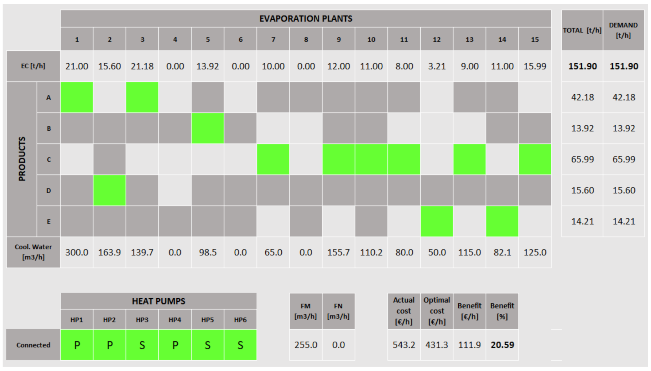
The interface developed for the operator extends the one they already have to manage the plants evaporation load: it shows the solution obtained with the RTO on a dashboard. Figure 6 shows an example with the results obtained for some conditions read from historical data, as the tool has not been implemented yet.
Note in the picture that there is a two-column panel at the right side. The first column indicates the total evaporation load processed by all the plants, and the second one is the evaporation demand for each product. These two need to match for the allocation to be right. At the bottom we have included three more display panels. The first one on the left indicates if each heat pump should be switched on (also in green) and how it should be connected, displaying a P if the connection is in parallel or an S if it is in series. If the heat pump should be off, the cell will be in dark gray. The next panel shows the flow that should go to each side after the heat pumps (to be recirculated o to be mixed with the outflow that goes to the river).
Finally, the right-side panel shows the total cost of operating the network in the current conditions versus the cost predicted with the proposed distribution. Moreover, the savings that will be presumably achieved by applying the optimized distribution are explicitly displayed in order to encourage the operator to follow the recommendations proposed by the tool.
6. Remarks and Outlook
In this paper we revisited two important problems in process systems engineering from an integrated perspective: the optimal design for the incorporation of new equipment into an existing facility, and the optimal operation of the modified system.
Our approach is in line with the ideas brought up by the digitalization and the so-called Industry 4.0 paradigm, providing useful information from process knowledge and collected data, and making it accessible in a comprehensible way for the plant personnel.
Taking an industrial network of evaporation plants in a viscose-fiber production facility as the example to illustrate these ideas, we first developed a rigorous mathematical model of the network including all the possible layouts of the new equipment to be incorporated, as well as of its potential connections. Based on this model, we have formulated an optimization problem which indicates the optimal layout of the equipment in such a way that the operation cost of the whole network would be minimum. However, as the results depend on the operation conditions, whose future realizations are somehow uncertain, we built a two-stage stochastic formulation with different scenarios that intend to cover reasonably the plausible operation conditions. The first approach was to formulate the optimization problem in a monolithic way, but due to the characteristics of the resulting optimization problem (MINLP problem), we proposed an equivalent decomposed approach. Such an approach is possible because the individual formulations for each scenario are only linked by a single constraint (payback time horizon) involving a shared variable (number of HPs to purchase). Moreover, as the shared variable is an integer positive number and the payback-time constraint is monotonic with such a variable, the solution is proven to be obtained in few iterations with the proposed algorithm for decomposition of the monolithic problem.
Analyzing the solutions, we got the best configuration considering the payback time that the company considers acceptable. In general, the benefits increase with the number of used heat pumps, up to an extent, as more recirculated water involves lower steam consumption. However, at some point the reduction cost of steam does not compensate the electrical cost of installing more heat pumps. It is worth mentioning that the optimal number of heat pumps to use and its layout depend on each scenario.
Consequently, once the optimal design is found considering the operating conditions, the daily operation is to be addressed. For such a task, an RTO was built based on the same model of the network, already developed. From the current plant situation (real-time collected data), this tool suggests the optimal connection of heat pumps, the evaporation-load allocation and the cooling-water distribution according to an economic criterion. Consequently, the proposed system architecture is able to quickly react to disturbances or load changes. Nevertheless, the human operator needs to be in the loop, so a tailored HMI that displays the key information computed by the RTO needs to be provided in order to ease the visualization of the results and to help him/her in this complex decision-making process. However, in our case study such a tool has not been tested online in the site, as the company is still evaluating the acquisition of the heat pumps. Therefore, that will be the next step as soon as the site is ready.
Author Contributions
Conceptualization, J.L.P. and C.d.P.; methodology, M.P.M. and J.L.P.; software, M.P.M.; validation, M.P.M. and J.L.P.; formal analysis, M.P.M. and J.L.P.; investigation, M.P.M. and C.d.P.; resources, C.d.P.; data curation, M.P.M.; writing—original draft preparation, M.P.M., J.L.P. and C.d.P.; writing—review and editing, M.P.M., J.L.P. and C.d.P.; visualization, M.P.M.; supervision, J.L.P. and C.d.P.; project administration, C.d.P.; funding acquisition, C.d.P. All authors have read and agreed to the published version of the manuscript.
Funding
These results received funding from the Spanish MICIU with FEDER funds under project InCO4In (PGC2018–099312-B-C31) and by the regional government of Castilla y León and the EU-FEDER (UIC 223 and CLU 2017-09). The first author thanks the European Social Fund and the “Consejería de Educación de la Junta de Castilla y León”.
Acknowledgments
The authors gratefully acknowledge Alexander Arnitz from Lenzing AG for the fruitful collaboration and sharing its knowledge on heat pumps.
Conflicts of Interest
The authors declare no conflict of interest. The funders had no role in the design of the study; in the collection, analysis, or interpretation of data; in the writing of the manuscript, or in the decision to publish the results.
References
- de Prada, C.; Mazaeda, R.; Podar, S. Optimal operation of a combined continuous–batch process. In Computer Aided Chemical Engineering; Elsevier: Amsterdam, The Netherlands, 2018; Volume 44, pp. 673–678. [Google Scholar]
- Liong, S.-Y.; Atiquzzaman, M. Optimal design of water distribution network using shuffled complex evolution. J. Inst. Eng. 2004, 44, 93–107. [Google Scholar]
- Grossmann, I.E.; Floudas, C.A. Active constraint strategy for flexibility analysis in chemical processes. Comput. Chem. Eng. 1987, 11. [Google Scholar] [CrossRef] [Green Version]
- Birge, J.R.; Louveaux, F. Introduction to Stochastic Programming; Springer: New York, NY, USA, 2011. [Google Scholar] [CrossRef]
- Steimel, J.; Engell, S. Conceptual design and optimization of chemical processes under uncertainty by two-stage programming. Comput. Chem. Eng. 2015, 81. [Google Scholar] [CrossRef]
- Krämer, S.; Engell, S. Resource Efficiency of Processing Plants: Monitoring and Improvement; John Wiley & Sons: Hoboken, NJ, USA, 2017. [Google Scholar]
- Rashidi, M.; Ghodrat, M.; Samali, B.; Mohammadi, M. Decision Support Systems. In Management of Information Systems; Pomffyova, M., Ed.; IntechOpen: Rijeka, Croatia, 2018. [Google Scholar]
- Hernandez, R.; Dreimann, J.; Vorholt, A.; Behr, A.; Engell, S. Iterative real-time optimization scheme for optimal operation of chemical processes under uncertainty: Proof of concept in a miniplant. Ind. Eng. Chem. Res. 2018, 57, 8750–8770. [Google Scholar] [CrossRef]
- Galan, A.; de Prada, C.; Gutierrez, G.; Sarabia, D.; Grossmann, I.E.; Gonzalez, R. Implementation of RTO in a large hydrogen network considering uncertainty. Optim. Eng. 2019, 20, 1161–1190. [Google Scholar] [CrossRef] [Green Version]
- Merino, A.; Acebes, L.F.; Alves, R.; de Prada, C. Real Time Optimization for steam management in an evaporation section. Control Eng. Pract. 2018, 79, 91–104. [Google Scholar] [CrossRef]
- Ferreira, T.d.; Wuillemin, Z.; Marchetti, A.G.; Salzmann, C.; van Herle, J.; Bonvin, D. Real-time optimization of an experimental solid-oxide fuel-cell system. J. Power Sources 2019, 429, 168–179. [Google Scholar] [CrossRef]
- Marcos, M.P.; Pitarch, J.L.; de Prada, C. Decision support system for a heat-recovery section with equipment degradation. Decis. Support Syst. 2020, 137, 113380. [Google Scholar] [CrossRef]
- de Prada, C.; Sarabia, D.; Gutierrez, G.; Gomez, E.; Marmol, S.; Sola, M.; Pascual, C.; Gonzalez, R. Integration of RTO and MPC in the Hydrogen Network of a Petrol Refinery. Processes 2017, 5, 3. [Google Scholar] [CrossRef] [Green Version]
- Palacín, C.G.; Pitarch, J.L.; Jasch, C.; Méndez, C.A.; de Prada, C. Robust integrated production-maintenance scheduling for an evaporation network. Comput. Chem. Eng. 2018, 110, 140–151. [Google Scholar] [CrossRef]
- Pitarch, J.L.; Palacín, C.G.; Merino, A.; de Prada, C. Optimal operation of an evaporation process. In Modeling, Simulation and Optimization of Complex Processes HPSC 2015; Springer: Berlin/Heidelberg, Germany, 2017; pp. 189–203. [Google Scholar]
- Kalliski, M.; Pitarch, J.L.; Jasch, C.; de Prada, C. Support to decision-making in a network of industrial evaporators. Rev. Iberoam. Automática E Inf. Ind. 2019, 16, 26–35. [Google Scholar] [CrossRef] [Green Version]
- Marcos, M.P.; Pitarch, J.L.; de Prada, C.; Jasch, C. Modelling and real-time optimisation of an industrial cooling-water network. In Proceedings of the 2018 22nd International Conference on System Theory, Control and Computing (ICSTCC), Sinaia, Romania, 10–12 October 2018; pp. 591–596. [Google Scholar]
- Marcos, M.P.; Pitarch, J.L.; Jasch, C.; de Prada, C. Optimal distributed load allocation and resource utilisation in evaporation plants. In Computer Aided Chemical Engineering; Elsevier: Amsterdam, The Netherlands, 2019; Volume 46, pp. 979–984. [Google Scholar]
- Chua, K.J.; Chou, S.K.; Yang, W.M. Advances in heat pump systems: A review. Appl. Energy 2010, 87, 3611–3624. [Google Scholar] [CrossRef]
- Lenzing. D2.5 Final Report on Equipment Degradation Modelling. 2019. Tech report, Outcomes of the CoPro project. Available online: https://ec.europa.eu/research/participants/documents/downloadPublic?documentIds=080166e5c438f3a5&appId=PPGMS (accessed on 18 June 2021).
- De Kleijn Energy Consultants & Engineers, “Industrial Heat Pumps”. 2014. Available online: http://tools.industrialheatpumps.nl/warmtepompwijzer/EN_index.html (accessed on 3 November 2020).
- Danfoos Engineering Tomorrow, “Coolselector 2”. Available online: https://www.danfoss.com/es-es/service-and-support/downloads/dcs/coolselector-2/ (accessed on 3 November 2020).
- Ochsner Energie Technik. Available online: https://ochsner-energietechnik.com/hoechsttemperatur-waermepumpen/ (accessed on 3 November 2020).
- den Berg, H. PIconnect 0.8.0. 2020. Available online: https://pypi.org/project/PIconnect/ (accessed on 20 February 2021).
- Bonami, P.; Biegler, L.T.; Conn, A.R.; Cornuéjols, G.; Grossmann, I.E.; Laird, C.D.; Lee, J.; Lodi, A.; Margot, F.; Sawaya, N.; et al. An algorithmic framework for convex mixed integer nonlinear programs. Discret. Optim. 2008, 5, 186–204. [Google Scholar] [CrossRef]
- Gazoni, E.; Clark, C. OpenPyXL 3.0.5. 2020. Available online: https://pypi.org/project/openpyxl/ (accessed on 21 February 2021).
Figure 1.
Evaporation equipment: (a) An evaporation plant scheme; (b) Cooling system layout.

Figure 2.
Layout of the cooling system with the superstructure of HPs incorporation (all symbols defined in Section 3.2).
Figure 2.
Layout of the cooling system with the superstructure of HPs incorporation (all symbols defined in Section 3.2).

Figure 3.
Savings percentage according to the purchased heat pumps for each scenario.

Figure 4.
Payback time according to the number of heat pumps purchased.

Figure 5.
Installation layout according to the different scenarios: (a) All the heat pumps connected in series; (b) Four heat pumps connected in parallel, two in series; (c) Five heat pumps connected in parallel, one in series. Note that the dashed lines indicate existing connection but not used in the scenario. The yellow lines indicate the outlet flow from a heat pump which is used as inlet for another (serial connection).

Figure 6.
Designed HMI interface. Columns represent the evaporation plants. The first row indicates the evaporation load in t/h. The next five rows correspond to the products and the last one displays the cooling water to each SC. Current load assignation arises in the green boxes. Dark gray boxes indicate forbidden connections.


Table 1.
Connections () between products ( ) and evaporation plants ( ). The ticks indicate feasible connection.
Table 1.
Connections () between products ( ) and evaporation plants ( ). The ticks indicate feasible connection.
| ✓ | ✓ | ✓ | ✓ | ✓ | ✓ | ||||||||||
| ✓ | ✓ | ✓ | ✓ | ✓ | ✓ | ||||||||||
| ✓ | ✓ | ✓ | ✓ | ✓ | ✓ | ✓ | ✓ | ✓ | ✓ | ✓ | ✓ | ✓ | ✓ | ||
| ✓ | ✓ | ||||||||||||||
| ✓ | ✓ | ✓ | ✓ | ✓ | ✓ |
Table 2.
Scenarios defined according to expected operating conditions. Most probable values are in plain text whilst the less probable ones are colored in red.
Table 2.
Scenarios defined according to expected operating conditions. Most probable values are in plain text whilst the less probable ones are colored in red.
| Scen. No | FS1 (m3/h) | TS1 (°C) | FS2 (m3/h) | TS2 (°C) | MTO (°C) | SPA (t/h) | SPB (t/h) | SPC (t/h) | SPD (t/h) | SPE (t/h) | φ (%) | (EUR/h) |
|---|---|---|---|---|---|---|---|---|---|---|---|---|
| 1 | 680 | 10.0 | 690 | 9.00 | 30.0 | 42.2 | 13.9 | 66.0 | 15.6 | 14.2 | 20.0 | 386 |
| 2 | 680 | 16.0 | 690 | 18.0 | 30.0 | 42.2 | 13.9 | 66.0 | 15.6 | 14.2 | 20.0 | 516 |
| 3 | 680 | 13.0 | 690 | 13.5 | 30.0 | 20.5 | 24.7 | 33.0 | 43.2 | 12.9 | 20.0 | 358 |
| 4 | 680 | 13.0 | 690 | 13.5 | 30.0 | 38.2 | 29.3 | 62.3 | 18.2 | 15.4 | 20.0 | 515 |
| 5 | 580 | 13.0 | 620 | 13.5 | 30.0 | 42.2 | 13.9 | 66.0 | 15.6 | 14.2 | 11.0 | 457 |
| 6 | 680 | 13.0 | 690 | 13.5 | 27.0 | 42.2 | 13.9 | 66.0 | 15.6 | 14.2 | 6.00 | 448 |
| 7 | 580 | 16.0 | 620 | 18.0 | 30.0 | 42.2 | 13.9 | 66.0 | 15.6 | 14.2 | 2.20 | - |
| 8 | 680 | 16.0 | 690 | 18.0 | 27.0 | 42.2 | 13.9 | 66.0 | 15.6 | 14.2 | 0.700 | - |
Publisher’s Note: MDPI stays neutral with regard to jurisdictional claims in published maps and institutional affiliations. |
© 2021 by the authors. Licensee MDPI, Basel, Switzerland. This article is an open access article distributed under the terms and conditions of the Creative Commons Attribution (CC BY) license (https://creativecommons.org/licenses/by/4.0/).
Share and Cite
MDPI and ACS Style
Marcos, M.P.; Pitarch, J.L.; de Prada, C. Integrated Process Re-Design with Operation in the Digital Era: Illustration through an Industrial Case Study. Processes 2021, 9, 1203. https://0-doi-org.brum.beds.ac.uk/10.3390/pr9071203
AMA Style
Marcos MP, Pitarch JL, de Prada C. Integrated Process Re-Design with Operation in the Digital Era: Illustration through an Industrial Case Study. Processes. 2021; 9(7):1203. https://0-doi-org.brum.beds.ac.uk/10.3390/pr9071203
Chicago/Turabian StyleMarcos, Maria P., José Luis Pitarch, and Cesar de Prada. 2021. "Integrated Process Re-Design with Operation in the Digital Era: Illustration through an Industrial Case Study" Processes 9, no. 7: 1203. https://0-doi-org.brum.beds.ac.uk/10.3390/pr9071203
Note that from the first issue of 2016, this journal uses article numbers instead of page numbers. See further details here.