Research for a Non-Standard Kenics Static Mixer with an Eccentricity Factor

Abstract

The Kenics static mixer is one of the most widely studied static mixers, whose structure–function relationship has been studied by varying its aspect ratio and modifying the surface. However, the effect of the symmetric structure of the Kenics static mixer itself on twisting the fluid has been neglected. In order to study how the symmetrical structure of the Kenics static mixer impacts the fluid flow, we changed the center position of elements at twist angle 90° and introduced the eccentricity factor $\gamma$. We applied LHS-PLS to study this non-standard Kenics static mixer and obtained the statistical correlations of the aspect ratio, Reynolds number, and eccentricity factor on relative Nusselt number and relative friction factor. We analyzed the results by comparing the PLS model with the univariate analysis, and it was found that the underlying logic of the Kenics static mixer with an asymmetric structure became different. In addition, a non-standard Kenics static mixer with an asymmetric structure was investigated using vortex generation and dissipation through fluid flow simulation. The results demonstrated that the classical symmetric structure has a minor pressure drop, but the backward eccentric one has a higher thermal-hydraulic performance factor. It was found that the nature of the eccentric structure is that two elements with different aspect ratios are being combined at $\theta =90°$, and this articulation leads to non-standard Kenics static mixers with different underlying logic, which finally result in the differences between the PLS model and the univariate analysis.

1. Introduction

Fluid mixing schemes can be divided into either “active”, where external forces drive fluid movement, like electric field perturbations [1,2] and mechanical agitation [3], or “passive”, where the contact area and contact time of the species samples are increased through specially designed inserts, like a static mixer [4] and modified wall [5,6]. A static mixer is an efficient mixing device that incorporates continuously repeating elements in the pipeline and influences the fluid flow during the process, intensifying the mass and heat transfer [7]. In recent years, it has been widely used in the processing of fine chemicals, such as pharmaceuticals [8,9,10].

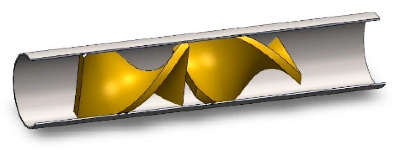
Kenics static mixers, as one of the classic types of static mixers, have the advantages of their unique structure and easy manufacturing. Its structure–function relationship has been extensively studied for many years [11,12,13,14]. The element of the Kenics static mixer is obtained by 180° reversing two ends of a metal blade. As shown in Figure 1, when placed in a circular tube, two elements with different rotational directions need to be placed one by one, intersecting. Mixing the fluid in the Kenics static mixer is accomplished by continuously being split and reorganized by the crossover in the axial flow [15,16,17]. The effectiveness of mixing and the resulting pressure drop depends on the specific geometric parameters of the Kenics static mixer, including the pitch, thickness, and twist angle for each mass transfer element [18,19,20].

In the current state of the art, modifications to standard Kenics static mixers include drilling holes on the blades [21,22], inserting columnar bodies [23], changing the aspect ratio of adjacent elements within a tube [24,25], changing the number of blades [26,27], and stacking multiple Kenics static mixers into the tube [28]. We summarize the thinking behind these modification to the Kenics static mixer and found that they were mainly through “hard additions” to the appearance of the Kenics static mixer. These artworks sought whether this new structure had an enhanced effect on the flow field disturbance by adding an additional structure, which is essentially a departure from the study of how the Kenics static mixer itself interacts with fluid flow.

In contrast to these works, we noticed that standard Kenics static mixers are designed to have a symmetric structure by default. However, how this symmetric structure affects the modification in the axial fluid flow has not been investigated. We believe that the effect of this symmetrical structure is the fundamental reason why Kenics static mixers affect fluid mixing so well.

In order to study the symmetrical structure of the Kenics static mixer itself from the viewpoint of its influence on the fluid flow, we introduced the eccentricity factor $\gamma$, which changes the center position of elements at a twist angle 90°. This paper set heat transfer studies as the background and chose thermal–hydraulic performance factor η as an examination between the heat transfer performance and the pressure drop of different structures. Statistical correlations between the relative Nusselt number and the relative friction factor were proposed with the eccentricity factor, aspect ratio, and Reynolds number by using Latin hypercube sampling with Partial least squares regression (LHS-PLS). To further elucidate the effect of eccentricity on fluid, we simultaneously compared the results of LHS-PLS with the univariate analysis and analyzed two non-standard Kenics static mixers with the introduction of an eccentricity factor using flow field simulation.

2. Materials and Methods

2.1. Design of Numerical Experiments

Latin hypercube sampling with Partial least squares regression (LHS-PLS) is a novel design of experiments that can be used to study the influence of predictor variables on response variables in a broader space [29]. In this method, Latin hypercube sampling is a random sampling method that uses as few points as possible to sample uniformly in the variable space [30], and Partial least squares regression is used to regress between the predictor variables ($AR, Re, \gamma$) and the response variables ($Nu/N{u}_0$, $\lambda /{\lambda }_0$) due to its powerful extraction of the information in the data [31].

Due to introducing a new structural parameter, there may be an unknown interaction between the eccentricity factor and the Aspect ratio (AR). In order to eliminate this interaction, we chose LHS-PLS to study the structure–function relationship of this non-standard Kenics static mixer. LHS results for 20 design points were obtained using Python. The sample set was simulated using OpenFoam v6.0 (The OpenFOAM Foundation Ltd, London, United Kingdom) by the OpenFOAM Foundation Ltd in London, United Kingdom, and the simulation results were regressed in the PLS module of Origin Pro.

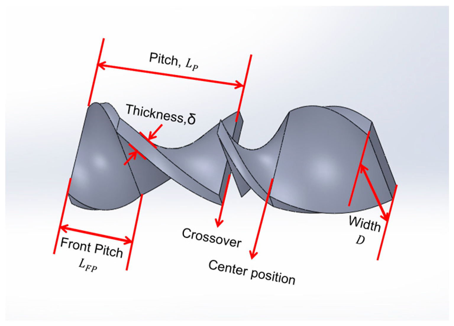
Figure 2 is a schematic diagram to indicate the structure of the mixer and corresponding geometric parameters, and the position of the Kenics static mixer rotated by 90° is defined as the center position. Eccentricity factor $\gamma$ represents the ratio of the front pitch’s length ($L_{FP}$) to the total length ($L_P$) in a unit, as the Equation (1).

$$\gamma =\frac{L_{FP}}{L_P}$$

(1)

The Reynolds number, characterizing the relative influence of inertial and viscous forces, can be calculated by the following Equation:

$$Re=\frac{\rho u_{m}D}{\mu }$$

(2)

The average convective heat transfer coefficient can be calculated as:

$$h_m=\frac{\dot{q}}{T_w-T_m}$$

(3)

The average wall temperature and the average fluid temperature in the full development stage are $T_w$ and $T_m$, respectively. The Nusselt number, which characterizes the strength of convective heat transfer, is defined as:

$$Nu=\frac{h_{m}D}{\lambda }$$

(4)

The whole tube friction factor is defined as:

$$\lambda =\frac{\Delta P}{\left(1/2\rho u^2\right)\left(L_t/D\right)}$$

(5)

The Aspect ratio of the insert is defined as:

$$AR=\frac{L_P}{D}$$

(6)

The thermal–hydraulic performance factor η is defined as Equation (7), where $N{u}_0$ and ${\lambda }_0$ represent the Nusselt number and friction factor of the plain tube, respectively. According to the definition of η, this factor takes into account both the aspects of heat transfer efficiency and resistance characteristics. Thus, we chose the thermal-hydraulic performance factor η as the index of heat transfer performance.

$$\eta =\frac{\left(Nu/N{u}_0\right)}{{\left(\lambda /{\lambda }_0\right)}^{1/3}}$$

(7)

The range of Geometric parameters are shown in

Table 1. Geometric Parameters of modified Kenics static mixer with an Eccentricity factor $\gamma$.

Parameter	Range
Eccentricity factor, $\gamma$	0.25–0.75
Reynolds number, $Re$	3000–13000
Insert width, $D$ (m)	0.002–0.010
Aspect ratio, $AR$	1.0–3.0
Insert thickness, $\delta$ (m)	0.002
Twist angle, $\theta$ (deg)	180

, and the sample set and numerical simulation are shown in the

Table A1. Sample set and numerical simulation of Design Points sampled by Latin hypercube sampling.

No.	AR	D, m	Re	γ	Nu	Nu0	λ	λ0	η
DP1	2.83	0.0069	12665	0.73	474.0	96.9	20.523	0.029	0.591
DP2	2.67	0.0032	6446	0.49	260.6	56.4	6.159	0.036	0.995
DP3	2.33	0.0039	7909	0.32	232.8	66.5	2.540	0.034	0.956
DP4	1.00	0.0040	4000	0.52	239.1	38.5	13.710	0.041	1.211
DP5	1.50	0.0076	5000	0.48	194.2	46.1	3.533	0.039	1.189
DP6	2.22	0.0046	6149	0.74	217.2	54.3	2.977	0.036	1.114
DP7	1.19	0.0083	8692	0.54	354.2	71.7	6.281	0.033	0.972
DP8	1.76	0.0090	5441	0.41	177.0	49.3	2.320	0.038	1.132
DP9	1.11	0.0068	8820	0.58	404.4	72.5	9.049	0.033	0.967
DP10	2.30	0.0043	3551	0.26	131.0	35.0	2.689	0.043	1.320
DP11	2.69	0.0057	9955	0.33	256.3	79.9	1.683	0.031	0.944
DP12	1.43	0.0046	6624	0.72	290.1	57.7	3.041	0.035	1.361
DP13	1.08	0.0095	12712	0.63	468.4	97.2	53.494	0.029	0.422
DP14	2.66	0.0027	3817	0.33	105.6	37.1	1.450	0.042	1.197
DP15	2.38	0.0059	11049	0.28	264.7	86.9	0.166	0.031	1.895
DP16	2.21	0.0093	3671	0.27	125.6	36.0	2.080	0.043	1.324
DP17	1.28	0.0057	10761	0.48	427.4	85.0	7.181	0.031	0.895
DP18	1.70	0.0090	12225	0.51	320.4	94.2	2.144	0.030	0.879
DP19	2.09	0.0070	7616	0.32	201.8	64.5	1.823	0.034	0.964
DP20	1.07	0.0067	5826	0.73	298.7	52.1	10.148	0.037	1.082

of Appendix A.

2.2. Computational Fluid Dynamics

The impact of turbulence was obtained using a choice of momentum and energy Realizable k-ω-realizable equations. The details of these equations are shown in

Table A2. Details of momentum and energy Realizable k-ω-realizable equations.

Names	Equations
Equation of continuity	$\frac{\partial }{\partial x_i}\left(\rho u_i\right)=0$
Equation of momentum	$\frac{\partial }{\partial x_j}\left(\rho u_j{u}_i\right)=-\frac{\partial P}{\partial x_i}+\frac{\partial {\tau }_{ij}}{\partial x_j}$
Equation of energy	$\frac{\partial }{\partial x_j}\left[\rho u_j\left(\mathsf{\theta }+\frac{1}{2}{u}_i{u}_i\right)\right]=\frac{\partial }{\partial x_j}\left(u_i{\tau }_{ij}\right)+\frac{\partial }{\partial x_j}\left(k\frac{\partial T}{\partial x_j}\right)$
Equation of turbulent kinetic energy	$\frac{\partial }{\partial x_i}\left(\rho K{u}_i\right)=\frac{\partial }{\partial x_j}\left[\left(\mu +{\mu }_T\right)\frac{\partial K}{\partial x_j}\right]+2{\mu }_T{S}_{ij}{S}_{ij}-\rho e$
Equation of turbulence dissipation rate of kinetic energy	$\begin{array}{l}\frac{\partial }{\partial x_i}\left(\rho e{u}_i\right)=\frac{\partial }{\partial x_j}\left[\left(\mu +\frac{{\mu }_T}{1.3}\right)\frac{\partial e}{\partial x_j}\right]+\\ \rho e\sqrt{2S_{ij}{S}_{ij}}\max \left[0.43,\frac{\frac{2S_{ij}{S}_{ij}K}{e}}{5+\frac{2S_{ij}{S}_{ij}K}{e}}\right]-1.9\rho \frac{e^2}{K+\sqrt{\frac{\mu }{\rho }}e}\end{array}$
Equation of turbulent viscosity	${\mu }_T=\rho \frac{K^2}{e}\left[\frac{1}{4.04+2.45\frac{K}{e}\cos \left[0.33{\cos }^{-1}\left(\frac{2.45S_{ij}{S}_{jk}{S}_{ki}}{{\left(S_{ij}{S}_{ij}\right)}^{0.67}}\right)\right]}\right]$
Equation of tensor of the strain rate	$S_{ij}=0.5\left(\frac{\partial {\overline{u}}_i}{\partial x_j}+\frac{\partial u_j}{\partial x_i}\right)$

. Based on this, the second-order upwind scheme was used to discretize each conservation relation. In the numerical simulation of fluid flow, coupling of velocity and pressure is required. We established the SIMPLEC algorithm for this purpose [32]. Moreover, the magnitude of the wall and energy Prandtl number was equal to 0.05. This value provides the most agreement between the numerical results and the experimental data for the present study. The acceptable residual for the continuity momentum energy and k-ω-realizable equations are lower than 10⁻³, 10⁻⁴, 10⁻⁶, and 10⁻⁵, respectively. Each case needs at least 500 iterations to achieve convergence.

No-slip boundary conditions were used for the tube wall and the ’inserts’ surface. A constant heat flux of 10,000 w/m² was applied to the tube wall, and since the temperature rise was not significant, the changes in density and viscosity due to temperature were negligible. In Meng [12], it has been demonstrated that the mass and heat transfer properties are stabilized after passing through the 12 section cell. To reduce the computational effort while the effect of geometric parameters is being examined, after the flow field has been fully developed, periodic boundary conditions are used at the inlet and outlet.

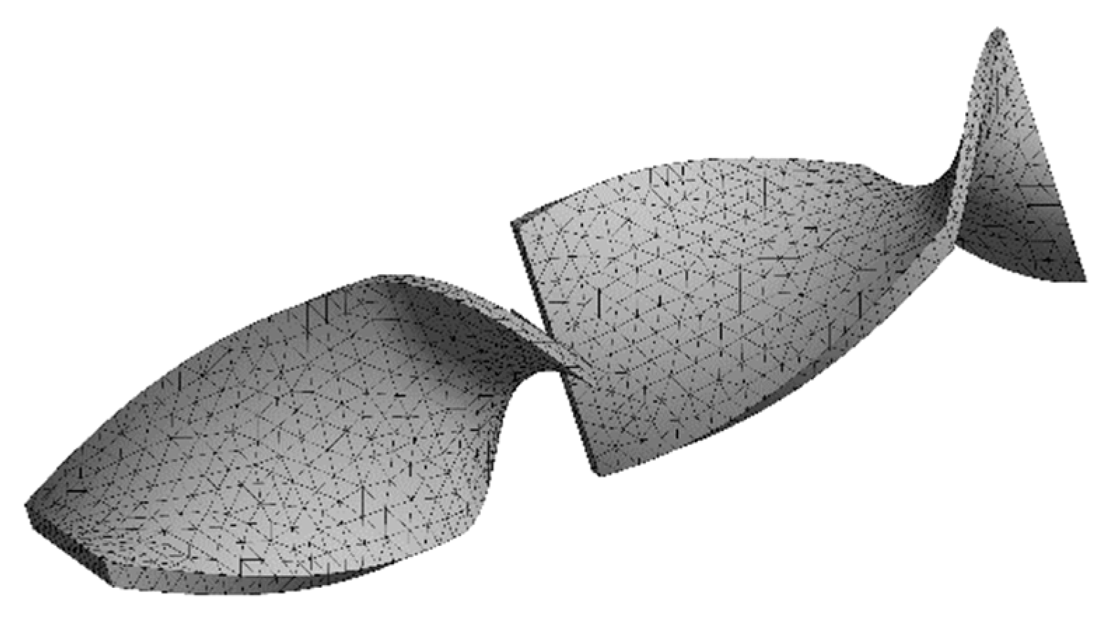
As shown in Figure 3, we generated a 3D tetrahedral mesh with an expansion layer added to the tube walls and inserts to bring the elements into contact with the inside of the tube walls. The layer ensured that there were no gaps between the inserts and the wall. We used tetrahedral elements to generate meshes on the Kenics static mixer. In addition, for a more accurate simulation of the boundary layer, the meshes close to the solid surface were decomposed into smaller meshes in the regions with a higher y⁺ to make it lower.

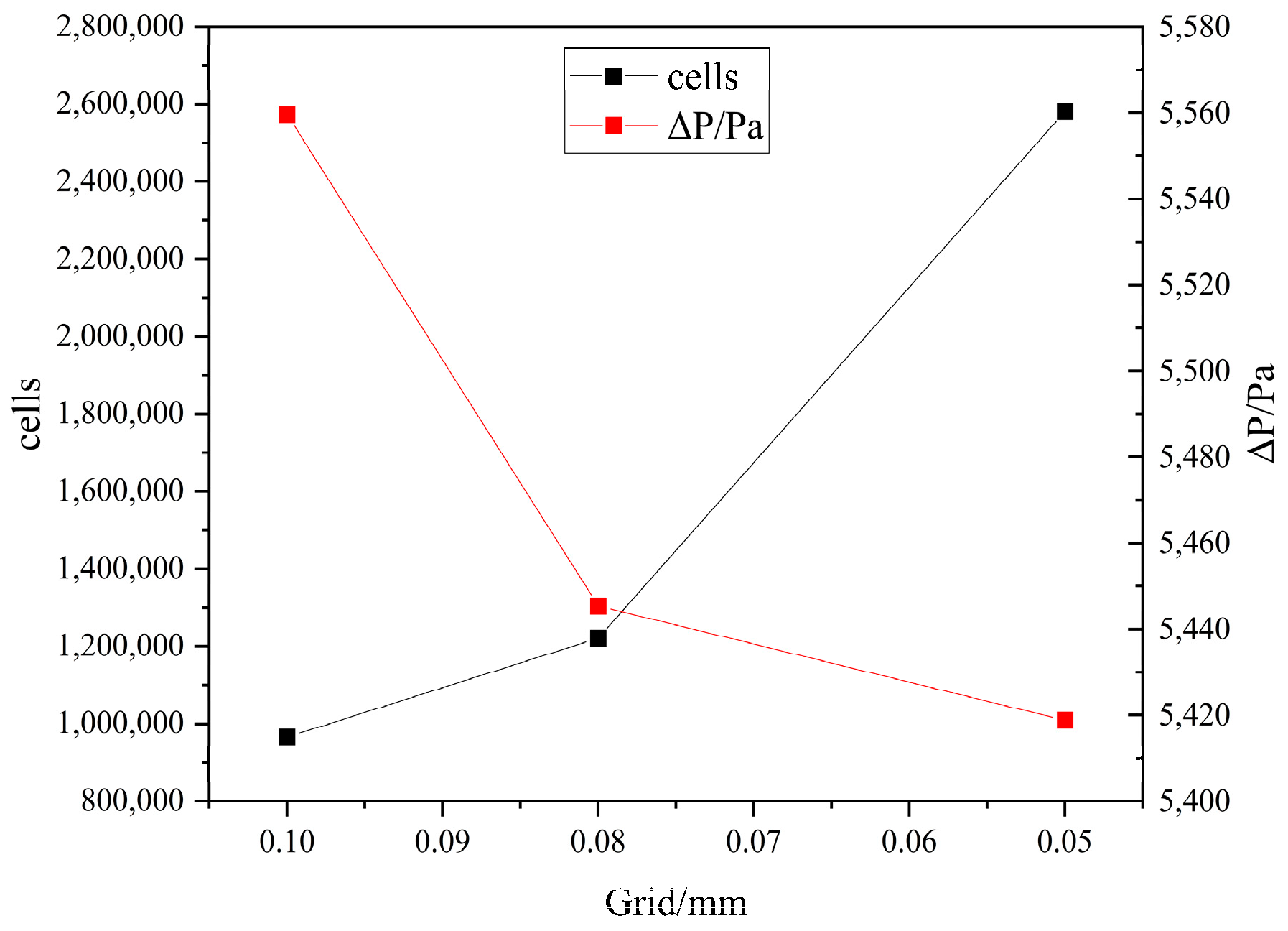
For verifying the independence of the meshes, three different meshes were generated for $Re=8000$ and $AR=2.0$, with element sizes of 0.10 mm, 0.08 mm, and 0.05 mm, respectively. As shown in Figure 4, the pressure drop decreased by 0.5%, and the number of meshes increased by 111.4% as the size decreased from 0.08 mm to 0.05 mm. In order to balance the computational accuracy and computational resources, we choose a 0.08 mm mesh to build the model.

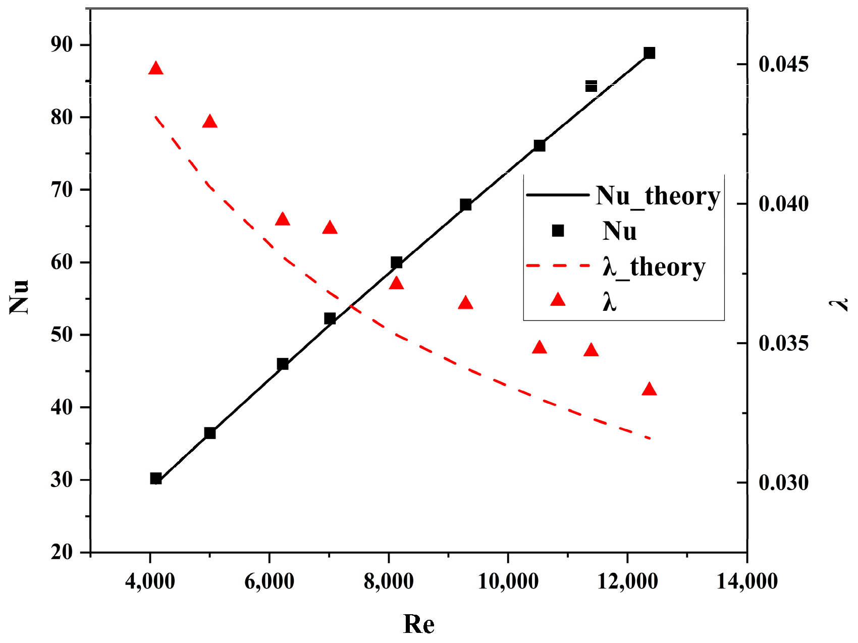
Theoretical values of Nusselt number Equation (8) and friction factor Equation (9) obtained from Gnielinski [33] and Filonenko [34] correlations were applied to validate heat transfer performances and flow in the plain tube, respectively. As shown in Figure 5, good agreements were obtained as the deviations between the simulative and theoretical values, which were 2.1% for the Nusselt number and 5.2% for the friction factor.

$$N{u}_0=0.012\left(R{e}^{0.87}-280\right)P{r}^{0.4}$$

(8)

$${\lambda }_0={\left(1.82\lg \left(Re\right)-1.64\right)}^{-2}$$

(9)

3. Results and Discussion

3.1. Explanation of PLS Model

The numerical simulation result data were put into the PLS model as response variables. The fitting results could be obtained by regressing the predictor variables on the response variables in the latent space.

In the PLS model, we assumed that the system under study was actually influenced by a combination of variables into latent variables; the predictor variables were linearly combined into a latent variable t, the response variables were linearly combined into a latent variable v, and the latent variables t and v were tensored into a latent space. Therefore, the interpretation of the PLS fit results needs to be performed in the latent space.

We regarded the variance of the data as the information contained in the data. Usually, a pair of latent variables t and v are called components, which extract information from the original variables in turn, and different components have different abilities to extract information. Cross Validation (CV) is a practical and reliable method to determine the number of components (latent variable pairs) [35]. In this study, two components were determined to be sufficient to extract all the information by CV, as shown in

Table 2. Cross validation of the PLS model for Kenics static mixers with an eccentricity factor.

Number of Components	Variance Explained for X Effects (%)	Cumulative X Variance (%)	Variance Explained for Y Responses (%)	Cumulative Y Variance (%)
1	53.85	53.85	56.86	56.86
2	31.44	85.29	10.72	67.58

.

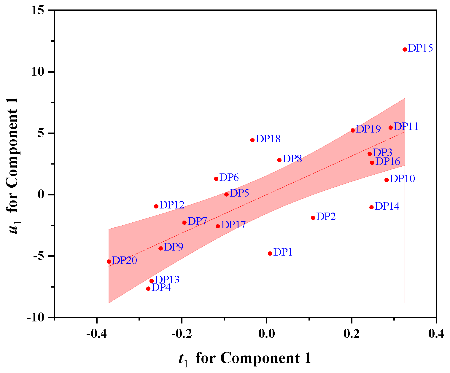
It can be seen that component 1 extracted 56.86% of the information in the response variable Y. Therefore, we only needed to focus on the relationship between latent variables v and t in the two-dimensional latent space spanned by component 1, as shown in Figure 6.

Figure 6 shows the latent space for component 1, with the latent variable t, consisting of the predictor variable $AR, Re, \gamma$ as the horizontal coordinate. The latent variable v, consisting of the response variable $Nu/N{u}_0$ and $\lambda /{\lambda }_0$ as the vertical coordinate, and the 20 design points were projected into this latent variable space. The red region is the 95% confidence interval, and the regression errors for all points were within 10%, which indicates that the PLS model could be used to analyze the design of a non-standard Kenics static mixer with the introduction of an eccentricity factor $\gamma$.

The numerical simulation results were put into the PLS as response variables, and the fitting results were obtained by regressing the $AR, Re, \gamma$ and $Nu/N{u}_0$ and $\lambda /{\lambda }_0$ in the latent space as follows:

$$\lg \left(\frac{Nu}{N{u}_0}\right)-0.4\cdot \lg \left(Pr\right)=-0.285\cdot \lg \left(AR\right)-0.366\cdot \lg \left(Re\right)+0.258\cdot \lg \left(\gamma \right)+1.93$$

(10)

$$\lg \left(\frac{\lambda }{{\lambda }_0}\right)=-1.22\cdot \lg \left(AR\right)+0.293\cdot \lg \left(Re\right)+1.47\cdot \lg \left(\gamma \right)+1.72$$

(11)

Transforming the fit results, we obtained the statistical correlations (12) and (13).

$$\frac{Nu}{N{u}_0}=85.11\cdot A{R}^{-0.285}R{e}^{-0.366}{\gamma }^{0.258}P{r}^{0.4}$$

(12)

$$\frac{\lambda }{{\lambda }_0}=52.48\cdot A{R}^{-1.22}R{e}^{0.293}{\gamma }^{1.47}$$

(13)

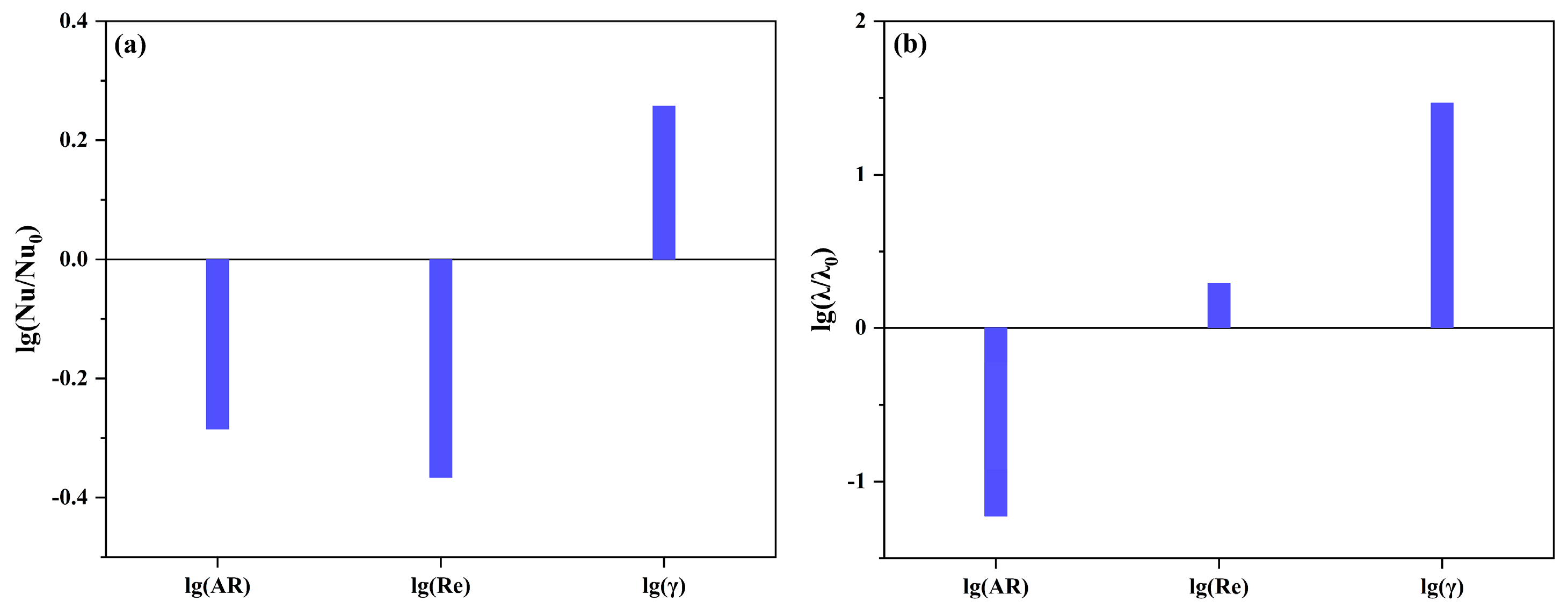
The PLS model with the introduction of the eccentricity factor was analyzed using regression coefficient plots and variable importance plots. As shown in Figure 7, the regression coefficients between the $AR, Re, \gamma$ and the response variable $Nu/N{u}_0$ were −0.285, −0.366, and 0.258, respectively, indicating that $AR, Re$ were negatively correlated with the $Nu/N{u}_0$; meanwhile, $\gamma$ was positively correlated with it. All three variables had a strong effect on the relative Nusselt number.

For the relative friction factor, the coefficient of the variable $AR$ was –1.22, which was strong negative correlated with $\lambda /{\lambda }_0$, while the coefficient of the variable $Re$ was 0.293, which was weakly positively correlated with $\lambda /{\lambda }_0$. The variable $\gamma$ was 1.47, which indicated a strong positive correlation with the relative friction factor.

Overall, the aspect ratio, which characterizes the structural properties of the Kenics static mixer, had the largest regression coefficient for heat transfer and pressure drop. The introduction of the eccentricity factor also had a significant effect on both response variables, which indicated that the fluid was affected by the symmetric structure during the fluid flow through elements, and this effect was neglected in previous studies.

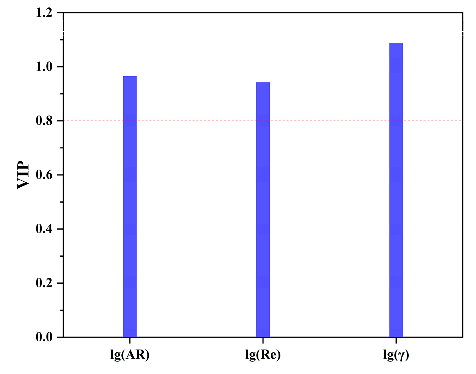
Figure 8 shows the projection of the three ’variables’ importance. It can be seen that, as with the analysis of the regression coefficients, the effect of the aspect ratio $AR$ and the eccentricity factor $\gamma$ on the heat transfer performance was more significant. This is due to the fact that in the iterative process of stepwise regression, the data fluctuations of $AR$ and $\gamma$ had a more significant influence on the response variable $Nu/N{u}_0$ and $\lambda /{\lambda }_0$, relative to the Reynolds number $Re$, which resulted in the situation that during the process of extracting information, the aspect ratio and the eccentricity factor were more able to explain the degree of variation of the response variable in the variation of the structural parameters. Therefore, $AR$ and $\gamma$ had a higher weight in the statistical index of the importance of the response variable.

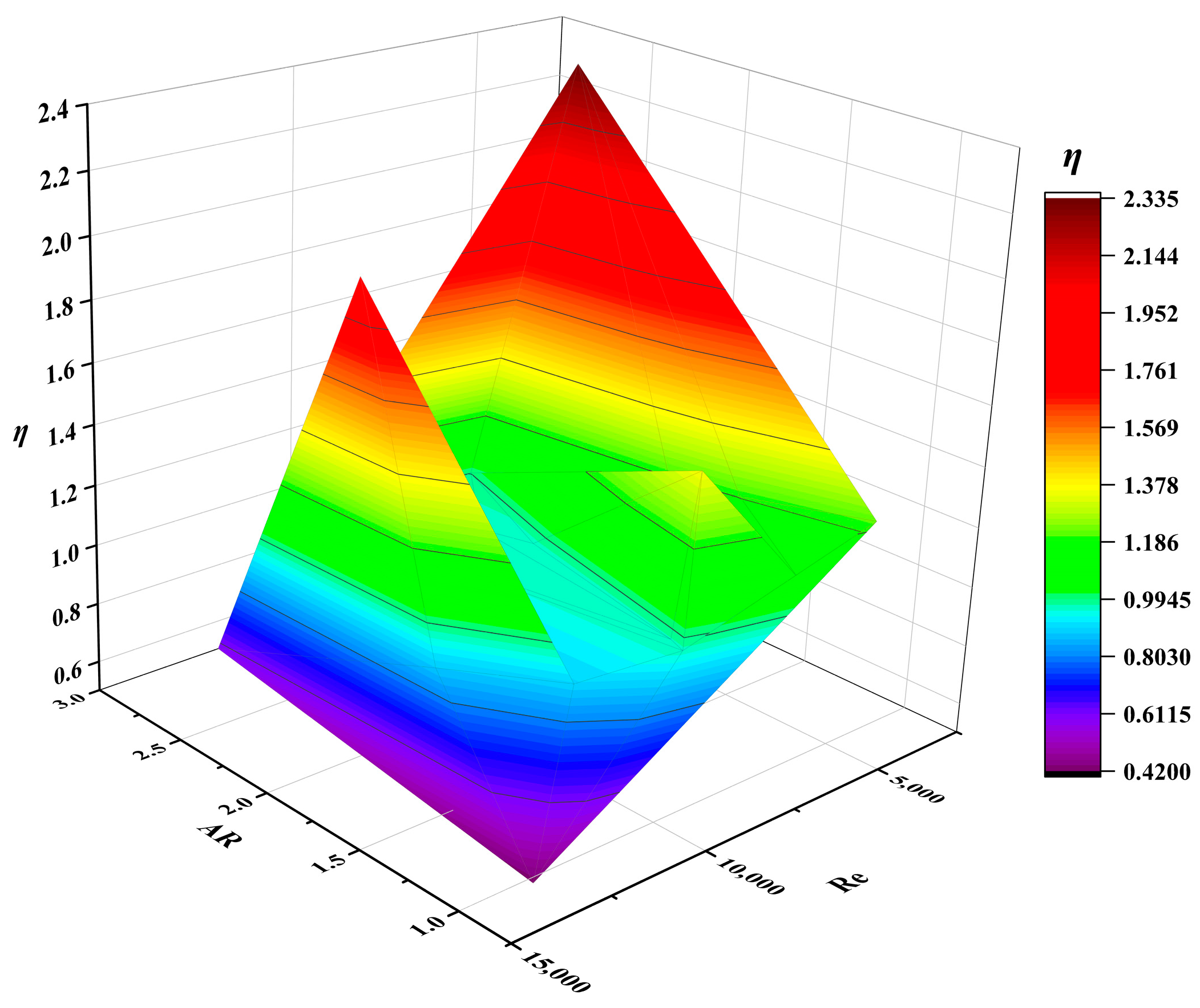
The 3D contour plots of the thermal–hydraulic performance factor η for each physical model under the introduction of the eccentricity factor are shown in Figure 9. The higher the value of η, the better the heat transfer performance. At $AR=2.38$ and $Re=\mathrm{11,049}$, η reached maximum at 1.895.

In Figure 9, three of the 20 design points were the extreme values of the thermal-hydraulic performance factor in the sample space, namely DP12, DP14, and DP15. However, the conventional symmetric structure of the Kenics static mixer, where $\eta$ increases with decreasing $Re$ and increasing $AR$, did not have an extreme value point [36,37], as could be derived from the empirical correlations. To further investigate the effect of the eccentricity factor $\gamma$ on the dimensionless number $Nu, \lambda$, and the thermal–hydraulic performance factor η, we selected two design conditions for a univariate analysis.

3.2. Univariate Analysis

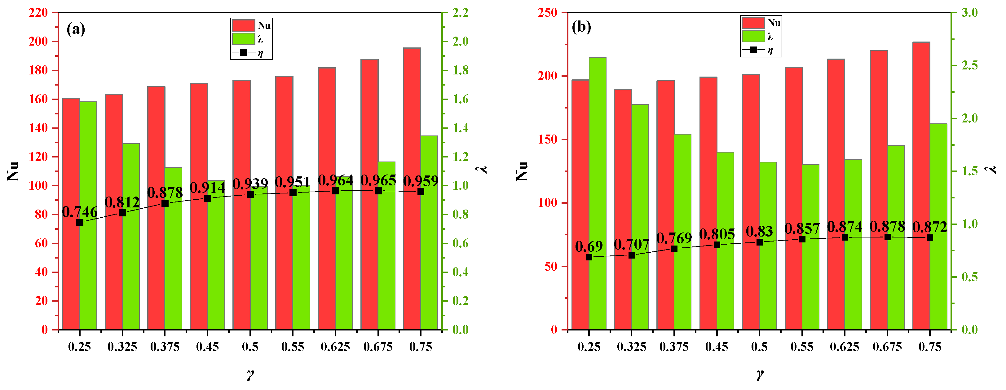
In the one-way analysis, we modified the centrosymmetric position under the two design points and investigated the $Nu, \lambda ,$ and $\eta$ by only changing $\gamma$ from 0.25 to 0.75. Data is shown in

Table A3. Data of two Design points changing the centro-symmetric: (a) $Ar=2.0, Re=7000$; (b) $Ar=1.5, Re=8000$.

(a)	AR	D, m	Re	γ	Nu	Nu0	λ	λ0	η
	2.00	0.0050	7000	0.25	160.4	60.3	1.582	0.0346	0.744
	2.00	0.0050	7000	0.325	163.2	60.3	1.291	0.0346	0.810
	2.00	0.0050	7000	0.375	168.8	60.3	1.128	0.0346	0.876
	2.00	0.0050	7000	0.45	170.7	60.3	1.037	0.0346	0.911
	2.00	0.0050	7000	0.5	173.0	60.3	0.993	0.0346	0.937
	2.00	0.0050	7000	0.55	175.7	60.3	1.003	0.0346	0.949
	2.00	0.0050	7000	0.625	181.7	60.3	1.064	0.0346	0.962
	2.00	0.0050	7000	0.675	187.5	60.3	1.166	0.0346	0.963
	2.00	0.0050	7000	0.75	195.5	60.3	1.346	0.0346	0.957
(b)	AR	D, m	Re	γ	Nu	Nu0	λ	λ0	η
	1.50	0.0080	8000	0.25	197.0	67.1	2.578	0.0335	0.690
	1.50	0.0080	8000	0.325	189.5	67.1	2.131	0.0335	0.707
(b)	AR	D, m	Re	γ	Nu	Nu0	λ	λ0	η
	1.50	0.0080	8000	0.375	196.4	67.1	1.850	0.0335	0.768
	1.50	0.0080	8000	0.45	199.2	67.1	1.680	0.0335	0.805
	1.50	0.0080	8000	0.5	201.5	67.1	1.587	0.0335	0.830
	1.50	0.0080	8000	0.55	207.0	67.1	1.563	0.0335	0.857
	1.50	0.0080	8000	0.625	213.4	67.1	1.614	0.0335	0.874
	1.50	0.0080	8000	0.675	220.0	67.1	1.744	0.0335	0.878
	1.50	0.0080	8000	0.75	226.7	67.1	1.949	0.0335	0.872

.

In the two design points of Figure 10, we can see that the $Nu$ represented by the red column increased with the increase of the eccentricity factor $\gamma$, which is consistent with the positive regression coefficient of $\gamma$ on $Nu/N{u}_0$ in the PLS model. The friction factor $\lambda$ represented by the green column tended to decrease and then increase with the eccentricity factor$\gamma$. The friction factor at $\gamma =0.5$ was the smallest, which corresponds to the classical centrosymmetric Kenics static mixer structure.

We analyzed the similarities and differences between the PLS model and the univariate analysis with the introduction of the eccentricity factor.

(1) The total information extraction ratio of the model for X and Y was 85.29% and 67.58%, which indicates that the LHS-PLS is applicable to the Kenich static mixer with the introduction of eccentricity factor but that the limited fitting capability causes some information loss. By analyzing the study cases in which PLS was applied, we suggest that although the study subjects are all Kenics static mixers, the underlying logic of the fluid exerted by Kenics static mixers with extreme eccentricity factors and those with near-centrosymmetric structures may have changed in the 20 samples after the introduction of eccentricity factors. This is the reason why the results of PLS were not consistent with those of the univariate analysis. Considered from a different perspective, this is evidence that the “centrosymmetric structure” in the design of the Kenics static mixer was not only due to mechanical constraints, but also due to the rationality of the structure itself, which is why the friction factor was minimal at $\gamma =0.5$ in the univariate analysis. This possible variation of the underlying logic is further explained in Section 3.3 from the view of the flow field.

(2) In the CFD simulation of the Kenics static mixer with a changing centrosymmetric position, we found that compared to the classical one, the combination of variables of some design points will get an abnormal $Nu$ and $\lambda$; the points constituted exceeded the 95% confidence limits of the latent variable space, i.e., the confidence ellipse with DP14 and DP15 in Figure 6, and these two points happened to be the 20 sample points with the largest coefficients of thermal–hydraulic performance. This proves that the underlying logic of the Kenics static mixer with an asymmetric structure became more complex, ensuring the reliability of the CFD simulation.

(3) In the PLS model, we conclude that the regression coefficient of the eccentricity factor $\gamma$ on $\lambda /{\lambda }_0$ was 1.47, where this was different from the results of the univariate analysis. In the univariate analysis in Figure 10, we found that the friction factor increased when the centrosymmetric position moved in the direction of the two extremes, i.e., $\gamma \to 0.25$ or $0.75$. Since the regression of PLS on the variables only yields one coefficient, more consideration was given to the degree of variance of the variables in the fitting process, which reflects the relationship between the variance and the responses. This was the reason why the results of the regression coefficients analysis in the PLS model differed from those of the univariate analysis; if the degree of deviation from the center of the symmetric position was taken into account in the univariate analysis, i.e., $\left|\gamma -0.5\right|$, the results of the univariate analysis corresponded to the regression coefficients of the PLS model. The results of the univariate analysis also explained the decrease in the information extraction rate of the PLS model.

In this section, we modified the structure of the standard Kenics static mixer to study the guide effect of the Kenics static mixer on the fluid by changing its centrosymmetric position. In our study, we found that the information extraction ability of the LHS-PLS for 20 sample points was reduced after the introduction of the eccentricity factor. By comparing the results with those of the univariate analysis, we attribute this discrepancy to the fact that some non-standard Kenics static mixers with extreme asymmetric structures differ in their effect on fluid guidance from classical ones. This conclusion corroborates that the default centrosymmetric structure of the Kenics static mixer is the one that has a direct impact on mixing and heat transfer during fluid flow. When studying the structure of Kenics static mixer, it is not reasonable to consider only the cutting effect of the crossover on the fluid and ignore the pressure drop and mixing caused by the rotation of the fluid along the course. In addition, in the univariate analysis, changing only the centrosymmetric position, we found that the default structure did have the lowest pressure drop, but the backward eccentric Kenics static mixer had a higher Nusselt number and thermal–hydraulic performance factor, for which we analyzed the differences in the flow field at different design points in Section 3.3.

3.3. Analysis through Flow Field Simulation

Through flow field simulation, we investigated the mechanism that affects the heat transfer efficiency by describing the fluid flow in the case of an asymmetric Kenics static mixer structure. The mechanism by which the Kenics static mixer triggers fluid rotation to generate vortices, and thus affects mixing and heat transfer, has been discussed in literature [13,25,38,39]. With the introduction of the eccentricity factor, the generation of vortices remains the primary factor for enhanced heat transfer. After the introduction of vortices, firstly, we should be more concerned with the extent to which the velocity boundary layer and the thermal boundary layer were effectively thinned. Secondly, the asymmetric position of the elements changed the flow path of the fluid. The fluid was distorted differently during the guideline process, which affected the impact of the fluid on the boundary layer and the formation of vortices, further affecting the heat transfer performance.

To further analyze the vortex generation and dissipation, we continued from the radial section and axial interface.

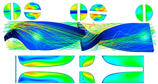
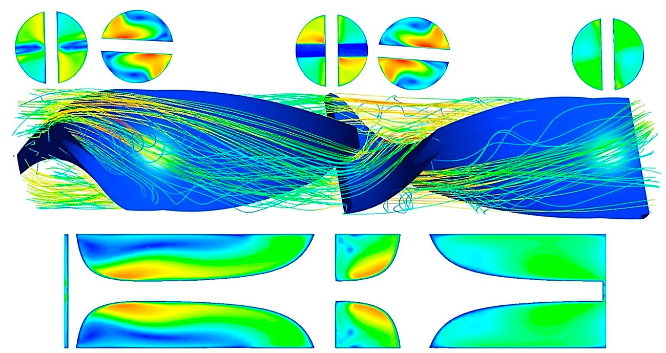
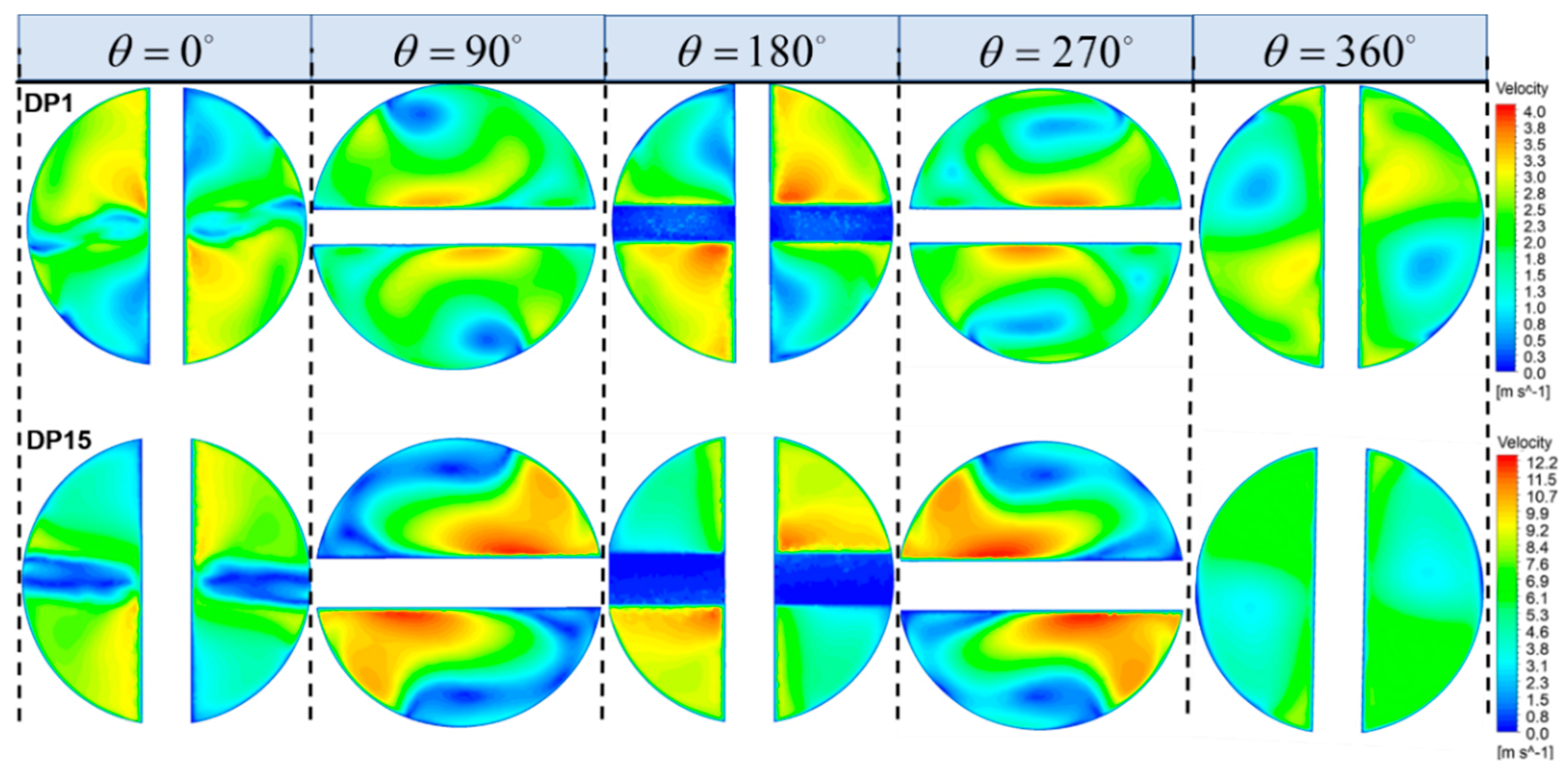
Figure 11 shows the velocity field of DP7 and DP15, and each design point contained two adjacent cells that were twisted by a total of 360°, where the inlet $\theta =0^{\circ }$, the center of the first element $\theta ={90}^{\circ }$, the crossover $\theta ={180}^{\circ }$, the center of the second element $\theta ={270}^{\circ },$ and the exit $\theta ={360}^{\circ }$. We found that a significant vortex was formed in the velocity field of both DP7 and DP15 at $\theta ={90}^{\circ }$ with $\theta ={270}^{\circ }$, and this stronger velocity gradient gradually weakened at the crossover, i.e., $\theta ={180}^{\circ }$. This indicates that the vortices formed during the fluid being guided by the components were relatively intense at the center of the cell, and this vortex was the main reason for the thinning of the thermal and velocity boundary layers. Comparing the two design points, we found that the degree of the vortex was greater in DP15 than in DP7, which had a higher thermal–hydraulic performance factor, and the former was therefore due to this stronger vortex. It makes sense to introduce an eccentricity factor in the study of Kenics static mixers.

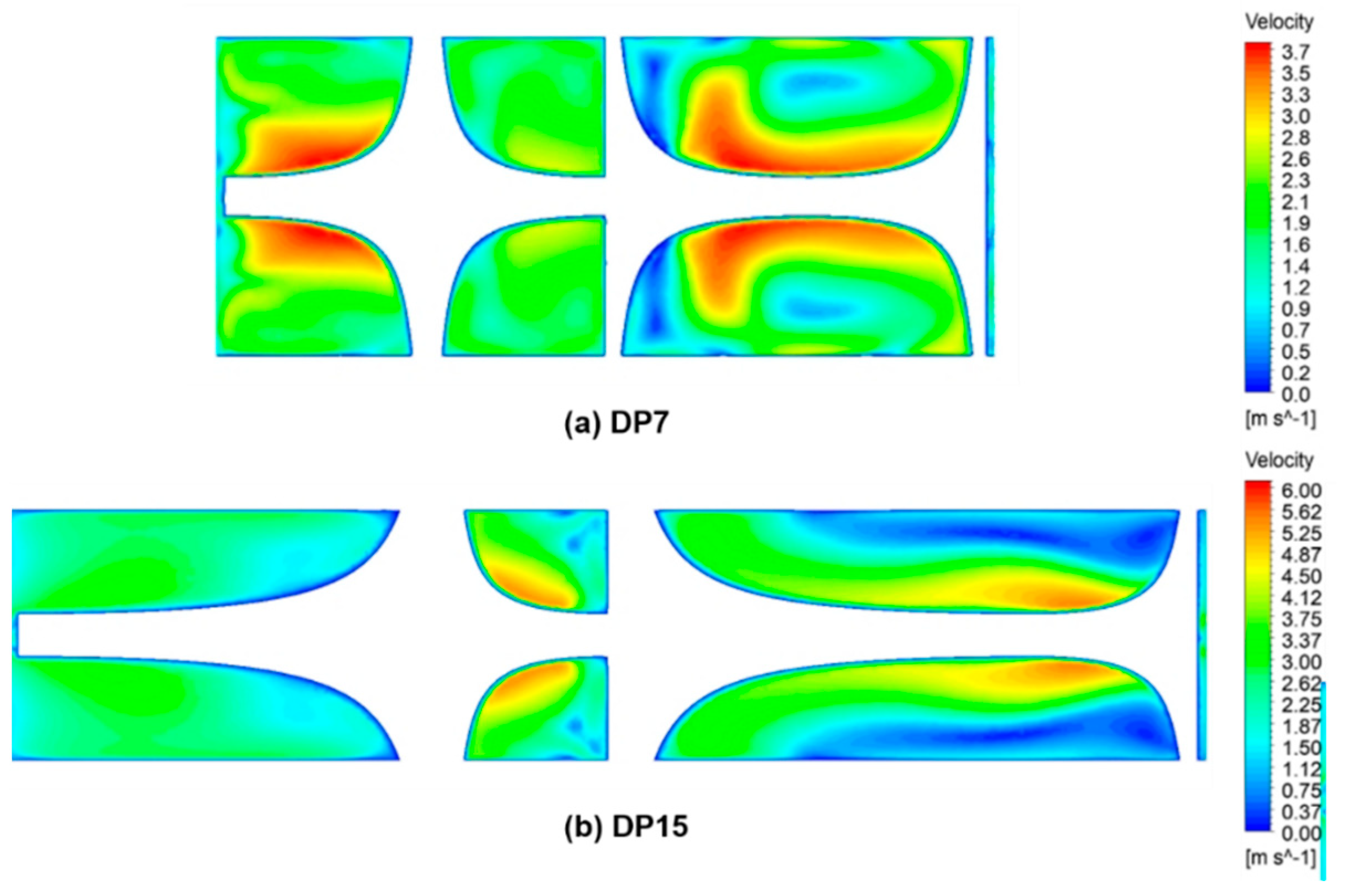
Figure 12 shows the velocity fields of the two adjacent elements’ axial cross-sections at the two design points of DP7 and DP15. Comparing Figure 12a,b, it is obvious that the pattern of fluid flow changed due to the introduction of the eccentricity factor. DP15 with a smaller eccentricity factor $\gamma$ had a stronger velocity gradient at the axial interface and a greater degree of fluid rotation. The flow simulation showed that the twisting of the fluid was more intense in the part near the inlet section, due to the change of the center position, which corresponds to an element with a smaller $AR$. Naturally the larger is the $AR,$ the smaller the pressure drop and the better the heat transfer performance. This is reflected in the backward part of DP15, where the velocity boundary layer was thin, and the velocity gradient was small. Comparing with DP7, we realize that when the center of the Kenics static mixer was changed, it was equivalent to connecting two Kenics static mixers with the same diameter but different aspect ratios at $\theta ={90}^{\circ }$. This connection resulted in the formation of vortices more quickly when the fluid struck the element surface due to the large distortion of the insert with a smaller $AR$, but with a cost of a higher pressure drop. This velocity gradient could be released backwards on the side with a larger $AR$, and the number of crossovers during per element length was reduced, which reduced the pressure drop to some extent. This was finally reflected in the univariate analysis, where the pressure drop showed a trend of decreasing and then increasing with the eccentricity factor $\gamma$ increased.

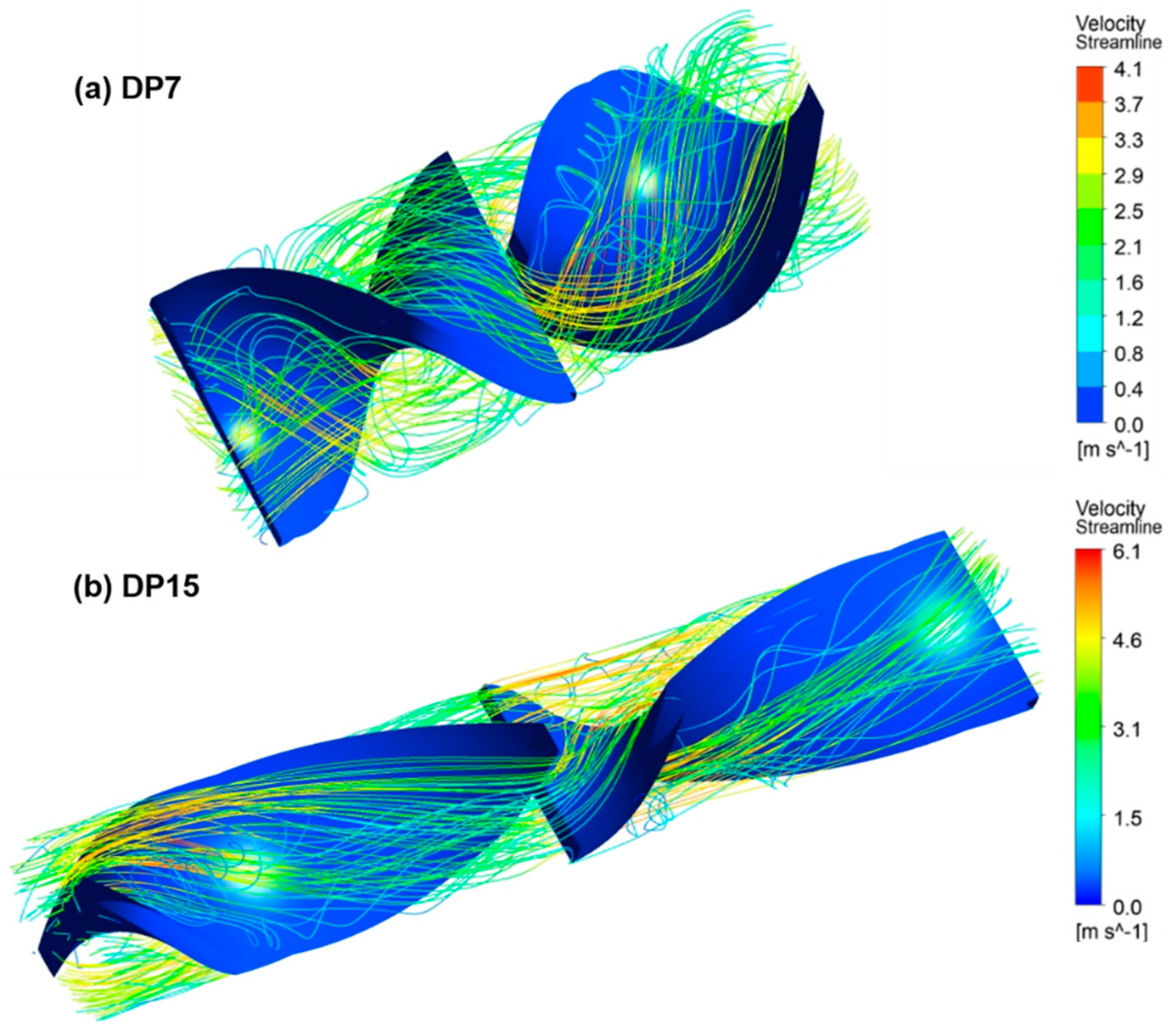
Figure 13 shows the streamline after combining two adjacent elements of DP7 and DP15, and it can be seen that DP7 with a shorter aspect ratio had a more distorted flow. By analyzing the axial interface, we obtained that the essence of changing the centrosymmetric position was the combination of two elements with different aspect ratios at $\theta ={90}^{\circ }$. Comparing Figure 13a,b, when the fluid entering DP15 passed through the shorter front end, the back mixing was obvious due to the higher torque and the strong strike of the fluid on the wall. This is reflected in the part of Figure 13 where the red flow line intersected with the green flow line, corresponding to a larger velocity gradient. Afterward, this vortex structure continued to move forward with the flow body and wss gradually dissipated backward.

Throughout the process, the vortex generation and dissipation mechanism in the non-standard Kenics static mixer with an eccentricity factor were the same as in the standard Kenics static mixer but to a different extent due to the eccentricity. This happens to be the underlying logic of how the Kenics modify the fluid, but this logic cannot be explored and explained in the standard Kenics static mixer with only a change in the aspect ratio.

The above explanation made in conjunction with the flow field simulation proves what we concluded in Section 3.1 and Section 3.2: when the center of symmetry of the Kenics static mixer is shifted, its mechanism acting on the flow field is changed, which eventually leads to a decrease in the amount of information extracted from the sample set by the PLS model and the difference between the univariate analysis and the PLS model.

In this section, the velocity field of a non-standard Kenics static mixer with the introduction of an eccentricity factor was visualized. Starting from the vortices generated and dissipated by the twisted flow path, this asymmetric structure was studied. The result showed that the nature of the eccentric structure is a combination of two components with different aspect ratios at $\theta ={90}^{\circ }$. This articulation led to a non-standard Kenics static mixer with different combinations having different underlying mechanisms; even though the mechanisms of vortex generation and dissipation were the same, the intensity of generation and the time required for dissipation were different. These explained the differences between the PLS models and the univariate analysis.

4. Conclusions

The standard Kenics static mixer design with its default centrosymmetric structure obviously contains a mechanical limitation and is prior and subjective. How to study this “Deserved Design” and how to get rid of purposeless parameter modification is a new way to think about the design of inserts in fluid flow research.

In order to study how the symmetrical structure of the Kenics static mixer itself impacts the fluid flow, we changed the central center position of elements at twist angle 90° and introduced the eccentricity factor $\gamma$. We applied LHS-PLS to study this non-standard Kenics static mixer. From the fitting results of the PLS model, we observed that the information extraction of PLS was reduced due to the introduction of an eccentricity factor, but the method itself did not fail. It was shown that the eccentricity factor $\gamma$ had a positive effect on the $Nu/N{u}_0$ and $\lambda /{\lambda }_0$, while $AR$ and $Re$ were negative. All three variables were important due to the VIP plot, and $\gamma$ was the most important one. In addition, the introduction of the $\gamma$ caused the extreme value point in the sample set, and we analyzed this phenomenon by comparing the fitted multivariate PLS model with the univariate analysis of the control variables method. It was found that the underlying logic of the Kenics static mixer with an asymmetric structure became more complex, and the default structure did have the lowest pressure drop, but the backward eccentric Kenics static mixer had a higher Nusselt number and thermal–hydraulic performance factor.

For a further exploration of the underlying, we studied two non-standard Kenics static mixers’ flow field simulations. It was found that the nature of the eccentric structure was that two elements with different aspect ratios were being combined at $\theta ={90}^{\circ }.$ This articulation led to non-standard Kenics static mixers with different underlying logic, which finally resulted in the differences between the PLS model and the single factor analysis.

References

- Yarn, K.F.; Hsu, S.P.; Luo, W.J. Microfluidic mixing enhancement using electrokinetic instability under electric field perturbations in a double T-shaped microchannel. Sci. China Ser. G Phys. Mech. Astron. 2009, 52, 602–612. [Google Scholar] [CrossRef]
- Luo, W.-J.; Yarn, K.-F.; Hsu, S.-P. Analysis of Electrokinetic Mixing Using AC Electric Field and Patchwise Surface Heterogeneities. Jpn. J. Appl. Phys. Part Regul. Pap. Brief Commun. Rev. Pap. 2007, 46, 1608. [Google Scholar] [CrossRef]
- Tsukiyama, S.; Takamura, A.; Nakano, M. Liquid-liquid dispersion on mechanical agitation. V. Effect of pre-agitation on colloid mill (author’s transl). Yakugaku Zasshi J. Pharm. Soc. Jpn. 1973, 93, 1131–1137. [Google Scholar] [CrossRef] [Green Version]
- Thakur, R.K.; Vial, C.; Nigam, K.D.P.; Nauman, E.B.; Djelveh, G. Static Mixers in the Process Industries—A Review. Chem. Eng. Res. Des. 2003, 81, 787–826. [Google Scholar] [CrossRef]
- Zheng, N.; Liu, P.; Liu, Z.; Liu, W. Numerical simulation and sensitivity analysis of heat transfer enhancement in a flat heat exchanger tube with discrete inclined ribs. Int. J. Heat Mass Transf. 2017, 112, 509–520. [Google Scholar] [CrossRef]
- Lee, C.Y.; Chang, C.L.; Wang, Y.N.; Fu, L.M. Microfluidic Mixing: A Review. Int. J. Mol. Sci. 2011, 12, 3263–3287. [Google Scholar] [CrossRef] [PubMed] [Green Version]
- Ghanem, A.; Lemenand, T.; Della Valle, D.; Peerhossaini, H. Static mixers: Mechanisms, applications, and characterization methods—A review. Chem. Eng. Res. Des. 2014, 92, 205–228. [Google Scholar] [CrossRef]
- Myers, K.J.; Bakker, A.; Ryan, D. Avoid agitation by selecting static mixers. Chem. Eng. Prog. 1997, 93, 28–38. [Google Scholar]
- Meijer, H.E.H.; Singh, M.K.; Anderson, P.D. On the performance of static mixers: A quantitative comparison. Prog. Polym. Sci. 2012, 37, 1333–1349. [Google Scholar] [CrossRef] [Green Version]
- Cybulski, A.; Werner, K. Static mixers-criteria for applications and selection. Int. Chem. Eng. 1986, 26, 171–180. [Google Scholar]
- Galaktionov, O.; Anderson, P.; Peters, G.; Meijer, H. Analysis and optimization of Kenics static mixers. Int. Polym. Process. 2003, 18, 138–150. [Google Scholar] [CrossRef] [Green Version]
- Meng, H.; Zhu, G.; Yu, Y.; Wang, Z.; Wu, J. The effect of symmetrical perforated holes on the turbulent heat transfer in the static mixer with modified Kenics segments. Int. J. Heat Mass Transf. 2016, 99, 647–659. [Google Scholar] [CrossRef]
- Murasiewicz, H.; Zakrzewska, B. Large Eddy Simulation of turbulent flow and heat transfer in a Kenics static mixer. Chem. Process Eng. 2019, 40, 87–99. [Google Scholar]
- Joshi, P.; Nigam, K.; Nauman, E.B. The Kenics static mixer: New data and proposed correlations. Chem. Eng. J. Biochem. Eng. J. 1995, 59, 265–271. [Google Scholar] [CrossRef]
- Hobbs, D.; Muzzio, F. The Kenics static mixer: A three-dimensional chaotic flow. Chem. Eng. J. 1997, 67, 153–166. [Google Scholar] [CrossRef]
- Hobbs, D.; Muzzio, F. Optimization of a static mixer using dynamical systems techniques. Chem. Eng. J. 1998, 53, 3199–3213. [Google Scholar] [CrossRef]
- Hobbs, D.; Muzzio, F. Reynolds number effects on laminar mixing in the Kenics static mixer. Chem. Eng. J. 1998, 70, 93–104. [Google Scholar] [CrossRef]
- Szalai, E.; Muzzio, F. Fundamental approach to the design and optimization of static mixers. AIChE J. 2003, 49, 2687–2699. [Google Scholar] [CrossRef]
- Chen, G.H.; Liu, Z.L. Numerical Research of Pressure Drop in Kenics Static Mixer. Adv. Mater. Res. 2013, 694–697, 547–550. [Google Scholar] [CrossRef]
- Jiang, X.; Yang, N.; Wang, R. Effect of Aspect Ratio on the Mixing Performance in the Kenics Static Mixer. Processes 2021, 9, 464. [Google Scholar] [CrossRef]
- Lei, Y.G.; Zhao, C.H.; Song, C.F. Enhancement of Turbulent Flow Heat Transfer in a Tube with Modified Twisted Tapes. Chem. Eng. Technol. 2012, 35, 2133–2139. [Google Scholar] [CrossRef]
- Meng, H.; Jiang, X.; Yu, Y.; Wang, Z.; Wu, J. Laminar flow and chaotic advection mixing performance in a static mixer with perforated helical segments. Korean J. Chem. Eng. 2017, 34, 1328–1336. [Google Scholar] [CrossRef]
- Pahl, M.H.; Muschelknautz, E. Statische mischer und ihre anwendung. Chem. Ing. Tech. 1980, 52, 285–291. [Google Scholar] [CrossRef]
- Rahmani, R.K.; Ayasoufi, A.; Keith, T.G. Enhancement of Convective Heat Transfer in Internal Viscous Flows by Inserting Motionless Mixers. In Proceedings of the ASME 2009 Heat Transfer Summer Conference Collocated with the InterPACK09 and 3rd Energy Sustainability Conferences, San Francisco, CA, USA, 19–23 July 2009. [Google Scholar]
- Rahmani, R.K.; Ayasoufi, A.; Tanbour, E.Y.; Molavi, H. Enhancement of Temperature Blending in Convective Heat Transfer by Motionless Inserts With Variable Segment Length. J. Therm. Sci. Eng. Appl. 2010, 2. [Google Scholar] [CrossRef]
- Chang, K.-T.; Jang, J.-H.; Lai, T.-C.; Chen, J.-N. Experimental and numerical study on the flow visualization in a tri-helical static mixer. J. Mar. Sci. Technol. 2011, 19, 392–397. [Google Scholar]
- Chang, K.-T.; Jang, J.-H. Heat transfer characteristics with insertion of tri-helical static mixers in pipes. Prog. Comput. Fluid Dyn. Int. J. 2012, 12, 279–285. [Google Scholar] [CrossRef]
- Meng, H.; Wang, F.; Yu, Y.; Song, M.; Wu, J. A Numerical Study of Mixing Performance of High-Viscosity Fluid in Novel Static Mixers with Multitwisted Leaves. Ind. Eng. Chem. Res. 2014, 53, 4084–4095. [Google Scholar] [CrossRef]
- Jiang, X.; Xiao, Z.; Jiang, J.; Yang, X.; Wang, R. Effect of element thickness on the pressure drop in the Kenics static mixer. Chem. Eng. J. 2021, 424, 130399. [Google Scholar] [CrossRef]
- McKay, M.D.; Beckman, R.J.; Conover, W.J. A Comparison of Three Methods for Selecting Values of Input Variables in the Analysis of Output from a Computer Code. Technometrics 1979, 21, 239–245. [Google Scholar] [CrossRef]
- Wold, S.; Høy, M.; Martens, H.; Trygg, J.; Westad, F.; MacGregor, J.; Wise, B.M. The PLS model space revisited. J. Chemom. 2009, 23, 67–68. [Google Scholar] [CrossRef]
- Aha, B.; Aac, D. Investigation of the effect of the finned coiled wire insert on the heat transfer intensification of circular tube: Energy and exergy analysis. Chem. Eng. Process. Process Intensif. 2021, 160, 108245. [Google Scholar]
- Gnielinski, V. New equations for heat and mass transfer in turbulent pipe and channel flow. Int. Chem. Eng. 1976, 16, 359–368. [Google Scholar]
- Filonenko, G. Hydraulic Resistance in Pipes; 1954. Available online: https://www.sid.ir/en/journal/ViewPaper.aspx?ID=69619 (accessed on 6 July 2021).
- Wold, S. Cross-Validatory Estimation of the Number of Components in Factor and Principal Components Models. Technometrics 1978, 20, 397–405. [Google Scholar] [CrossRef]
- Kumar, V.; Shirke, V.; Nigam, K.D.P. Performance of Kenics static mixer over a wide range of Reynolds number. Chem. Eng. J. 2008, 139, 284–295. [Google Scholar] [CrossRef]
- Grace, C. Static mixing and heat transfer. Chem. Process Eng. 1971, 52, 57. [Google Scholar]
- Tian, S.; Barigou, M. An improved vibration technique for enhancing temperature uniformity and heat transfer in viscous fluid flow. Chem. Eng. Sci. 2015, 123, 609–619. [Google Scholar] [CrossRef] [Green Version]
- Mahammedi, A.; Ameur, H.; Ariss, A. Numerical investigation of the performance of Kenics static mixers for the agitation of shear thinning fluids. J. Appl. Fluid Mech. 2017, 10, 989–999. [Google Scholar] [CrossRef]
Figure 1.
3D model drawing of a standard Kenics Static Mixer.
Figure 2.
The structure of the mixer and corresponding geometric parameters.
Figure 3.
A 3D tetrahedral mesh of a non-standard Kenics static mixer with an eccentricity factor.
Figure 4.
Grid independence verification.
Figure 5.
Model validation for performances of heat transfer and flow in the plain tube.
Figure 6.
Regression plot between t and v in component 1 with an eccentricity factor.
Figure 7.
Coefficients Plots: (a) coefficients for on . (b) coefficients for on .
Figure 8.
The plot of variable influence on projection with eccentricity factor .
Figure 9.
Thermal–hydraulic performance factor η of 20 design points with eccentricity factor .
Figure 10.
Effect of changing the centrosymmetric position for the same Kenics static mixer on , and η: (a) ; (b) .
Figure 11.
Velocity field simulation of five cross-sections in a couple of elements of DP7 and DP15.
Figure 12.
The velocity field of the axial cross-sections of the two design points: (a) DP7 and (b) DP15.
Figure 13.
Streamline of the two adjacent elements combination for (a) DP7 and (b) DP15.