
Numerical Study of Non-Linear Dynamic Behavior of an Asymmetric Rotor for Wave Energy Converter in Regular Waves


Marine Renewable Energy Research Division, Korea Research Institute of Ships and Ocean Engineering, Daejeon 34103, Korea
*
Author to whom correspondence should be addressed.
Processes 2021, 9(8), 1477; https://0-doi-org.brum.beds.ac.uk/10.3390/pr9081477
Submission received: 18 July 2021
/
Revised: 9 August 2021
/
Accepted: 12 August 2021
/
Published: 23 August 2021
(This article belongs to the Special Issue Wave Energy Technologies in Korea)
Abstract
:This study conducted a numerical investigation on the non-linear motion problems between a Salter duck-type rotor and large waves using CFD simulations. Regular waves of five different wave heights were generated. First, the linear motion of the rotor from the CFD simulation was verified by comparing it with the existing experimental and frequency domain analysis results. Then, a series of CFD simulations were performed to investigate the non-linear motions of the rotor. In the case of a lower wave height, the CFD simulation results were in good agreement with the experimental and frequency domain analysis results. However, as the wave height increased, the resonance periods were different in each other. In addition, the magnitudes of normalized pitch motions by the wave heights decreased as the wave heights increased. To investigate the aforementioned phenomena, the pitch motion equation was examined using separate CFD simulations. The results showed that changing the restoring moments induced changes in the maximum pitch motions and magnitudes of the normalized pitch motions. In the case of a higher wave height, non-linear phenomena and the changing restoring moments induced non-linear motion.
1. Introduction
Renewable energy has become increasingly important owing to environmental problems. It is well known that renewable energies such as wind, sunlight, and ocean waves can be generated. Among them, ocean wave energy is regarded as a promising environmental resource owing to its large density. Wave energy converters (WEC) are required to utilize this energy. WECs can be classified into five types: floating body type, oscillating water column type (OWC), pressure type, overtopping type, and set-up type from [1]. The floating body and OWC type WECs are widely used. The energy generation method of the OWC system is as follows: an oscillating wave in a chamber of OWC pushes air in the chamber, which rotates the turbine system for generating energy. In the case of a floating body system, the energy is directly captured from the wave-induced motion, and the efficiency is relatively large near the resonance wave period of the floating body. Therefore, WECs using a floating body are relatively simple, and the manufacturing cost is low owing to their smaller size.
Frequency domain analysis of the hydrodynamic performance of a floating body began in the 1970s. In [2], the author studied a theoretical approach on a two-dimensional (2D) fully submerged body, which was a cylinder. The authors of [3,4] studied the added mass and damping coefficients of vertical cylinder and sphere type bodies based on the linear wave theory. In addition, [5] studied power extraction using body motion. In [6], researchers estimated the power extraction from the heaving response of a sphere. To evaluate a floating body for an energy conversion system, a time-domain simulation was employed using the equation in [7]. This is because the time-domain analysis can be necessary owing to the control mechanism, non-linearity of the power take-off (PTO) system, etc. The time-domain simulation was mainly used to design ships and offshore structures. Recently, in [8], the author evaluated the power extraction of a heaving body with a PTO system including a high-pressure hydraulic circuit and gas accumulator. In [9], the researchers performed time-domain simulations for Wavestar, and these results were compared with experimental results. In [10], researchers studied the optimal slope angle of a hemispherical floating body using experiments and time-domain simulations. In [11], the authors evaluated the power extraction according to the shapes of the submerged part of an axisymmetric floating body. The authors compared the hydrodynamic coefficients and body motions in irregular waves using a time-domain simulation. To date, several researchers have conceptually suggested floating body systems of various shapes.
Recently, computational fluid dynamics (CFD) has been widely used to evaluate the performance of the floating body for the wave energy conversion system. The CFD methods can be divided into grid and particle methods according to Eulerian and Lagrangian specifications of the flow field. In [12], the authors performed CFD simulations using the grid method. Under regular wave conditions, pressure distributions on the bouy surface of Wavestar from the CFD simulations were directly compared with experimental results. The compared results between the CFD simulations and experiments were in good agreement with each other. The fidelity of the CFD simulation using the grid method was performed in [13]. In [13], the bouy motions of Wavestar were directly compared with model test results. In the CFD simulations and model tests, the authors performed wave excitation tests, free-decay tests, forced oscillation tests, and motion tests under regular waves. In [14], the authors showed CFD results, which used the smooth particle method (SPH), for the oscillating wave surge converter. In the CFD simulation, the multi-body dynamic was considered including hydraulic PTO, revolute joints, and friction on contact location, and the CFD results were directly compared with the experimental results by [15]. From the results, non-linear effects for the total system were explained, and the necessity of the multi-body dynamic method in the CFD was suggested.
Under floating body systems, Salter’s duck is a well-known WEC. In [16], the author suggested a floating body of asymmetrical duck shape, which can absorb wave energy with 90% efficiency in the resonance period of a body. In [17], the authors investigated the hydrodynamic performance of a Salter’s duck-type rotor according to geometric changes using a hybrid numerical method. They changed the stern radius, bow tangent angle, and submerged depth for the geometric changes. Recently, in [18], the authors evaluated power extractions by changing the geometry of the Slater’s duck-type rotor using a frequency domain analysis. In [19], the author developed a time-domain analysis code for a WEPTOS rotor, and the numerical results were directly compared with the experimental data in [20]. In the experiments in [20], the normalized pitch motions of the rotor by the wave heights varied according to the wave heights of regular waves. To consider the characteristics of the normalized pitch motions in the experiments, research in [19] was applied to the changes in the hydrodynamic coefficients in accordance with the rotor angles in the time-domain analysis program. The numerical results for relatively small regular waves were in good agreement with the experimental results, whereas for larger regular waves, the numerical simulation results were different from the experimental results in [21]. In [18], the authors studied the pitch motion characteristics of a Salter duck-type rotor using experimental and CFD approaches. The experiments considering two different wave heights were performed in a 2D wave tank at the Jeju National University. In the experiments, the pitch motion characteristics of the rotor at two different wave heights were different from each other. Using the CFD approach, the added moments of inertia and radiation damping were investigated from forced oscillation simulations for four different pitch amplitudes, and the results were directly compared with the frequency domain analysis result of WAMIT. The added moments of inertia and radiation damping from the CFD simulations were similar to the frequency domain analysis results. Regarding different pitch motion characteristics of the rotor at two wave heights, research in [22] explained that the pitch motions at relatively large wave heights were affected by a non-linear effect.
In this study, to investigate the pitch motion characteristics of a rotor, CFD simulations of regular waves under five different wave heights were performed as part of designing a Salter’s duck-type rotor. The linear and non-linear pitch motions were investigated. For relatively small wave heights, the linear pitch motions from the CFD approach were compared with the existing experimental and frequency-domain results. In the case of non-linear pitch motion, this was confirmed by comparing the normalized pitch motions but wave heights and flow characteristics were compared around the rotor. To further investigate the CFD non-linear pitch motions, the hydrodynamic coefficients, such as the added moments, damping, wave exciting moments, and restoring moments, were analyzed.
2. Simulation Model and Wave Conditions
2.1. Simulation Model
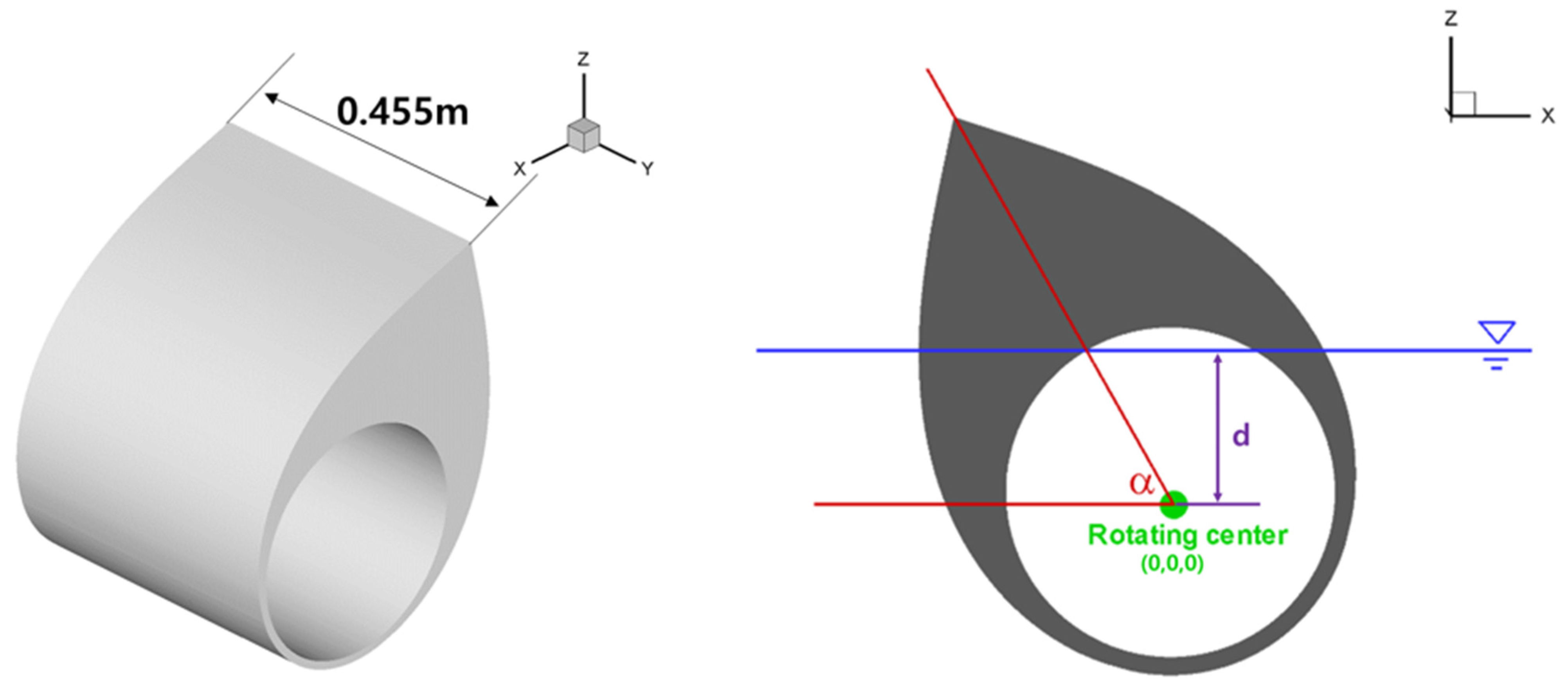
A series of CFD simulations were conducted to investigate wave-induced non-linear motion with respect to wave heights. Figure 1 shows the shape of an asymmetric rotor model with a scale ratio of 1/11, which was used for the experimental study in [22]. In addition, the origin of the body-fixed coordinate system is the rotating center, and y = 0 is half the width. The prototype of the model was optimized with a target wave height of 2.0 m and wave period of 5.1 s, which was the wave condition for Jeju, a western sea of South Korea. The principal dimensions of the rotor model are summarized in Table 1. The beak angle and draft of the rotor model are 60° and 0.17 m, respectively. In addition, the vertical distance between the free surface and the rotating center of the rotor model is 1.6 m. The rotor model has a hole at the center of the rotating axis to reduce manufacturing costs. In this study, the rotor model is assumed to be installed on a fixed large platform; hence, the other directional motions excluding the pitch motion are fixed. To understand the non-linear pitch motion characteristics, PTO damping was not considered in this study. Each of the CFD simulation results, which are calculated for the model scale, are expressed in full-scale for this study.
2.2. Wave Conditions
The CFD simulations were performed for regular wave conditions. Table 2 summarizes the CFD simulation conditions for regular waves. The wave periods were determined by considering the wave condition of Jeju in South Korea, as mentioned earlier. Five different wave heights were considered to investigate the linear and non-linear motions. In this study, the wave heights were divided into two levels: low wave heights (0.11 m, H/d = 0.06; 0.33 m, H/d = 0.18) and high wave heights (0.55 m, H/d = 0.29; 1.10 m, H/d = 0.59; 2.00 m, H/d = 1.07). In the case of low wave height conditions, for validating the CFD results, they were directly compared with the experimental results in [22].
3. Numerical Method
3.1. Numerical Schemes
STAR-CCM+ 11.06 V, which is a well-known commercial CFD software, was used in this study. In the CFD simulation, the governing equation for the incompressible flow is the continuity equation and Navier–Stokes equations, as shown in Equations (1) and (2), where is a finite volume limited to a closed surface , is fluid velocity vector including the velocity of , and is a unit vector, which is vertical to and toward the outer direction. is viscous stress tensor and is a unit vector. In addition, is gravity, is the momentum source, is time, is pressure, and is fluid density.
In this study, the 5th order Stokes wave theory was employed to generate regular waves, and the wave forcing method in STAR-CCM+ was employed to minimize wave reflections at the outlet boundary. The wave force method, which is similar to the Euler overlay method, is a blending technique. To prevent the reflection wave, an additional source term is applied to each conservation equation. Equation (3) is the new source term, where is the reference value, which is from the theoretical wave. Navier–Stokes equations discretized at a distance were employed from other theoretical solutions. Equation (3) is the newly defined source term; the source term reduces the difference between the CFD solution and undisturbed wave solution.
The forcing coefficient is given by Equation (4), where is the forcing coefficient, which is equal to in Equation (3). refers to the maximum value of and the forcing. To dampen the difference between forced and recent solutions at each simulation time, the wave forcing method, which applies the characteristics of the spatial distribution of , enables gradual application of the constraint. In addition, represents the strength of forcing and has a cosine function, as shown in Equation (4). The theoretical value of the transport equation becomes equal to the calculated value of the transport equation at each computation time when is a maximum value.
The free-surface capturing method is the Volume of Fluid (VOF). The motion equations of the rotor using the results of velocity and pressure were solved using Equations (5) and (6), where and are the total force and total moment, respectively, and and are the external force and external moment by gravity, respectively. In addition, and are the buoyancy/force/moment by pressure or viscosity. From Equations (5) and (6), the velocity and pitch angle of the rotor can be calculated.
Table 3 summarizes the numerical schemes used in this study. The convection and temporal schemes are second-order upwind and second-order, respectively. An adjustable time step was applied to maintain the target CFL number. In addition, a laminar model was determined in this study. However, the turbulent model can be very important for estimating a slamming load.
3.2. Grid System and Boundary Condition
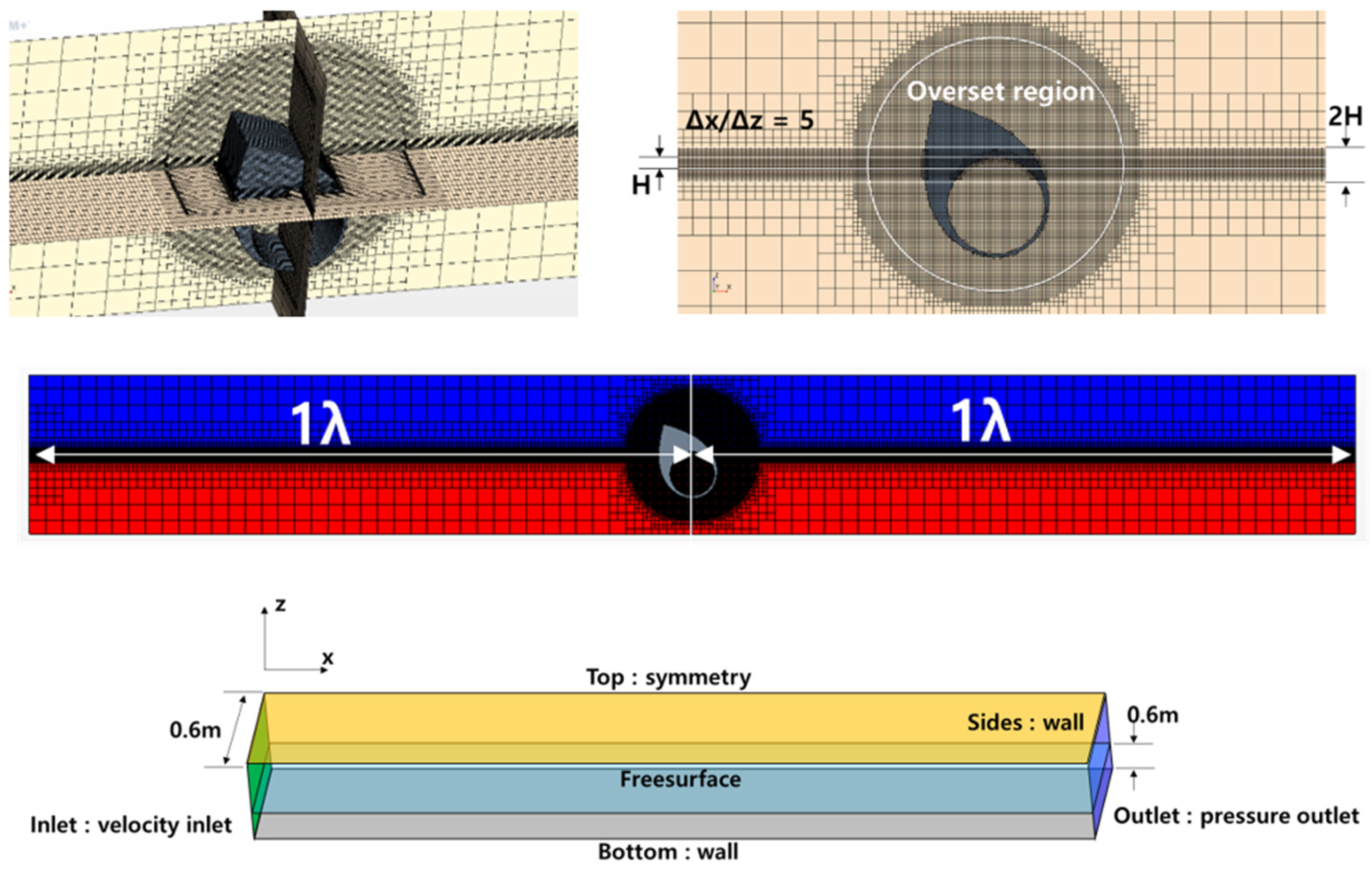
In the present CFD simulations, the breadth and wave depth of the numerical domain are set to be of the same size as the 2D wave tank at the Jeju National University, as seen in [18].
To decrease the number of grids, the forcing method was applied in the CFD simulations. Therefore, the domain length was determined to be equal to the wavelength. In this study, the grid size was determined using [23]. The upper figures in Figure 2 show the grid systems. Two refinement zones in the fluid domain and one refinement zone in the overset region were adopted around the wave region and model region. The heights of the refinement zones for the wave region were set as one time and two times the wave amplitude. The refinement zone size in the overset region was set to be equal to the one-time refinement zone size of the wave amplitude. To accurately generate the regular wave, a grid aspect ratio of 5 was applied in the wave region. In the CFDs, the prism layer for the viscous sub-layer is excluded because the viscosity of the fluid is less important in the body motion problem. The boundary conditions were as follows: the velocity inlet boundary condition was applied to the inlet part, pressure outlet boundary condition for the outlet part, and symmetry condition for the top part, and wall boundary conditions were applied to the sides, bottom, and rotor model surfaces. In addition, the total number of grids was 0.57 million.
4. Results and Discussion
4.1. Wave-Only Simulation
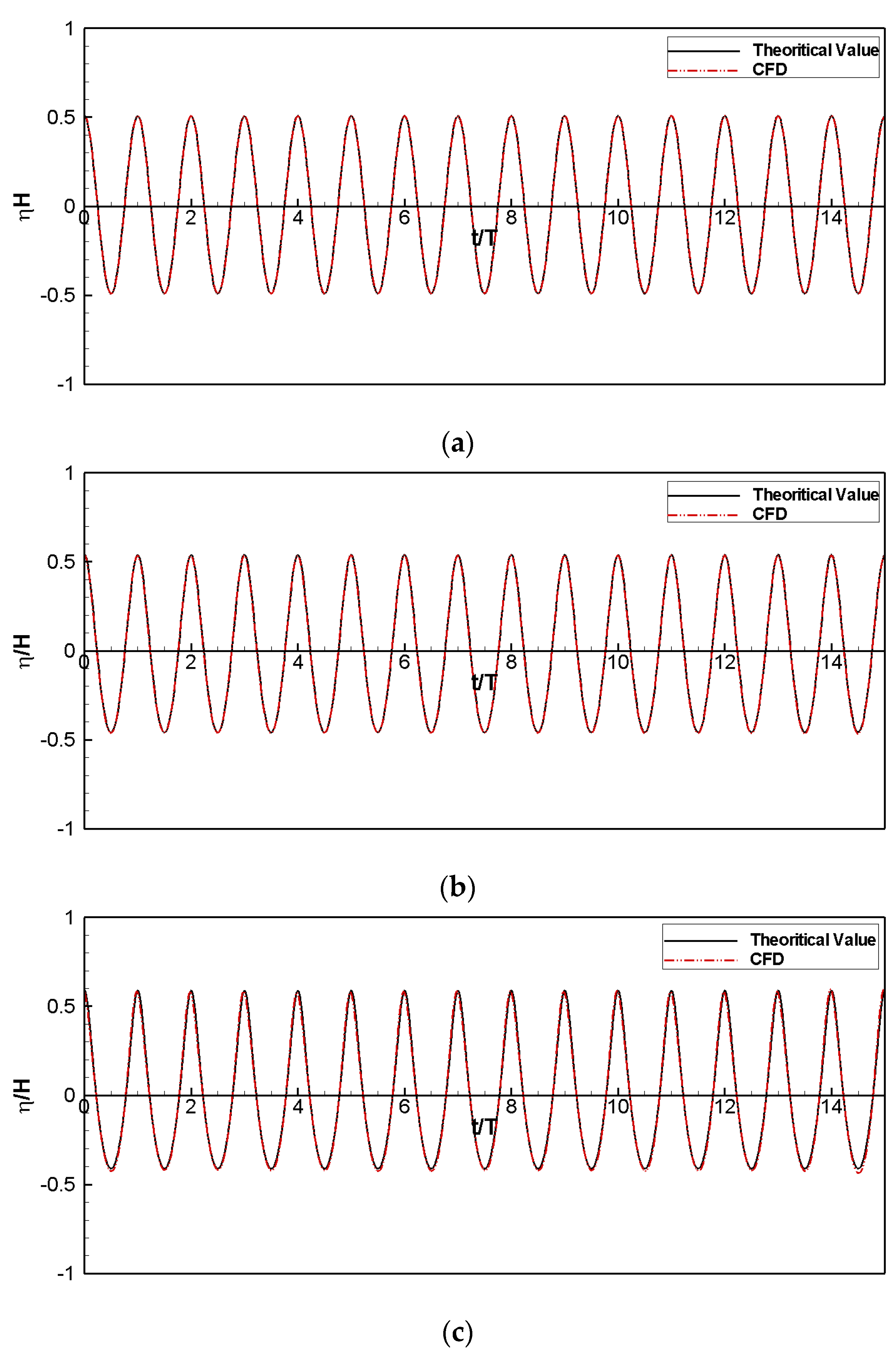
In this study, wave-only simulations were performed under three different wave conditions. In the CFD simulation, a wave period of 4.75 s was fixed, and the wave steepness was representatively determined to be 1/100, 1/50, and 1/10. The grid system is the same as in Figure 3, and the overset regions, which include the rotor, are not included in the grid system. The CFD simulation results were directly compared with the theoretical values, and the data were normalized to the input wave conditions. As shown in Figure 3, the CFD results are in good agreement with the theoretical values, and the maximum error for three different wave heights is under 1%; thus, motion simulations for the rotor were performed.
4.2. Lower Wave Heights (with Validation Results)
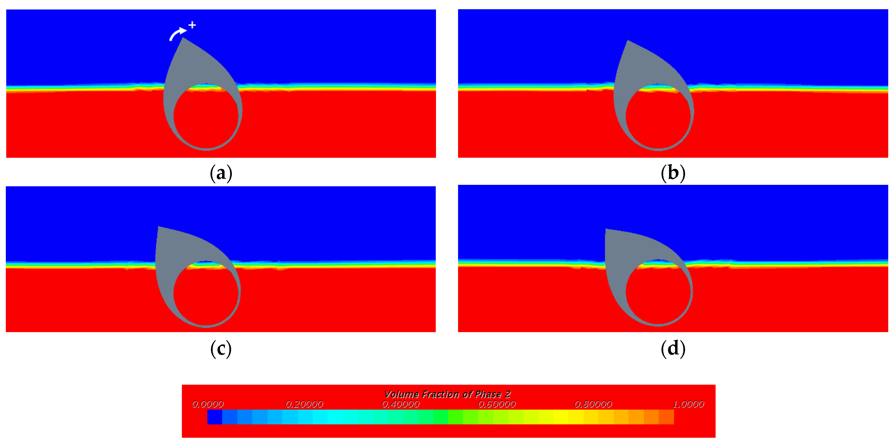
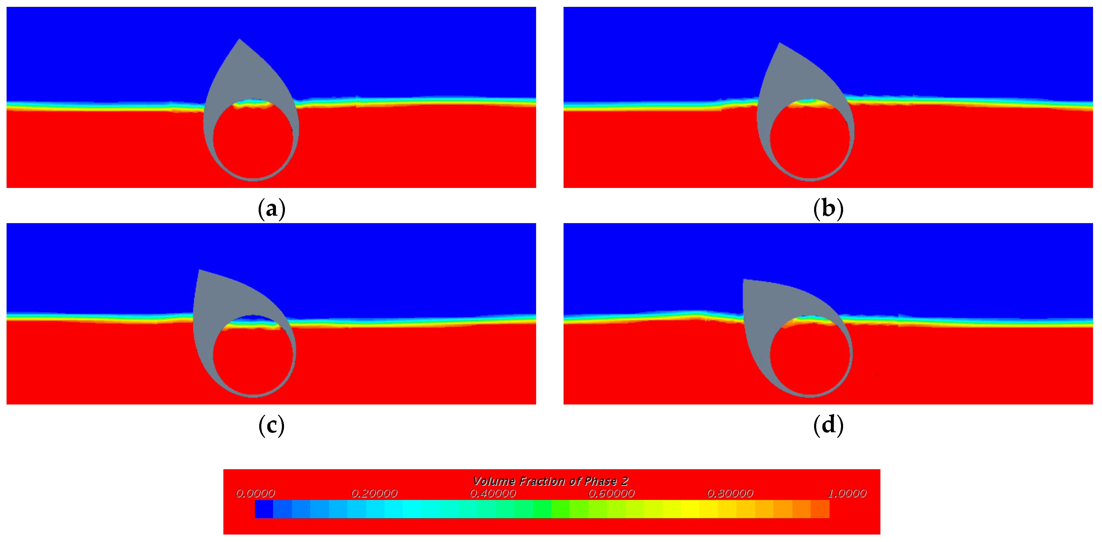
In this study, CFD simulations were performed for relatively small regular waves. For validation, the CFD results under low wave height conditions (0.11 m and 0.33 m) were directly compared with the experimental results in [22]. Figure 4 shows the snapshots for consecutive stages of the CFD results at T = 5.10 s and H = 0.11 m. In Figure 4, the positive amplitude of the rotor pitch motion is defined as rotating backward. In this study, the snapshots of the CFD simulation results were normalized to each wave period because of the repetition of pitch motion of the rotor in regular waves. In addition, 0/3 π is when the maximum positive amplitude of the rotor occurs. Figure 4 shows the slightly upward and downward movement of the rotor.
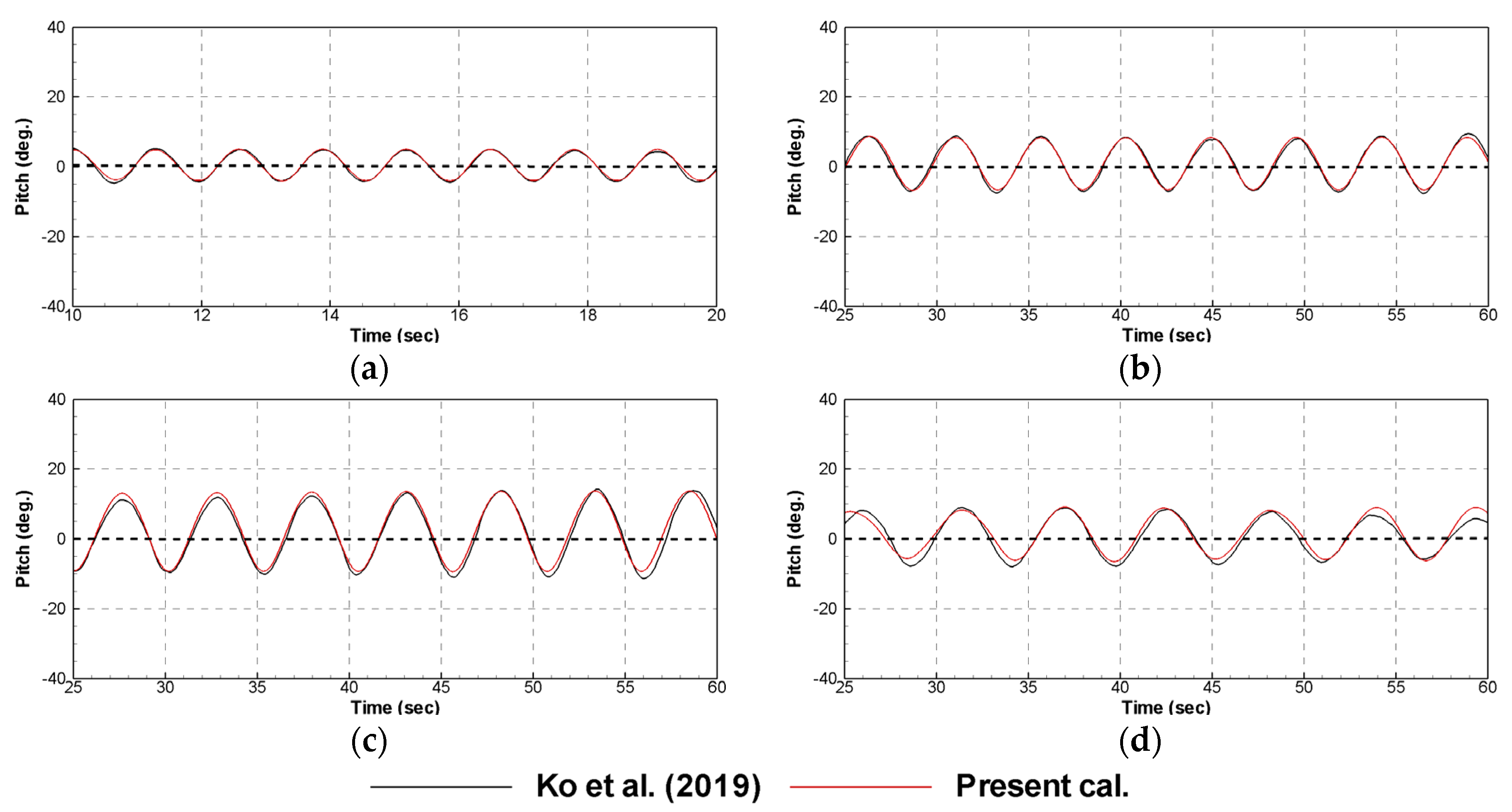
Figure 5 directly compares the time histories of pitch motions between the experimental and CFD simulation results in representative wave periods. The CFD results are in good agreement with the experimental results in [22]. In addition, it can be seen that the positive and negative amplitudes of the pitch motions are similar to each other, and the results appear to be linear motion.
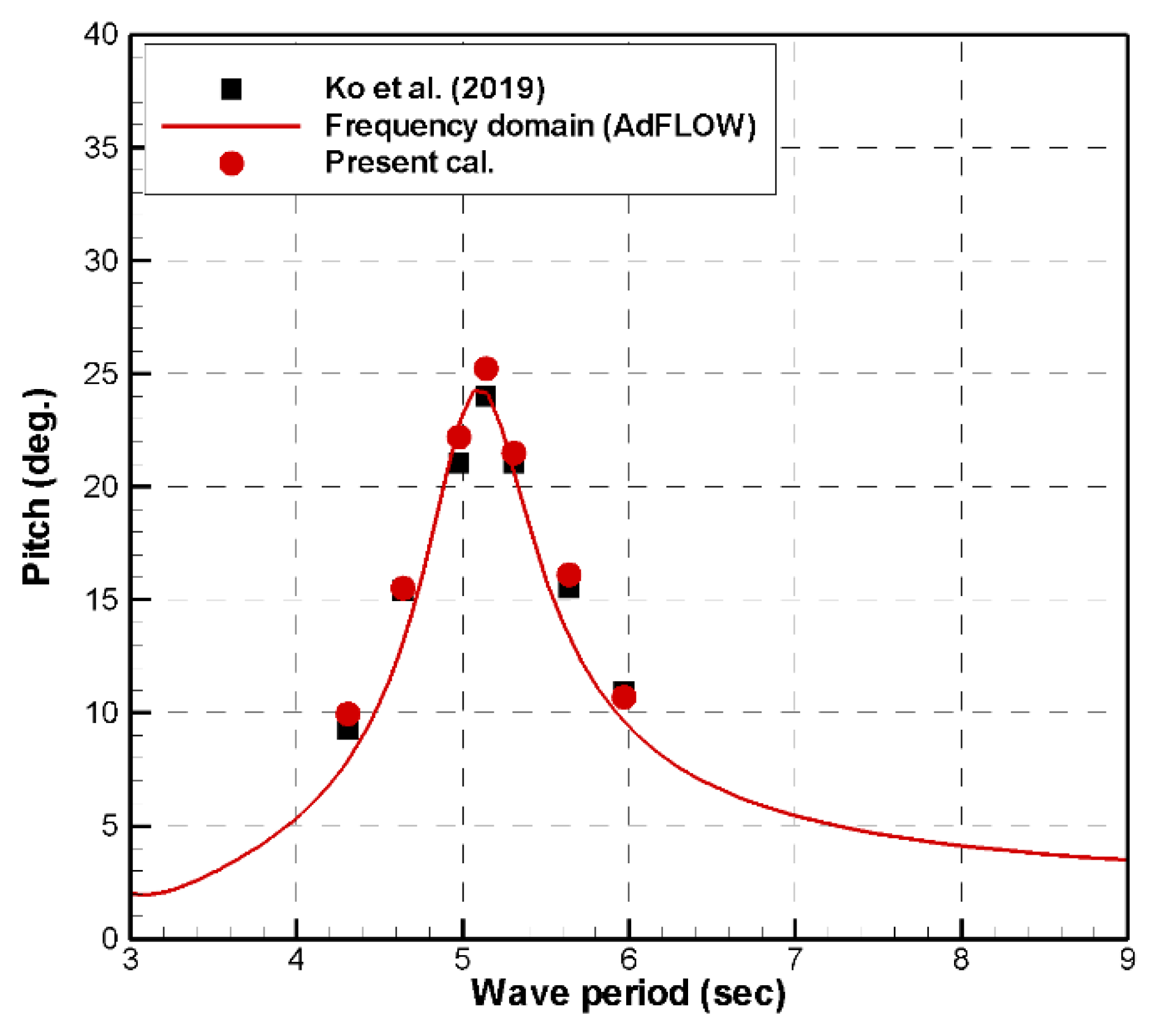
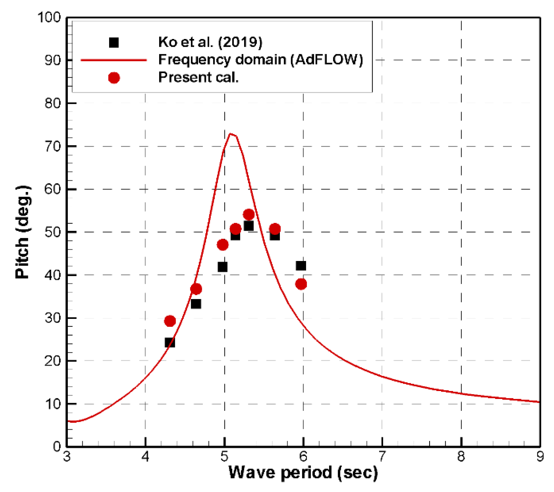
The magnitudes of the pitch motions with respect to the wave periods from the CFD simulations were directly compared with the experimental results in [22]. In addition, they were compared with the results of the frequency domain analysis (AdFLOW), which was developed as a potential-based program in the Korea Research Institute of Ships and Ocean Engineering (KRISO), where the magnitude of the pitch motion is defined as the height of the pitch motion of the rotor in Figure 5. As shown in Figure 6, the magnitudes of the pitch motions from all three methods are in good agreement, with each other because the maximum error among the three methods according to the wave periods is about 3%. In the case of a relatively lower wave height (H = 0.11 m), the incoming waves are near the linear waves, and the pitch motions further show a linear response. However, a slight non-linear response appears to have occurred near 5.10 s. Therefore, the frequency domain analysis can be useful to estimate the pitch motions of the rotor at a relatively lower wave height. As shown in Figure 6, it can be observed that the pitch resonance period of the rotor is near 5.10 s.
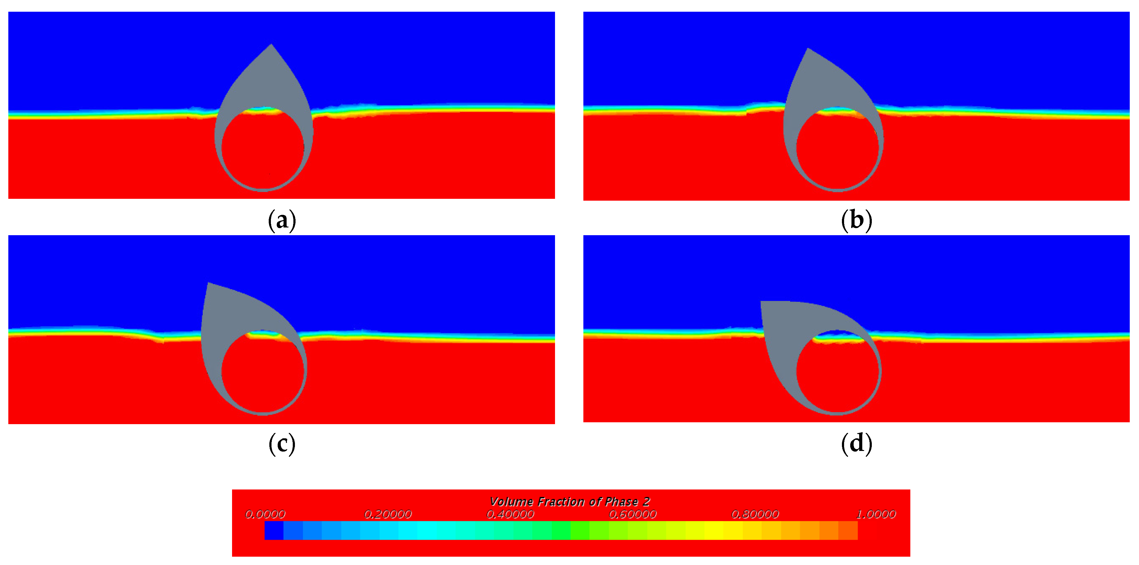
To compare the pitch motion patterns in different wave periods, Figure 7 and Figure 8 show representative snapshots from the CFD results for the wave height of 0.33 m in wave periods of 4.25 s and 5.30 s, respectively. As shown in Figure 7 and Figure 8, a relatively smaller pitch motion of the rotor occurs in a wave period of 4.25 s, while the pitch motion of the rotor relatively increases in a wave period of 5.30 s, particularly as the positive amplitude of the rotor pitch motion increases.
Figure 9 shows the comparison of time histories of the pitch motions between the experimental and CFD results for each wave period, and both these results are similar to each other. In the case of T = 4.25 s, the maximum amplitudes of the pitch motions in the positive and negative directions are similar, but the maximum positive amplitudes of the pitch motions are relatively larger than the maximum negative amplitudes of the pitch motions in the case of other wave periods. Therefore, in the case of a wave height of 0.33 m, it can be seen that the linear pitch motions and non-linear pitch motions occur.
The pitch magnitudes from the CFD simulations were directly compared with those of the experimental and frequency domain analysis results, as shown in Figure 10. The maximum error between the CFD simulation and experimental results according to the wave periods is about 5%. The frequency domain simulation result is different from the experimental and CFD results, excluding the pitch motions in relatively short-wave periods (4.25 s and 4.60 s). In the case of the pitch motions in relatively short-wave periods, the pitch motions show linear responses, as shown in Figure 9a. At this wave height, it can be seen that maximum pitch motion occurs in a wave period of 5.30 s. This is because the secondary moment of the water plane might have changed owing to the asymmetry shape of the rotor. In the case of the frequency domain simulation, the change in the secondary moment of the water plane cannot be considered. In addition, the pitch magnitudes near the wave period of 5.30 s decreased as the viscous damping increased at this wave height.
4.3. High Wave Heights
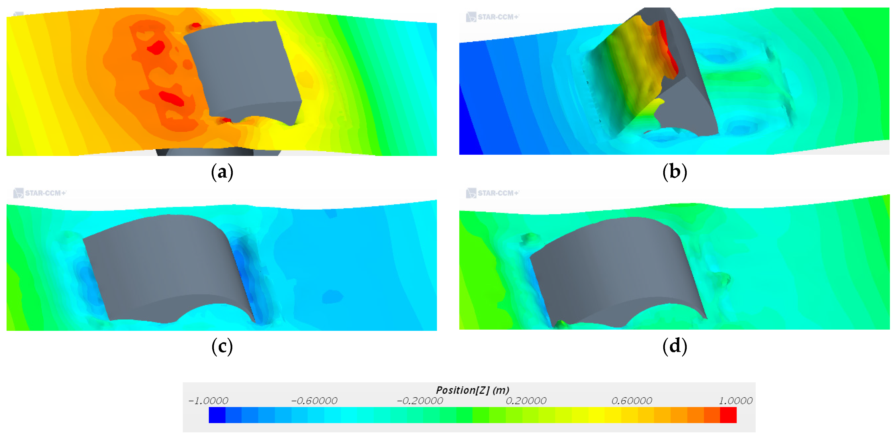
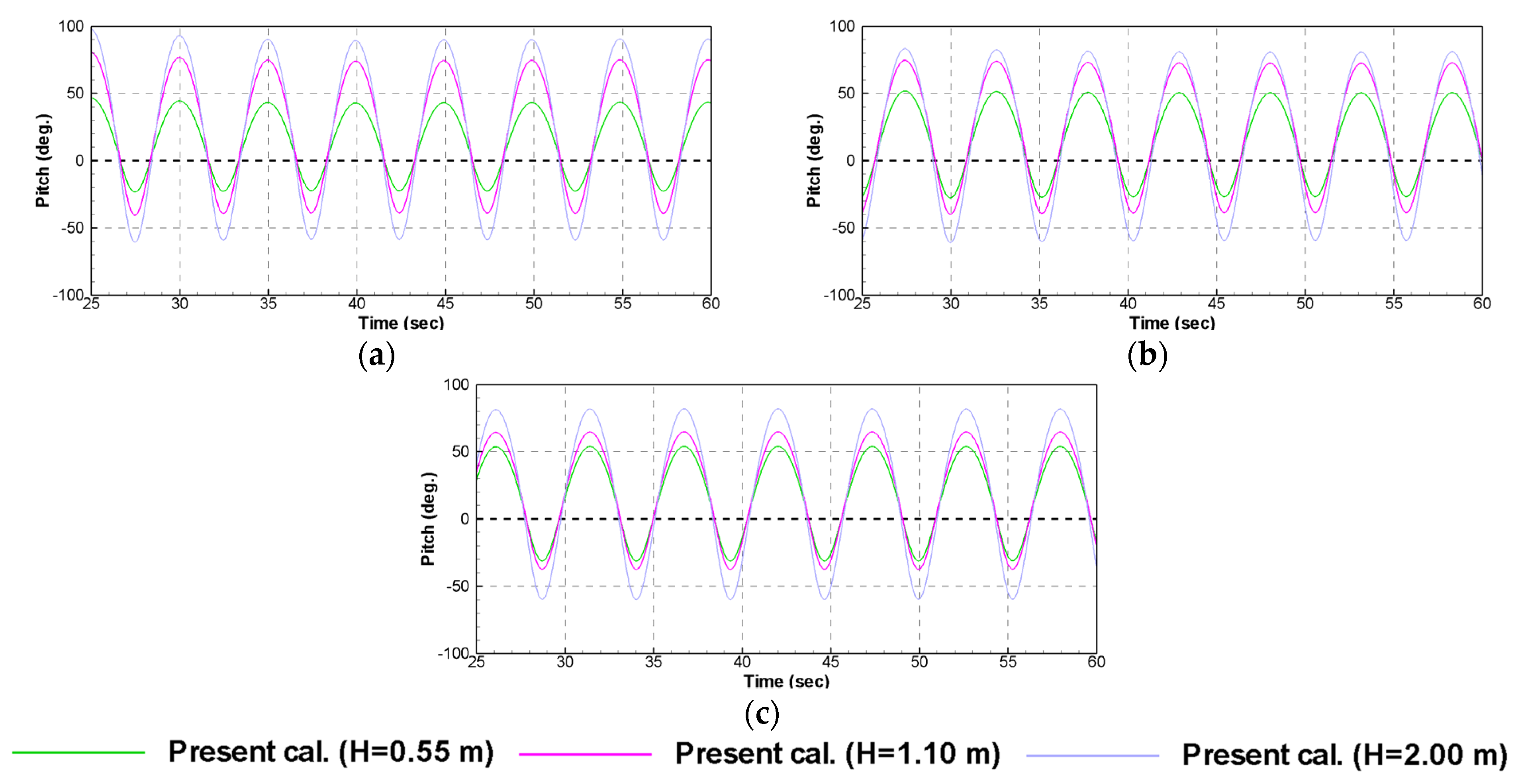
In this study, CFD simulations were performed at relatively higher wave heights. Figure 11 shows snapshots from the CFD results according to the wave heights at T = 5.10 s. The pitch motions increase with increasing wave heights, and non-linear phenomena, such as wave runup and slamming phenomena, occur on the rotor surface from a wave height of 1.10 m, as shown in Figure 11b,c and Figure 12. Figure 13 shows the representative time histories of the pitch motions of the rotor at three wave heights under representative wave periods. The differences between the positive and negative amplitudes of the pitch motions gradually increase with increasing wave height. This means that the restoring moments between the positive and negative directions can be different.
The restoring moment can be defined by Equation (7), where is the restoring moment, is the displacement volume, is the center of buoyancy in the z-direction, is the secondary moment of a water plane, is the displacement, and is the center of gravity in the z-direction. The water plane areas can change according to the pitch angles of the rotor, as shown in Figure 11. Then, the secondary moments of the water plane can change according to the pitch angles of the rotor. Finally, the restoring moments can be different according to the pitch angles of the rotor.
4.4. Characteristics of Pitch Motion
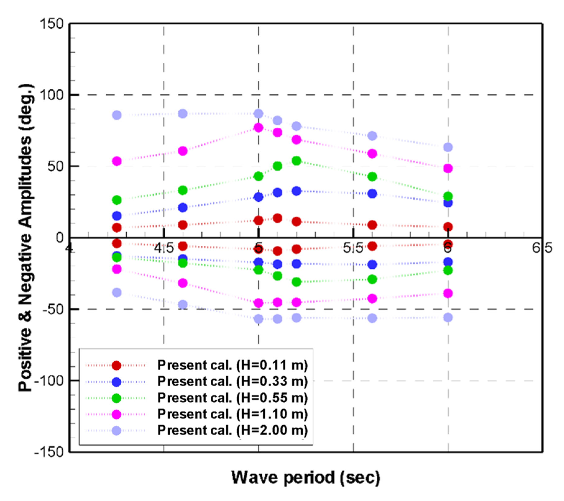
Figure 14 shows the summarized maximum amplitudes of the pitch motions in the positive and negative directions from the CFD results. The maximum amplitudes of the pitch motions in each wave condition are the average values for five periods in the pitch time histories. In the case of wave heights of 0.11 m, the differences between the maximum amplitudes of the pitch motions in the positive and negative directions appear to be relatively small in all wave periods; the maximum difference is approximately 4 deg. In addition, their differences gradually increase as the wave height increases.
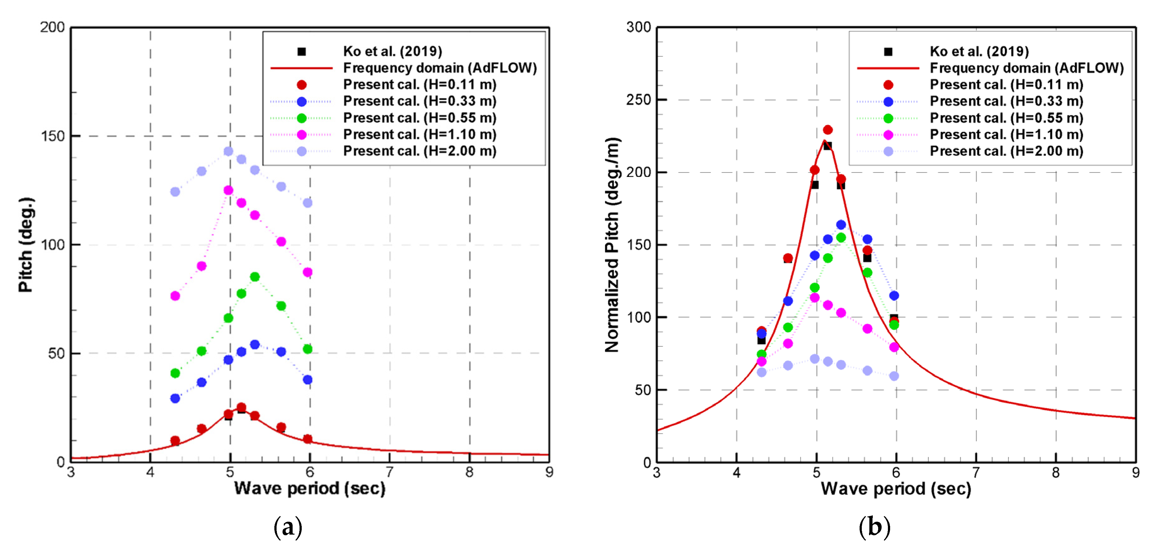
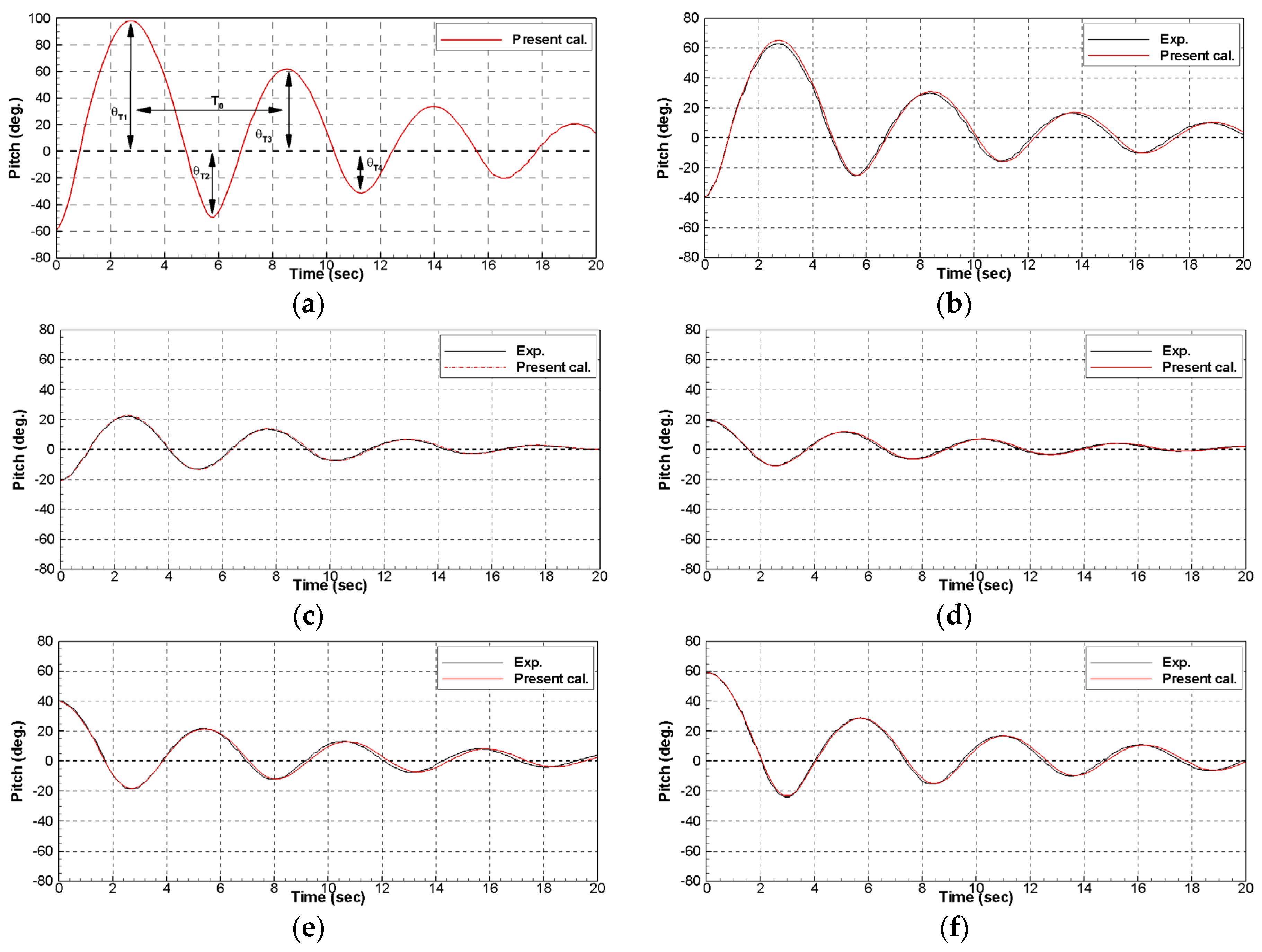
Figure 15a shows the magnitudes of the pitch motions according to the wave heights. It can be seen that the magnitudes of the pitch motions largely increase as the wave height increases. In addition, the wave periods at the maximum pitch motions at relatively higher wave heights are changed by comparing with the results for a wave height of 0.11 m. The pitch motions in Figure 15a are normalized to each wave height, as shown in Figure 15b. The magnitudes of the normalized pitch motions decrease with increasing wave heights, as shown in Figure 15b. To investigate the resonance periods and viscous damping, free-decay tests were performed from the experiments and CFD simulations in accordance with the changing initial angles of the rotor. Figure 16 shows the results from the experiments and CFD simulations. The CFD results are similar to the experimental results, and the maximum error of the pitch amplitudes in all cases is under 4% compared to the experimental results. In Figure 16a, the CFD was performed for an initial angle of −60 deg. However, the model test was not performed.
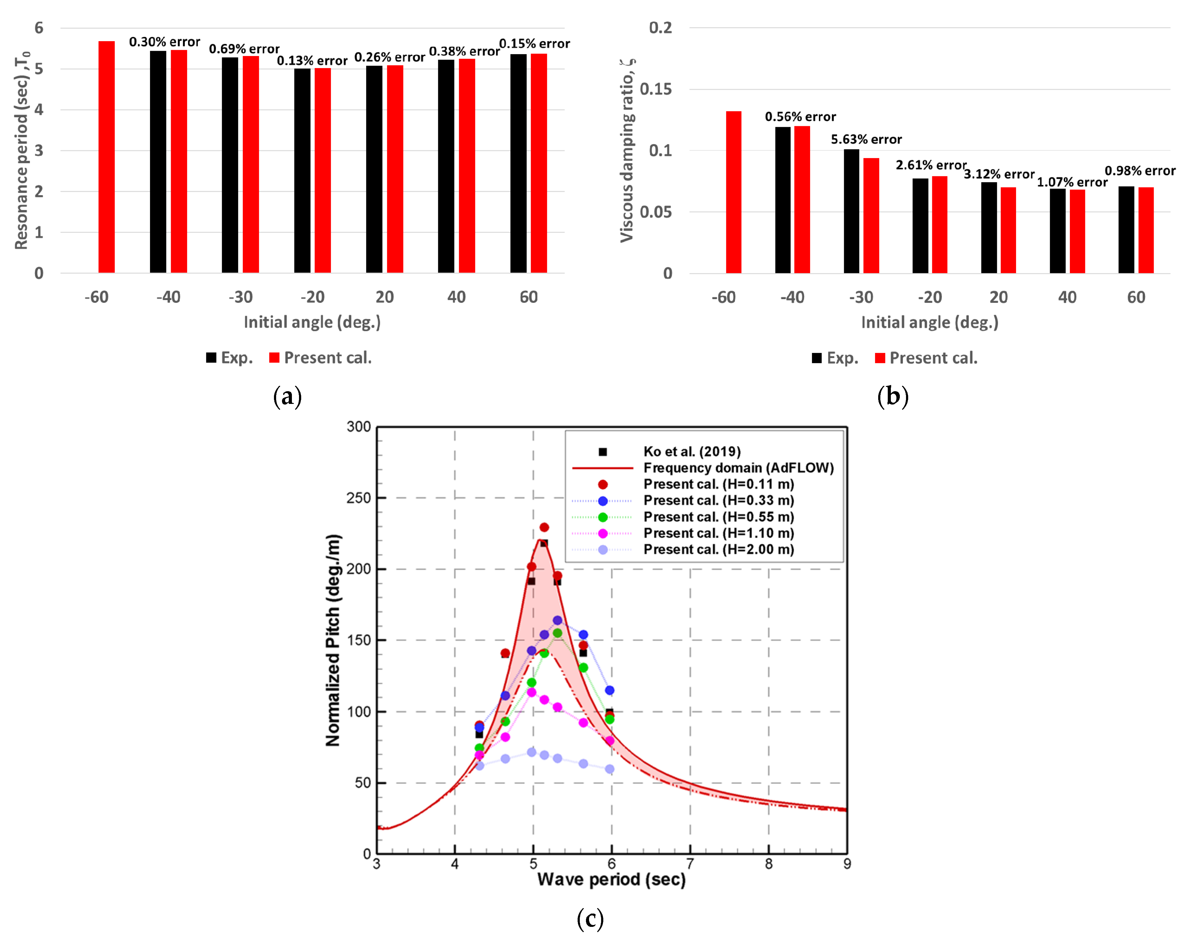
Figure 17 shows the resonance periods and viscous damping ratios from the free-decay tests by the experiments and CFD simulations including the relative errors. The resonance period and viscous damping ratio were obtained as shown in Figure 16a and Equation (8). Equation (8) refers to the study in [19]. The resonance periods slightly change depending on the initial angles of the rotor, as shown in Figure 17a. As the pitch angle of the rotor is changed, it can be found that the restoring moments also change.
As shown in Figure 17b, it can be seen that the viscous damping ratios are slightly changed in accordance with changing initial angles of the rotor. Figure 17c shows the normalized pitch motions, including the viscous damping ratio at an initial angle of −60 deg. in the frequency domain analysis. Despite applying the viscous damping ratio at −60 deg., the result is relatively larger than the CFD results for wave heights of 1.10 m and 2.00 m. In addition, it can be seen that it is difficult to consider the changing resonance wave periods with respect to the wave heights, as shown in Figure 17c.
4.5. Survey for Hydrodynamic Coefficients
To investigate the changes in the normalized pitch motions according to the wave heights, each term in the uncoupled pitch motion equation (Equation (9)) was examined. First, CFD simulations for the forced motion were conducted to investigate the added moments of inertia and radiation damping. The CFD simulations for the forced motion were performed in accordance with changes in the pitch amplitudes and oscillation periods, which were determined considering the resonance periods and magnitudes of pitch motions at a wave height of 0.55 m.
The time histories of the rotor pitch moment from the forced motion simulations can be calculated using the dynamic pressure on the rotor. To calculate the added moments of inertia and radiation damping, the time histories of the rotor pitch moments were separated into the real and imaginary parts using the Fourier series as shown in Equations (10) and (11). In addition, the added moment of inertia and radiation damping coefficients can be calculated from Equations (12) and (13).
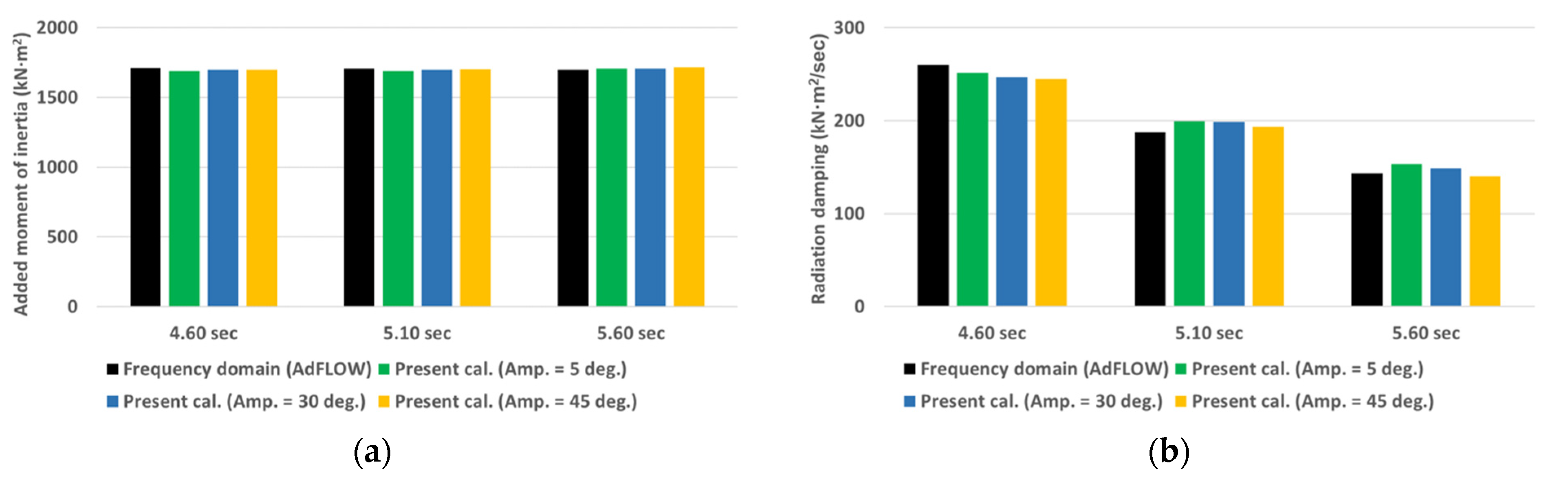
In the case of the wave heights of 1.10 m and 2.00 m, it was difficult to apply the pitch motion equation owing to the slamming phenomena, as shown in Figure 12b,c. Figure 18 shows the added moments of inertia and radiation damping from the forced motion simulations. The results of the CFD simulation and frequency domain analysis were directly compared with each other. It can be seen that the added moments of inertia and radiation damping from the CFD simulations are similar to the frequency domain analysis results. Therefore, the inertia and damping terms of the pitch motion equation would have minimal effect on the change in the normalized pitch motions.
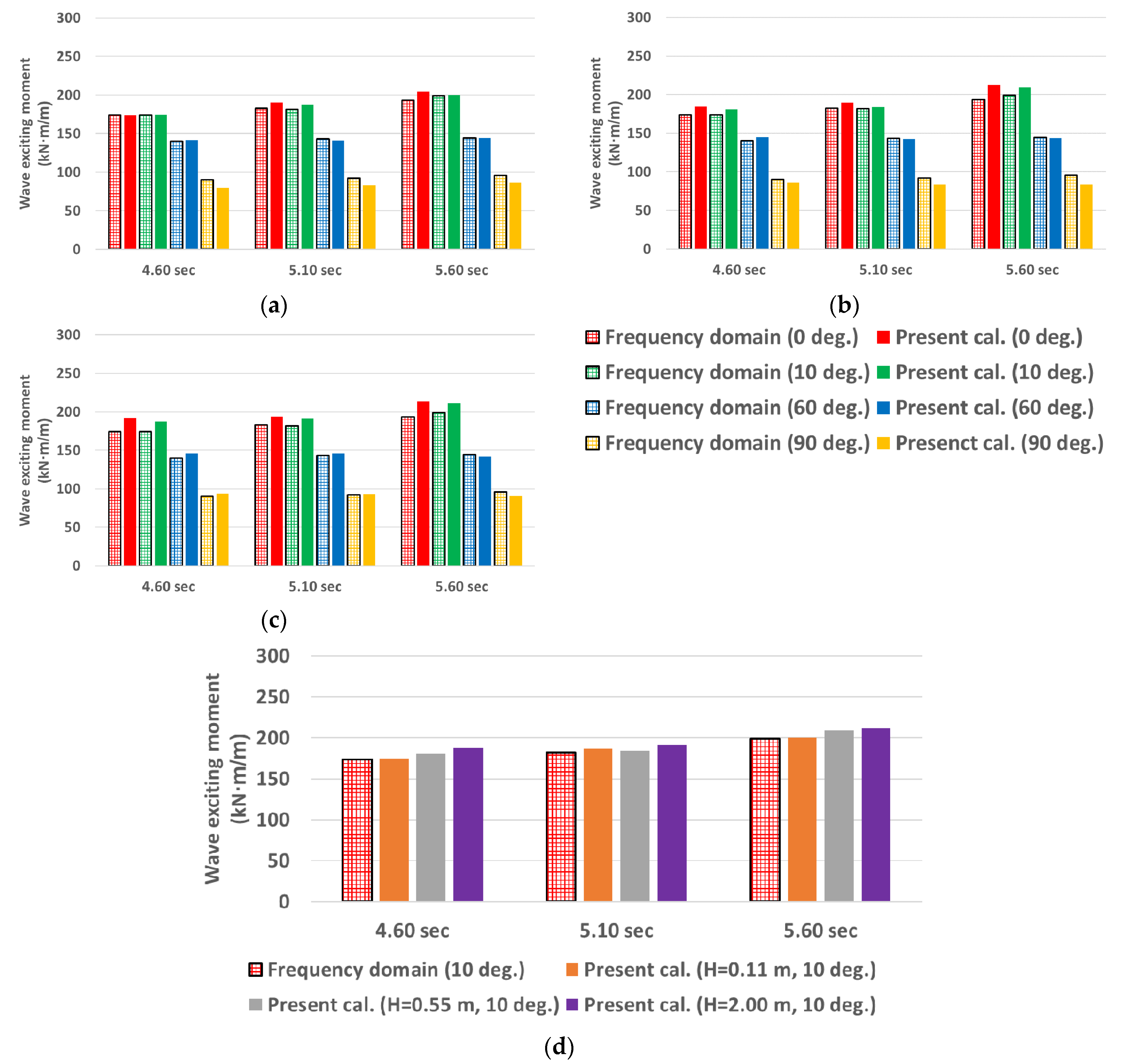
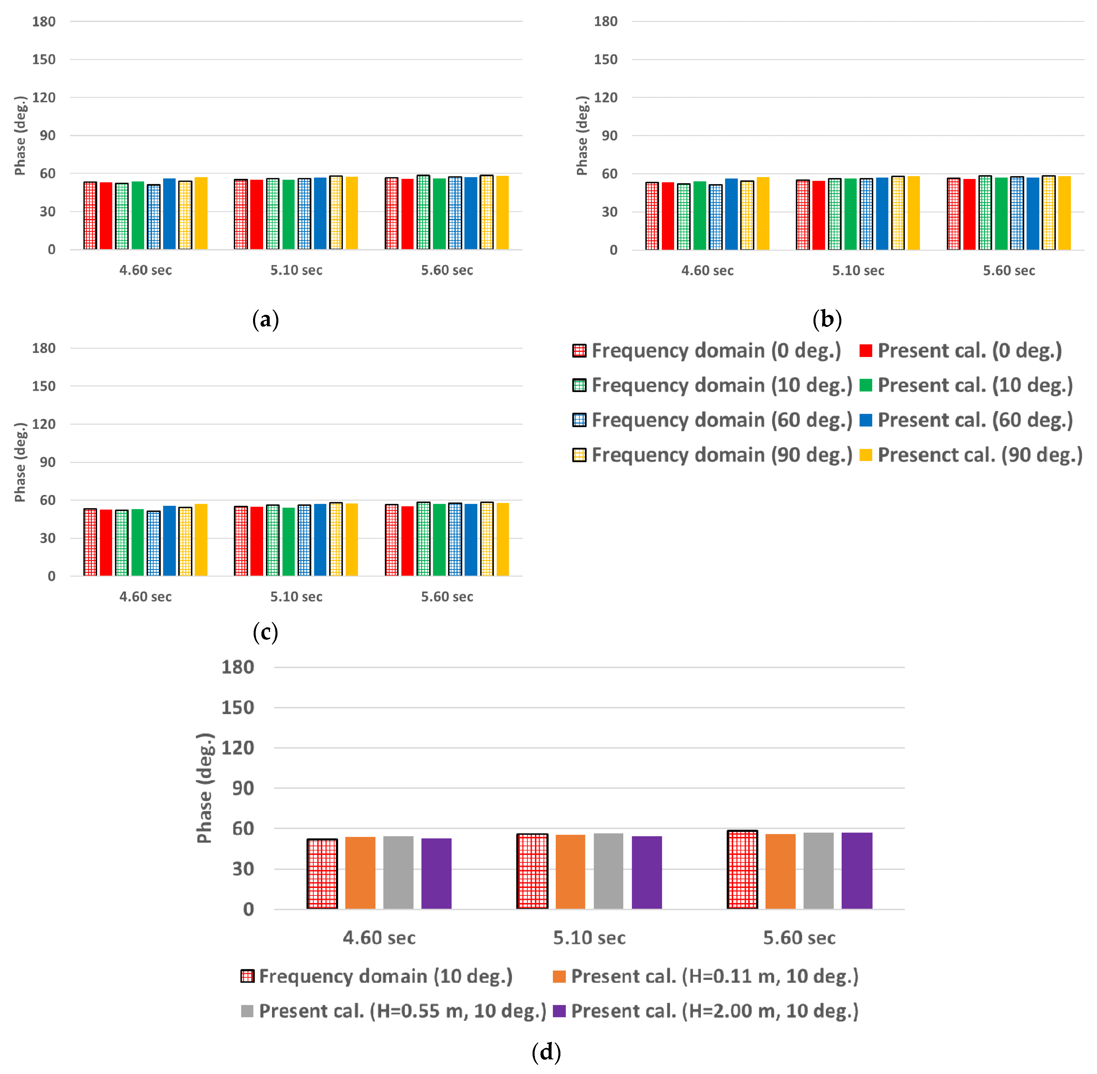
To investigate the wave exciting moments, fixed-body simulations using CFD were performed by varying the pitch angles and wave heights. Figure 19 shows the wave exciting moments from the fixed-body simulations using CFD. The CFD simulation results were directly compared with those of the frequency domain analysis. In addition, the wave exciting moments were normalized to the incident wave heights. Figure 19a–c shows the wave exciting moments at wave heights of 0.11 m, 0.55 m, and 2.00 m, respectively. It can be observed that the CFD results for three different wave heights are similar to those of the frequency domain analysis. Interestingly, the wave exciting moments at large pitch angles are changed owing to the change in the shape of the rotor, as shown by the blue and yellow bars. Figure 19d shows the wave exciting moments at a pitch angle of 10 deg. are less sensitive with respect to changes in wave heights. It can be seen that the wave exciting moments at other pitch angles show a similar trend. Figure 20 shows the phase angles, and it can be seen that the phase angles are less sensitive to changes in the wave heights and pitch angles.
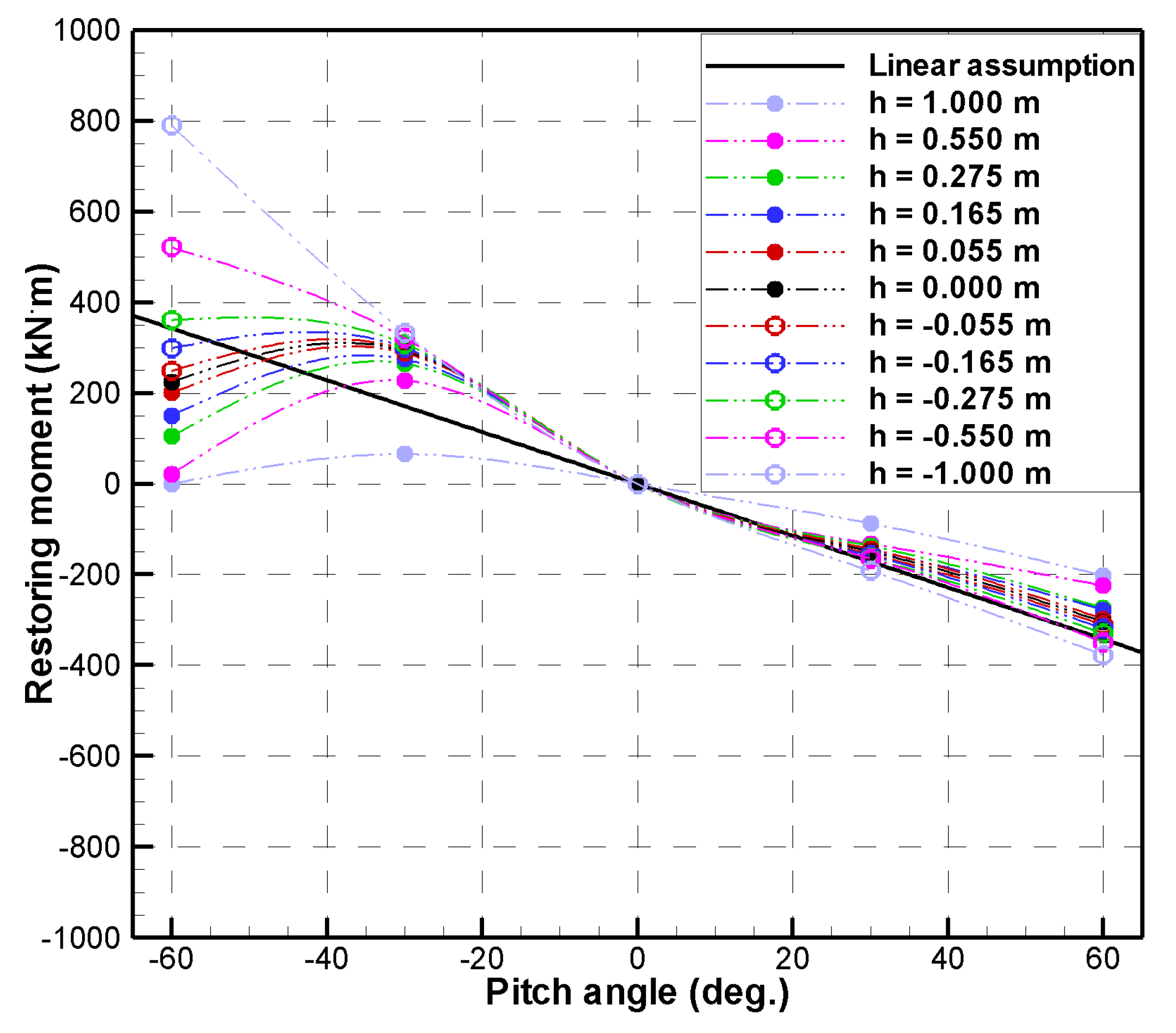
In this study, the restoring moments were investigated depending on the changes in the relative water depths (h) and pitch angles, as shown in Figure 21. The restoring moments can change with the pitch angles, and the restoring moments can also change with the relative water depths, which are caused by the wave heights of the incoming waves with a rotating rotor. However, changes in the relative water depths due to the ever-changing wave elevations and pitch angles of the rotor are difficult to consider in order to estimate the restoring moments. Therefore, the relative water depths were assumed based on the crests and troughs of the incoming waves in the static condition, and the restoring moments were estimated according to the pitch angles at each water depth. The calculated restoring moments are compared with the results from the linear assumption. In the case of the linear assumption, the restoring moments change linearly according to the pitch angles. However, owing to the changes in the secondary moment of the water plane, the restoring moments of the rotor change depending on the relative water depths and pitch angles. Therefore, the variations of the restoring moments in the motion equation should be considered to estimate the pitch motions. In [19], the author performed a time-domain analysis and modified normalized pitch motions according to wave heights ranging from 0.02 m to 0.08 m by changing the restoring moments. The experimental and time-domain simulation results were similar to each other at relatively low wave heights. In the case of higher wave height conditions, the resonance periods of the rotor and magnitudes of normalized pitch motions between the experimental and time-domain simulation results were different. Regarding the difference between the experimental and time-domain results in higher wave conditions, research in [19] noted that the differences could occur due to a slamming effect and viscous effect.
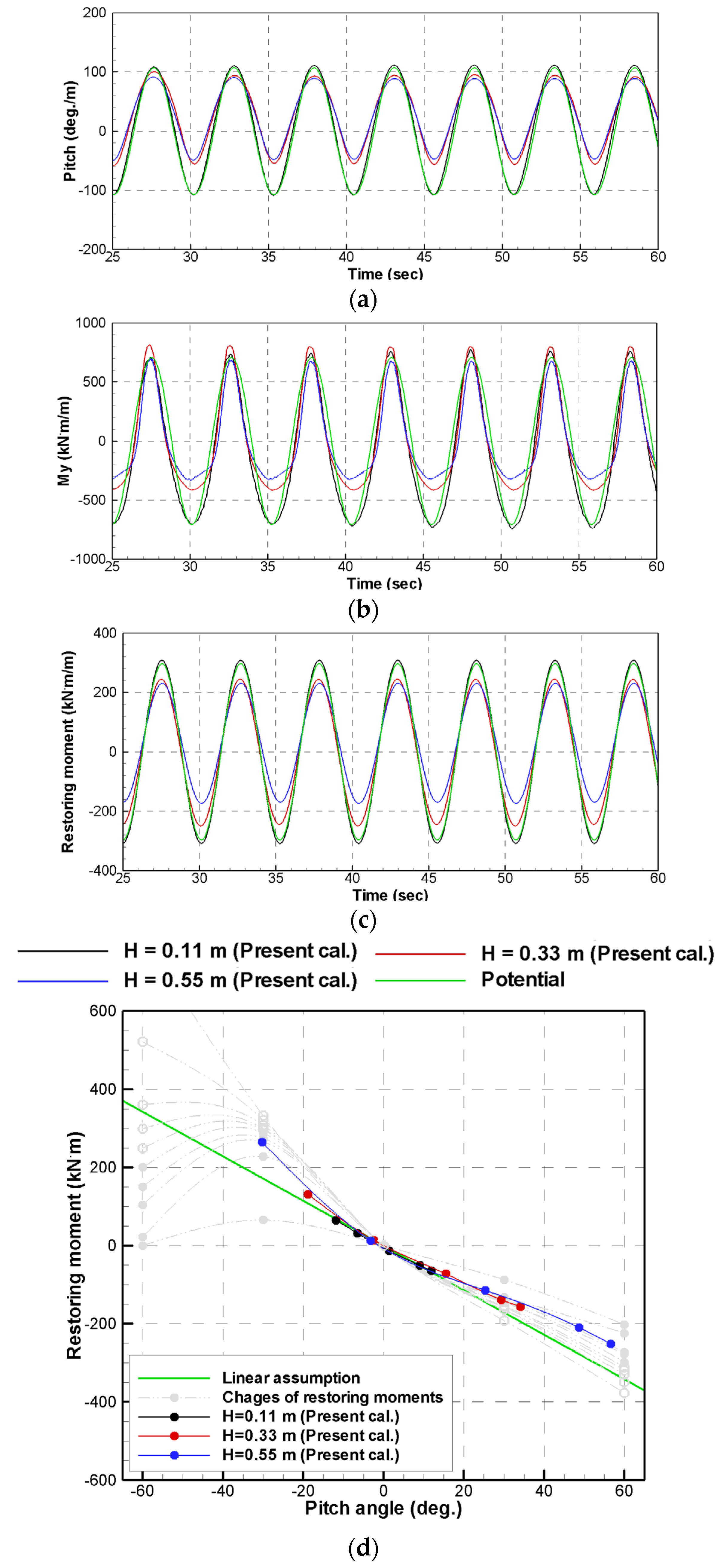
In this study, the time histories of the pitch motions, pitch moments, and restoring moments at T = 5.1 s, H = 0.11 m, 0.33 m, and 0.55 m were directly compared with the results based on linear potential theory, as shown in Figure 22, and the results were normalized to the wave heights. The time histories of the pitch motion, pitch moment, and restoring moment for the linear potential theory were estimated from the motion equation using the hydrodynamic coefficients of the frequency domain analysis, and the results were named as ‘potential’.
In the case of the CFD results, the pitch motions and pitch moments were directly calculated from the CFD simulations, and the time histories of the restoring moments for different wave heights were directly estimated from the hydrodynamic coefficients and viscous damping using the CFD simulations. Equation (14) is the pitch motion equation for estimating the restoring moment. As shown in Figure 22a, the time histories of the pitch motions from the CFD simulations at a wave height of 0.11 m are similar to the potential result. The pitch motions from the CFD simulations at relatively high wave heights are relatively smaller than the potential result, notably the negative amplitudes. The trends of the pitch moments are also similar to the trends of the pitch motions, as shown in Figure 22b. As shown in Figure 22c, the restoring moments at wave heights of 0.33 m and 0.55 m are relatively smaller than the CFD simulation and potential results in a wave height of 0.11 m. This is because the restoring moment cannot be linear in the case of the rotor, as shown in Figure 21. The restoring moments from the CFD simulations were directly compared for close examinations, as shown in Figure 22d. In the case of a wave height of 0.11 m, the restoring moment is linear, but the restoring moments in relatively high wave heights are non-linear. As a result, the magnitudes of the normalized pitch motions can decrease with increasing wave heights because of the changing restoring moments. From this study, the changes in the restoring moments and wave exciting moments at large pitch angles should be considered when applying the linear potential theory, and a time-domain analysis can be used for this purpose.
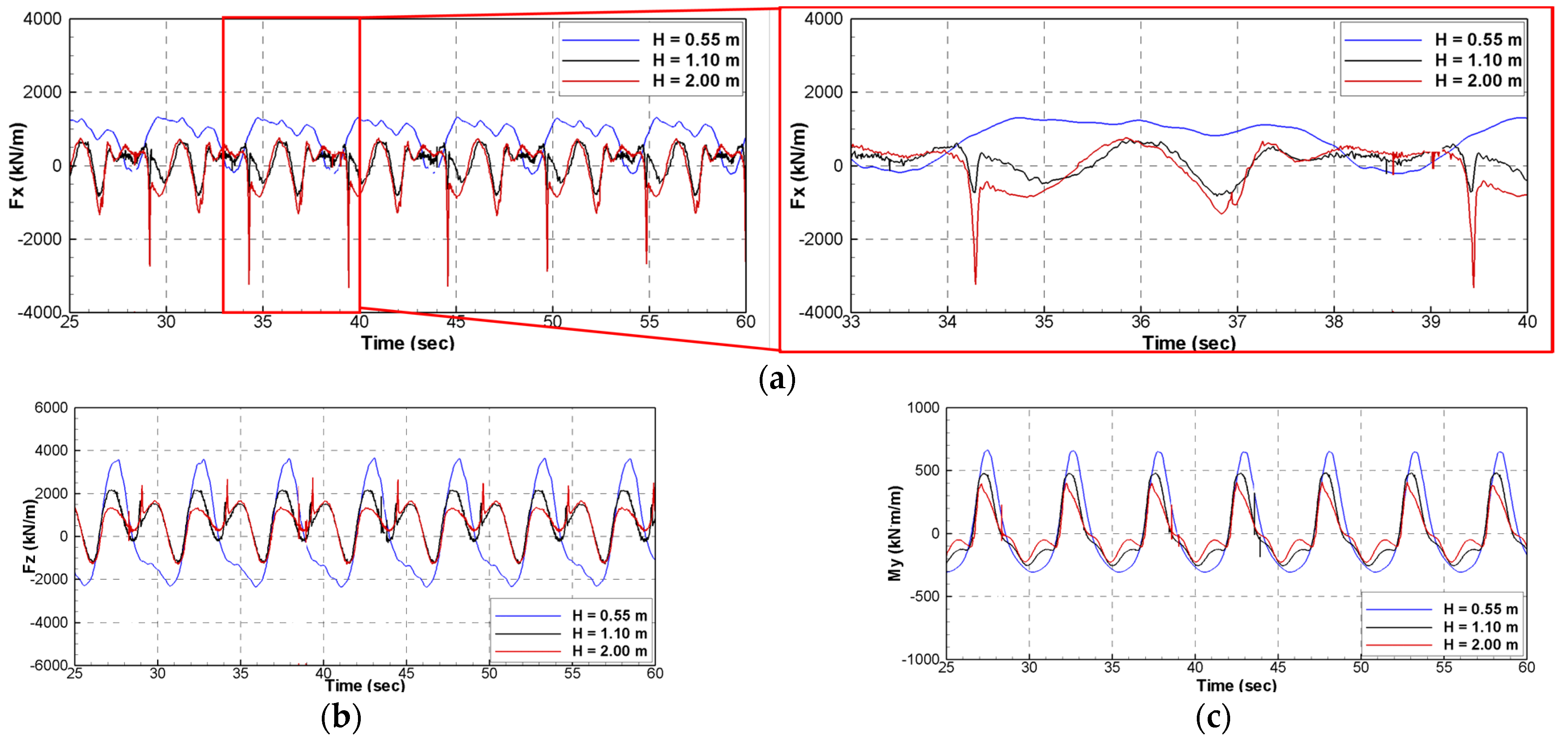
Figure 23 shows the representative time histories for each of the directional forces at T = 5.1 s and H = 0.55 m, 1.10 m, and 2.00 m. The forces were normalized to the wave heights. In the case of higher wave heights, it can be seen that the slamming impact forces occur by large pitch motions, as shown in Figure 23a,b. In the case of the horizontal force, it can be seen that the slamming impact force during a short time occurs approximately three times the static force, as shown in Figure 23a. Owing to the slamming impact forces, the time histories of the pitch moments in Figure 23c have non-sinusoidal shapes. The pitch motion of the rotor can be affected by the change in the restoring moment and non-linear phenomena. From the results, the non-linear phenomena probably lead to additional damping, as shown in Figure 17c, and the resonance period can be shifted to a relatively shorter period owing to the increase in the water mass by the wave runup. A high wave height can occur in a real sea; therefore, a non-linear motion analysis including the viscous, such as the CFD method, can be required in the designing phase of a rotor. From this study, it can be found that the variation of the pitch motions at relatively high wave heights can occur owing to the changing restoring moments and non-linear phenomena (e.g., wave runup and slamming).
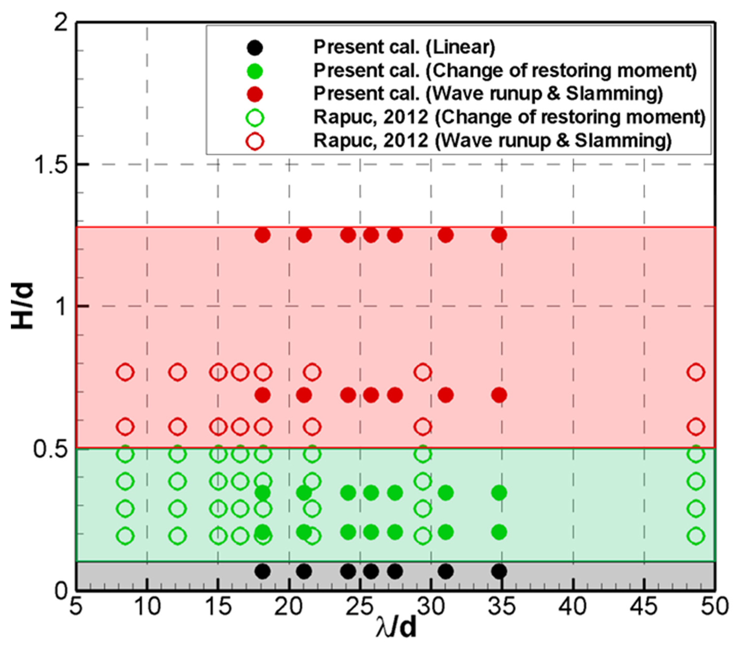
In this study, the pitch motion characteristics were classified according to the physical phenomena, as shown in Figure 24. To propose more useful information, the results were complemented using the study results in [19]. In Figure 24, the filled circles are the present study results and the empty circles are the study results in [19]. In the case of the black circles, the rotor pitch motion can be estimated using the linear potential theory, such as frequency domain analysis, and the region of H/d might be under 0.1. In the case of a green circle, the change in the restoring moment should be considered to estimate the rotor pitch motion, and the region of H/d might range from 0.1 to 0.5. In addition, the change in the wave exciting moment at a large pitch angle can be considered. For this purpose, both a time-domain analysis and direct simulation using CFD could be used, but the frequency domain analysis can be difficult. Finally, the CFD simulation should be used to estimate the pitch motion of the rotor because the slamming phenomena can occur in H/d of more than 0.5. In the study in [19], the non-linear motion and slamming phenomenon occurred at similar boundaries. However, categorizing H/d from this study might not be accurate. If several studies on the Salter’s duck-type rotor are performed, the region of H/d and that of λ/d can be more accurately classified. In addition, this study was performed under the pitch-only free condition of the rotor, wave-only condition, and deep water condition. Therefore, it is necessary to consider a freely floating condition, wave with tidal condition, shallow water condition, etc. Generally, a large absorbed power can be generated in the large motion of a WEC. To design a Salter’s duck-type rotor capable of generating a large absorbed power, the representative wave condition is first determined in a target sea. Then, the performance of the rotor is investigated using a relatively fast frequency domain analysis. In addition, the regions for H/d and λ/d are investigated in Figure 24, and the performances of the rotor are re-checked using an appropriate design tool. Finally, the designed rotor suitable to the target sea can be suggested, and the absorbed power can be investigated using the proper design tool with PTO damping.
5. Conclusions
A CFD study was conducted to investigate the pitch motion characteristics of a WEC rotor. From a series of numerical simulations, the following conclusions were drawn.
- In this study, the normalized pitch results from the frequency domain analysis in H = 0.11 m and H = 0.33 m have maximum error of about 3% compared to the experimental results. The maximum error for the normalized pitch results between the CFD simulations and experiments is about 5%. In the free-decay test, the maximum error of the resonance period between the CFD simulations and experiments is under 1%, and the maximum error of viscous damping ratio is under 6%. Therefore, the CFD simulation results can be used to interpret the non-linear behavior of the rotor.
- For a wave height of 0.11 m, the CFD simulation results are in good agreement with the experimental and frequency domain analysis results. As shown in the time histories of the pitch motions, the positive and negative amplitudes of the pitch motions from the CFD simulations have symmetrical shapes, which appear to be linear motions. Therefore, the obtained linear solution is sufficient in the case of a low wave height, and the resonance period of the rotor is located near 5.1 s.
- Considering the pitch motion equation, the added moments of inertia, radiation damping, and wave exciting moments for relatively small pitch angles do not change considerably. However, the wave excitation moments can be changed at relatively large pitch angles. Furthermore, at relatively higher wave heights, the magnitudes of the normalized pitch motions and resonance periods are changed by changing the restoring moments. In addition, the pitch motions are affected by non-linear phenomena, such as wave runup and slamming, and it is difficult to estimate the pitch motions of the rotor using the linear potential theory.
- According to the physical phenomena, the regions are classified into three types. In the case of H/d under 0.1, the linear potential theory, such as a frequency domain analysis, can be directly applied to estimate the pitch motions of the rotor. In H/d ranging from 0.1 to 0.5, a time-domain analysis could be used to estimate the pitch motions of the rotor by considering the changes in the restoring moments and wave exciting moments at large pitch angles. In addition, the time-domain analysis and a direct simulation using CFD could be used to estimate the pitch motions of the rotor. In the case of H/d over 0.5, where wave runup and slamming phenomena occur, CFD simulations should be used to estimate the pitch motions of the rotor.
- In this study, a selection method for an appropriate design tool was suggested to design a Salter’s duck-type rotor suitable for a sea. This method has several constraints; hence, it can be useful in the initial design phase for a Salter’s duck-type rotor. Therefore, the regions of H/d and λ/d, including a model condition, a tidal, a PTO damping, etc., will be modified. In the future, a guideline for a WEC design will be suggested, including stochastic results from irregular wave tests.
Author Contributions
Formal analysis, Y.-J.H. and J.-Y.P.; writing—original draft preparation, Y.-J.H. and J.-Y.P.; writing—review and editing, S.-H.S.; supervision and project administration, S.-H.S. and J.-Y.P. All authors have read and agreed to the published version of the manuscript.
Funding
This research received no external funding.
Institutional Review Board Statement
Not applicable.
Informed Consent Statement
Not applicable.
Data Availability Statement
Data available in a publicly accessible repository.
Acknowledgments
This study was funded by “Development of WECAN for the Establishment of Integrated Performance and Structural Safety Analytical Tools of Wave Energy Converter” (PES3980).
Conflicts of Interest
The authors declare no conflict of interest.
References
- Cho, C.H.; Lee, Y.H.; Kim, H.J.; Choi, Y.D.; Kim, B.S. Ocean Energy Engineering; Dasom: Siheung-si, Korea, 2006; pp. 154–169. [Google Scholar]
- Evans, D.V. A theory for wave-power absorption by oscillating bodies. J. Fluid. Mech. 1976, 77, 1–25. [Google Scholar] [CrossRef]
- Yeung, R.W. Added mass and damping of a vertical cylinder in finite-depth waters. Appl. Ocean Res. 1981, 3, 119–133. [Google Scholar] [CrossRef]
- Evans, D.V.; Mciver, P. Added mass and damping of a sphere section in heave. Appl. Ocean Res. 1984, 6, 45–53. [Google Scholar] [CrossRef]
- Evans, D.V. Maximum wave-power absorption under motion constraints. Appl. Ocean Res. 1981, 3, 200–203. [Google Scholar] [CrossRef]
- Budal, K.; Falnes, J. Wave power conversion by point absorbers: A Norwegian project. Int. J. Ambient Energy 1982, 3, 59–67. [Google Scholar] [CrossRef]
- Cummins, W.E. The impulse response function and ship motions. Schiffstechnik 1962, 47, 101–109. [Google Scholar]
- Falcão, A.F.O. Modelling and control of oscillating-body wave energy converters with hydraulic power take-off and gas accumulator. Ocean Eng. 2007, 34, 2021–2032. [Google Scholar] [CrossRef]
- Zurkinden, A.S.; Ferri, F.; Beatty, S.; Kofoed, J.P.; Kramer, M.M. Non-linear numerical modeling and experimental testing of a point absorber wave energy converter. Ocean Eng. 2014, 78, 11–21. [Google Scholar] [CrossRef]
- Do, H.T.; Dinh, Q.T.; Nguyen, M.T.; Phan, C.B.; Dang, T.D.; Lee, S.; Park, H.G.; Ahn, K.K. Effects of non-vertical linear motions of a hemispherical-float wave energy converter. Ocean Eng. 2015, 109, 430–438. [Google Scholar] [CrossRef]
- Gao, H.; Liang, R. Performance analysis of axisymmetric floating energy harvesters and influences of parameters and shape variation. Int. J. Energy Res. 2018, 43, 2057–2074. [Google Scholar] [CrossRef]
- Ransley, E.J. RANS-VOF Modelling of the Wavestar Point Absorber. Renewable Energy 2017, 49–65. [Google Scholar] [CrossRef] [Green Version]
- Windt, C.; Faedo, N.; García-Violini, D.; Peña-Sanchez, Y.; Davidson, J.; Ferri, F.; Ringwood, J.V. Validation of a CFD-based numerical wave tank model of the 1/20th scale wavestar wave energy converter. Fluids 2020, 5, 112. [Google Scholar] [CrossRef]
- Brito, M.; Canelas, R.B.; García-Feal, O.; Domínguez, J.M.; Crespo, A.J.C.; Ferreira, R.M.L.; Neves, M.G.; Teixeira, L. A numerical tool for modelling oscillating wave surge converter with nonlinear mechanical constraints. Renew. Energy 2020, 146, 2024–2043. [Google Scholar] [CrossRef]
- Brito, M.; Ferreira, R.M.L.; Teixeira, L.; Neves, M.G.; Canelas, R.B. Experimental investigation on the power capture of an oscillating wave surge converter in unidirectional waves. Renew. Energy 2020, 151, 975–992. [Google Scholar] [CrossRef]
- Salter, S.H. Wave power. Nature 1974, 249, 720–724. [Google Scholar] [CrossRef]
- Mynett, A.E.; Serman, D.D.; Mei, C.C. Characteristics of salter’s cam for extracting energy from ocean waves. Appl. Ocean Res. 1979, 1, 13–20. [Google Scholar] [CrossRef]
- Poguluri, S.K.; Bae, Y.H. A Study on performance assessment of WEC Rotor in the Jeju western waters. Ocean Syst. Eng. 2018, 8, 361–380. [Google Scholar]
- Rapuc, S. Numerical Study of the WEPTOS Single Rotor. Master’s Thesis, Aalborg University, Aalborg, Denmark, 2012. [Google Scholar]
- Pecher, A.; Kofoed, J.P.; Marchalot, T. Experimental Study on a Rotor for WEPTOS; DCE Contract Report No. 110; Aalborg University: Aalborg, Denmark, 2011. [Google Scholar]
- Pecher, A.; Kofoed, J.P.; Larsen, T.; Marchalot, T. Experimental study of the WEPTOS wave energy converter. In Proceedings of the 31st International Conference on Ocean, Offshore and Arctic Engineering, Rio de Janeiro, Brazil, 1–6 July 2012. [Google Scholar]
- Ko, H.S.; Kim, D.E.; Cho, I.H.; Bae, Y.H. Numerical and experimental study for nonlinear dynamic behavior of an asymmetric wave energy converter. In Proceedings of the 29th International Ocean and Polar Engineering Conference, Honolulu, HI, USA, 16–21 June 2019; International Society of Offshore and Polar Engineering: Mountain View, CA, USA, 2019. [Google Scholar]
- Hwang, S.C.; Nam, B.W.; Ha, Y.J.; Kim, K.H.; Hong, S.Y.; Cho, S.K. Numerical Analysis on Sidewall Green Water Problem of a Ship-shaped FPSO in Bow Quartering Sea. In Proceedings of the 29th International Ocean and Polar Engineering Conference, Honolulu, HI, USA, 16–21 June 2019. [Google Scholar]
Figure 1.
The shape of the rotor model for the numerical simulation.

Figure 2.
Grid system for the numerical simulations.

Figure 3.
Wave simulation results: (a) λ/H = 1/100; (b) λ/H = 1/150; (c) λ/H = 1/10.

Figure 4.
Snapshots of the side view for the numerical simulation (T = 5.10 s, H = 0.11 m): (a) Phase = 0/3 π; (b) phase = 1/3 π; (c) phase = 2/3 π; (d) phase = 3/3 π.
Figure 4.
Snapshots of the side view for the numerical simulation (T = 5.10 s, H = 0.11 m): (a) Phase = 0/3 π; (b) phase = 1/3 π; (c) phase = 2/3 π; (d) phase = 3/3 π.

Figure 5.
Comparison for the time histories of the pitch motions between the experimental and numerical simulation results (H = 0.11m): (a) T = 4.25 s; (b) T = 4.60 s; (c) T = 5.10 s; (d) T = 5.60 s.
Figure 5.
Comparison for the time histories of the pitch motions between the experimental and numerical simulation results (H = 0.11m): (a) T = 4.25 s; (b) T = 4.60 s; (c) T = 5.10 s; (d) T = 5.60 s.

Figure 6.
Comparison of the magnitude of the pitch motions according to the wave periods (H = 0.11 m).
Figure 6.
Comparison of the magnitude of the pitch motions according to the wave periods (H = 0.11 m).

Figure 7.
Snapshots of the side view for the numerical simulation (T = 4.25 s, H = 0.33 m): (a) Phase = 0/3 π; (b) phase = 1/3 π; (c) phase = 2/3 π; (d) phase = 3/3 π.
Figure 7.
Snapshots of the side view for the numerical simulation (T = 4.25 s, H = 0.33 m): (a) Phase = 0/3 π; (b) phase = 1/3 π; (c) phase = 2/3 π; (d) phase = 3/3 π.

Figure 8.
Snapshots of the side view for the numerical simulation (T = 5.30 s, H = 0.33 m): (a) Phase = 0/3 π; (b) phase = 1/3 π; (c) phase = 2/3 π; (d) phase = 3/3 π.
Figure 8.
Snapshots of the side view for the numerical simulation (T = 5.30 s, H = 0.33 m): (a) Phase = 0/3 π; (b) phase = 1/3 π; (c) phase = 2/3 π; (d) phase = 3/3 π.

Figure 9.
Comparison for the time histories of the pitch motions between the experimental and numerical simulation results (H = 0.33 m): (a) T = 4.25 s; (b) T = 5.00 s; (c) T = 5.30 s; (d) T = 6.00 s.
Figure 9.
Comparison for the time histories of the pitch motions between the experimental and numerical simulation results (H = 0.33 m): (a) T = 4.25 s; (b) T = 5.00 s; (c) T = 5.30 s; (d) T = 6.00 s.

Figure 10.
Comparison of the magnitude of the pitch motions according to the wave periods (H = 0.33 m).
Figure 10.
Comparison of the magnitude of the pitch motions according to the wave periods (H = 0.33 m).

Figure 11.
Snapshots of the side view for the numerical simulation (T = 5.10 s): (a) Phase = 0/3 π; (b) phase = 1/3 π; (c) phase = 2/3 π; (d) phase = 3/3 π.
Figure 11.
Snapshots of the side view for the numerical simulation (T = 5.10 s): (a) Phase = 0/3 π; (b) phase = 1/3 π; (c) phase = 2/3 π; (d) phase = 3/3 π.

Figure 12.
Snapshots of the perspective view from the numerical simulation (T = 5.10 s, H = 2.00 m): (a) Phase = 0/3 π; (b) phase = 1/3 π; (c) phase = 2/3 π; (d) phase = 3/3 π.
Figure 12.
Snapshots of the perspective view from the numerical simulation (T = 5.10 s, H = 2.00 m): (a) Phase = 0/3 π; (b) phase = 1/3 π; (c) phase = 2/3 π; (d) phase = 3/3 π.

Figure 13.
Comparison of the time histories of pitch motions in several wave heights and wave periods: (a) T = 5.00 s; (b) T = 5.10 s; (c) T = 5.30 s.
Figure 13.
Comparison of the time histories of pitch motions in several wave heights and wave periods: (a) T = 5.00 s; (b) T = 5.10 s; (c) T = 5.30 s.

Figure 14.
Summarized results of the pitch motions for the positive and negative amplitudes.

Figure 15.
Comparison of the magnitudes of pitch motions and normalized pitch motions: (a) Pitch motion; (b) normalized pitch motion.
Figure 15.
Comparison of the magnitudes of pitch motions and normalized pitch motions: (a) Pitch motion; (b) normalized pitch motion.

Figure 16.
Comparison of the time histories between the experimental and numerical results for free-decay tests: (a) Initial angle = −60 deg.; (b) initial angle = −40 deg.; (c) initial angle = −20 deg.; (d) initial angle = 20 deg.; (e) initial angle = 40 deg.; (f) initial angle = 60 deg.
Figure 16.
Comparison of the time histories between the experimental and numerical results for free-decay tests: (a) Initial angle = −60 deg.; (b) initial angle = −40 deg.; (c) initial angle = −20 deg.; (d) initial angle = 20 deg.; (e) initial angle = 40 deg.; (f) initial angle = 60 deg.

Figure 17.
Comparison of the resonance period, and the viscous damping ratios between the experimental and numerical results for free-decay tests: (a) Resonance period; (b) viscous damping ratio; (c) normalized pitch motion when applying the largest viscous damping.
Figure 17.
Comparison of the resonance period, and the viscous damping ratios between the experimental and numerical results for free-decay tests: (a) Resonance period; (b) viscous damping ratio; (c) normalized pitch motion when applying the largest viscous damping.

Figure 18.
Comparison of the added moments of inertia and radiation damping by the forced motion simulations: (a) Added moments of inertia; (b) radiation damping.
Figure 18.
Comparison of the added moments of inertia and radiation damping by the forced motion simulations: (a) Added moments of inertia; (b) radiation damping.

Figure 19.
Comparison of the wave exciting moments by the fixed body simulations: (a) H = 0.11 m; (b) H = 0.55 m; (c) H = 2.00 m; (d) wave exciting moments at a pitch angle of 10 deg.
Figure 19.
Comparison of the wave exciting moments by the fixed body simulations: (a) H = 0.11 m; (b) H = 0.55 m; (c) H = 2.00 m; (d) wave exciting moments at a pitch angle of 10 deg.

Figure 20.
Comparison of the phase angles by the fixed body simulations: (a) H = 0.11 m; (b) H = 0.55 m; (c) H = 2.00 m; (d) phase angles at a pitch angle of 10 deg.
Figure 20.
Comparison of the phase angles by the fixed body simulations: (a) H = 0.11 m; (b) H = 0.55 m; (c) H = 2.00 m; (d) phase angles at a pitch angle of 10 deg.

Figure 21.
Comparison of the estimated restoring moments.

Figure 22.
Comparison of the time histories for the potential and CFD results (T = 5.10 s): (a) Pitch; (b) pitch moment; (c) restoring moment; (d) change in restoring moment.
Figure 22.
Comparison of the time histories for the potential and CFD results (T = 5.10 s): (a) Pitch; (b) pitch moment; (c) restoring moment; (d) change in restoring moment.

Figure 23.
Comparisons of the time histories for each of the directional forces (T = 5.10 s): (a) Surge force; (b) heave force; (c) pitch moment.
Figure 23.
Comparisons of the time histories for each of the directional forces (T = 5.10 s): (a) Surge force; (b) heave force; (c) pitch moment.

Figure 24.
Categorization according to the physical phenomena.


Table 1.
Principal dimensions of the rotor.
| Model | Prototype | |
|---|---|---|
| Scale ratio | 1/11 | |
| Beak angle (deg.) | 60 | |
| Inner hole radius (m) | 0.182 | 2.00 |
| Draft/Depth of rotating center (m) | 0.170 | 1.87 |
| Width (m) | 0.455 | 5.00 |
| Vertical distance between free-surface and rotating center (m) | 1.600 | 17.60 |
| CGX (m) | −0.0930 | −1.02 |
| CGZ (m) | 0.0998 | 1.10 |
| Mass (kg) | 13.6505 | 18,169 |
| IYY (kg m2) | 0.4934 | 7223.87 |
Table 2.
Wave conditions.
| Wave Period, T (s) | Wave Length (m) | kh | kH |
|---|---|---|---|
| 4.25 | 28.20 | 1.47 | 0.025 |
| 0.074 | |||
| 0.123 | |||
| 0.245 | |||
| 0.446 | |||
| 4.60 | 33.04 | 1.26 | 0.021 |
| 0.063 | |||
| 0.105 | |||
| 0.209 | |||
| 0.380 | |||
| 5.00 | 39.03 | 1.06 | 0.018 |
| 0.053 | |||
| 0.089 | |||
| 0.177 | |||
| 0.322 | |||
| 5.10 | 40.61 | 1.02 | 0.017 |
| 0.051 | |||
| 0.085 | |||
| 0.170 | |||
| 0.309 | |||
| 5.30 | 43.86 | 0.95 | 0.016 |
| 0.047 | |||
| 0.079 | |||
| 0.158 | |||
| 0.287 | |||
| 5.60 | 48.96 | 0.85 | 0.014 |
| 0.042 | |||
| 0.071 | |||
| 0.141 | |||
| 0.257 | |||
| 6.00 | 56.21 | 0.74 | 0.012 |
| 0.037 | |||
| 0.061 | |||
| 0.123 | |||
| 0.224 |
Table 3.
Numerical schemes for the numerical simulations.
| Discretization Scheme | Finite Volume Method (FVM) |
|---|---|
| Pressure and velocity field | Semi-implicit method for pressure-linked equation (SIMPLE) |
| Time step | Adjustable time step (target CFL number = 0.5) |
| Sub-iterations | 10 |
| Convection schemes | Second-order upwind |
| Temporal schemes | Second-order |
| Turbulence model | (laminar) |
Publisher’s Note: MDPI stays neutral with regard to jurisdictional claims in published maps and institutional affiliations. |
© 2021 by the authors. Licensee MDPI, Basel, Switzerland. This article is an open access article distributed under the terms and conditions of the Creative Commons Attribution (CC BY) license (https://creativecommons.org/licenses/by/4.0/).
Share and Cite
MDPI and ACS Style
Ha, Y.-J.; Park, J.-Y.; Shin, S.-H. Numerical Study of Non-Linear Dynamic Behavior of an Asymmetric Rotor for Wave Energy Converter in Regular Waves. Processes 2021, 9, 1477. https://0-doi-org.brum.beds.ac.uk/10.3390/pr9081477
AMA Style
Ha Y-J, Park J-Y, Shin S-H. Numerical Study of Non-Linear Dynamic Behavior of an Asymmetric Rotor for Wave Energy Converter in Regular Waves. Processes. 2021; 9(8):1477. https://0-doi-org.brum.beds.ac.uk/10.3390/pr9081477
Chicago/Turabian StyleHa, Yoon-Jin, Ji-Yong Park, and Seung-Ho Shin. 2021. "Numerical Study of Non-Linear Dynamic Behavior of an Asymmetric Rotor for Wave Energy Converter in Regular Waves" Processes 9, no. 8: 1477. https://0-doi-org.brum.beds.ac.uk/10.3390/pr9081477
Note that from the first issue of 2016, this journal uses article numbers instead of page numbers. See further details here.