Data-Driven State Prediction and Sensor Fault Diagnosis for Multi-Agent Systems with Application to a Twin Rotational Inverted Pendulum

Abstract

When a multi-agent system is subjected to faults, it is necessary to detect and classify the faults in time. This paper is motivated to propose a data-driven state prediction and sensor fault classification technique. Firstly, neural network-based state prediction model is trained through historical input and output data of the system. Then, the trained model is implemented to the real-time system to predict the system state and output in absence of fault. By comparing the predicted healthy output and the measured output, which can be abnormal in case of sensor faults, a residual signal can be generated. When a sensor fault occurs, the residual signal exceeds the threshold, a fault classification technique is triggered to distinguish fault types. Finally, the designed data-driven state prediction and fault classification algorithms are verified through a twin rotational inverted pendulum system with leader-follower mechanism.

1. Introduction

Monitoring the condition of complex systems in real-time can save valuable time and cost to maintain the system. Fault diagnosis can detect process anomalies and classify the types of anomalies, and has hence drawn enormous attention (e.g., [1,2,3]). In survey papers [4] and [5], the methods of fault diagnosis are divided into model-based, signal-based, knowledge-based, and hybrid/active methods. Knowledge-based method is also named data-driven method, where a fault diagnosis model is built through historical data rather than precise mathematical model. Therefore, a data-driven method is suitable for complex systems that are difficult to obtain an accurate model or whose signal is unknown. Data-driven fault diagnosis has been applied to real systems such as wind turbine system [6], high-speed trains [7], and induction motor drive system [8], etc.

On the other hand, many modern engineering systems are modeled as multi-agent systems (MASs), where two or more agents are communicated through a designed protocol to work cooperatively [9,10]. Due to the communication, a fault in one agent can degrade performance of its neighbors, and even the whole network. Therefore, an effective fault diagnosis technique is crucial for MAS. Furthermore, a fault alarm from one agent can be induced by its neighboring agents, hence, fault diagnosis for multi-agent system is more challenging compared with single agent system. A variety of fault diagnosis approaches have been developed for MAS recently [11,12]. Most existing work of MAS is based on a precise state-space model of each agent as well as their communication, e.g., [13,14,15]. However, the communication between agents can be unknown. Thus, it is difficult to establish an accurate mathematical model. As a result, data-driven fault diagnosis plays an important role in complex MAS.

Among various data driven fault diagnosis methods [16,17,18,19,20], the neural network can convert fault diagnosis into a multi-label classification problem, and automatically learn the features of the original data. However, storing and leaning a large amount of data in real-time is challenging for the computation and communication device/software. In order to deal with the limited capability of the device/software, event-triggered mechanize [21,22] and distributed methods [23] have been hot topics in recent years. Specifically, event-triggered fault diagnosis methods have been developed in [21] and [22], where the mathematical model of the system is assumed to be known. Nevertheless, when model and communication of MAS are not available, the above event-triggered methodologies are not applicable. Therefore, it is motivated to develop event-triggered data driven fault diagnosis for MAS with unknown mathematical model and unknown communication.

In this paper, a residual-triggered fault diagnosis technique is proposed for MAS. Specifically, a neural network-based state prediction model is established through training historical data offline. Then, online comparison of real state/output and the predicted state/output can generate a residual signal, which indicates whether there is a fault. If the residual exceeds the threshold, it triggers a fault classification training process to identify and locate the fault. This residual-triggered fault diagnosis method does not depend on a mathematical model and communication information. Moreover, online identification of a fault is implemented only in case of fault, hence the data transmission and calculation are reduced. A real experiment on leader-follower inverted pendulum demonstrates the effectiveness of the developed algorithm. The contribution includes: 1. Residual-triggered data-driven fault diagnosis for MAS is a novel topic, where data calculation can be reduced; 2. The designed fault classifiers are distributed, where a fault in one agent can be identified by fault classifier of its neighbor; 3. The communication among agents are internal in the agents but unknown (not available) in state prediction and fault classification, which implies that the designed state prediction and fault diagnosis techniques are fully distributed. It should be mentioned that many existing estimation/prediction models of MAS rely on communication information among agents, such as the adjacency matrix [13,14,15], nevertheless, the adjacency matrix consists of the overall communication information, which makes the developed methods centralized rather than distributed. In this article, only input and output data is required in the developed state prediction and fault classification method, and communication is not used.

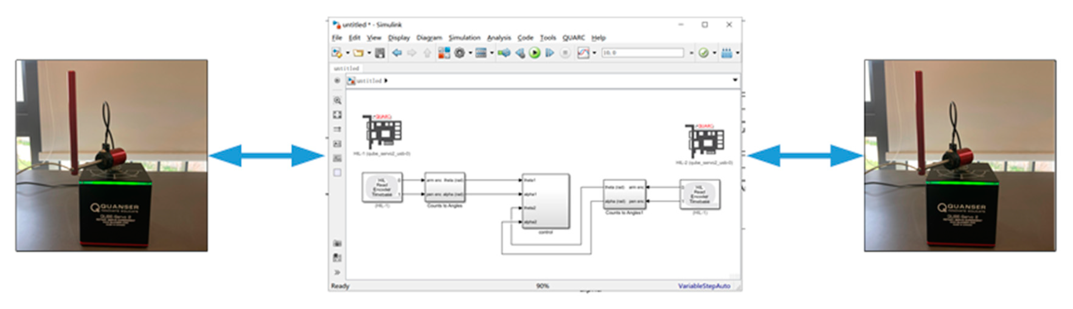
The organization of the paper is as follows. After the introduction section, the data-driven state prediction algorithm is introduced in Section 2. Based on the prediction model, a residual-triggered fault classification technique is proposed in Section 3. Section 4 presents the experimental results in a twin rotational inverted pendulum system with leader-follower mechanism. The paper is ended by Section 5 with the conclusion and future researches.

2. Data-Driven State Prediction for Multi-Agent System

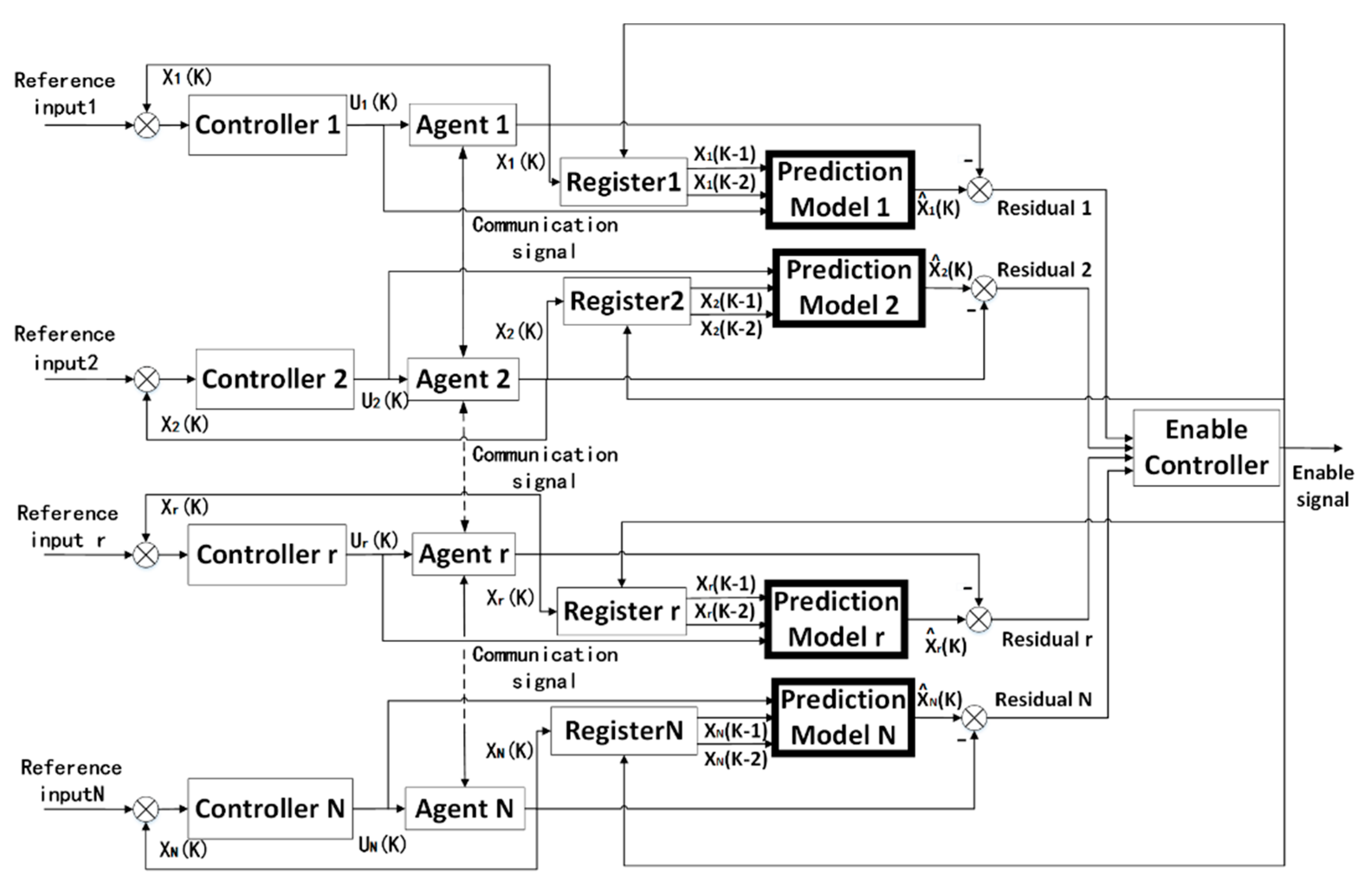
In this section, we introduce the establishment of a neural network model to predict the state of a multi-agent system with unknown communication. To be precise, the controller of each agent and communication protocol among the agents are pre-designed to guarantee the performance of a multi-agent system (i.e., consensus and robustness) in a fault-free case, and the design of the controller and communication is not of concern in this paper. The physical models of the agents are unknown or highly nonlinear. Moreover, the communication protocol is internal to the system, but not available for the prediction model.

The diagram of the prediction model for the multi-agent system is shown in Figure 1.

In Figure 1, $X_r$ and $U_r$ represent state and control input of agent $r, r=1,2,\dots N$, and $N$ is the number of agents; $K$ represents the time of $KT$, where $T$ is the sampling time; $K-1$ and $K-2$ represent the time of $\left(K-1\right)T$ and $\left(K-2\right)T$, respectively, ${\widehat{X}}_r\left(K\right)$ is the prediction of $X_r\left(K\right)$. Firstly, the state of each Agent $r$ is recorded in the corresponding Register $r$ at the past two sampling times, namely $X_r\left(K-1\right)$ and $X_r\left(K-2\right)$ are obtained. Then, $X_r\left(K-1\right)$, $X_r\left(K-2\right)$ and control input of Agent $r$ at current time $U_r\left(K\right)$ are used to train the Prediction Model $r$. The output of the prediction model is the predicted state at the current time ${\widehat{X}}_r\left(K\right)$. By comparing the real state $X_r\left(K\right)$ and the predicted state ${\widehat{X}}_r\left(K\right)$ $\mathrm{Residual}r={\widehat{X}}_r\left(K\right)-X_r\left(K\right)$ can be generated. The residual values are sent into Enable Controller, which is responsible for deciding whether the residual exceeds the threshold. To be precise, when it exceeds the threshold, it is recognized that there is a fault in the system. At this time, the enable signal stops the prediction model and triggers fault diagnosis algorithms, which will be presented in Section 3.

The enable control algorithm is described as follows:

$$\begin{array}{c}\mathrm{if}\mathrm{Residual}1>{\beta }_1\mathrm{or}\mathrm{Residual}2>{\beta }_2\mathrm{or}\dots \mathrm{Residual}\mathrm{N}>{\beta }_{N}enable=1\hfill \\ \mathrm{else}\hfill \\ \hfill enable=0\end{array}$$

where, ${\beta }_r$ represents the residual threshold of Agent $r$, $enable$ is the output of Enable Controller.

Remark 1.

It should be mentioned that communication among agents is not used in the prediction model. The “unknown communication” in this paper means the communication is internal to the MAS, but cannot be used in the prediction/fault diagnosis. Moreover, the controllers are predesigned for the MAS, which is not under concern in this paper.

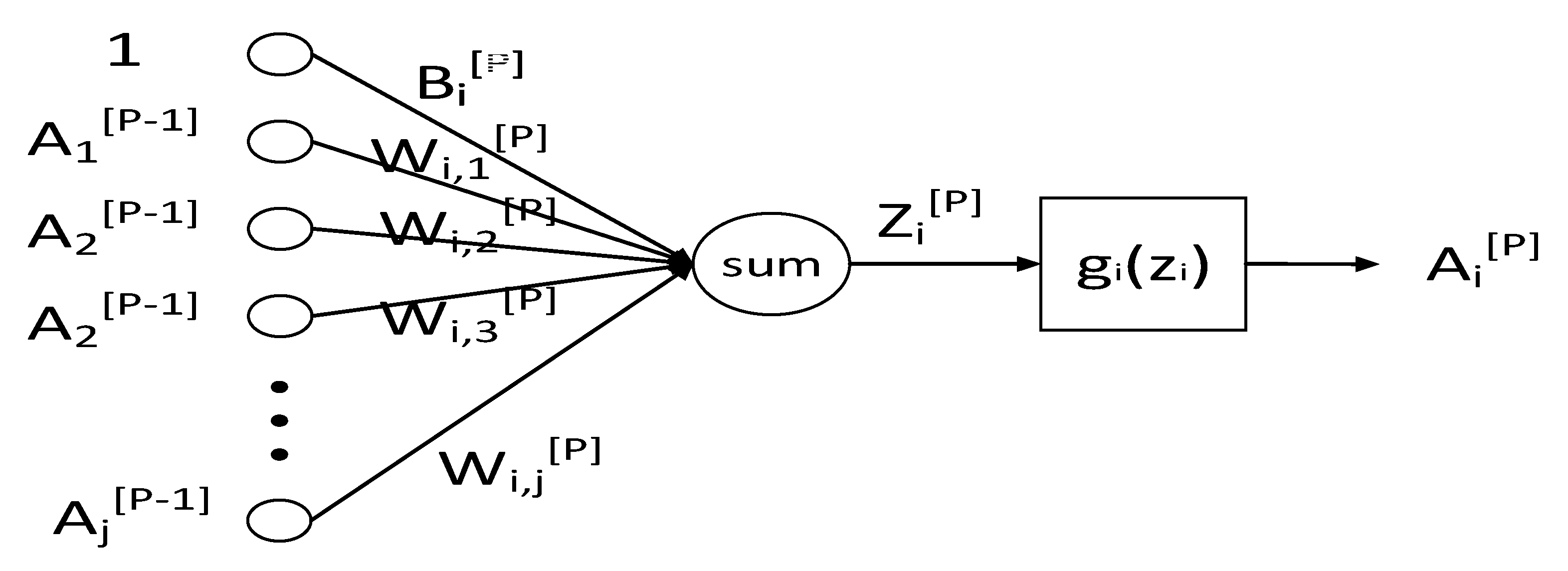
The network structure used to build the prediction model is the back propagation (BP) neural network, which is known as a multilayer feedforward neural network trained by error back propagation algorithm. It can learn and store a large number of input–output pattern mapping relations without concrete mathematical functions. A neural network is composed of a number of neurons, and the BP neural network of a single neuron for predicting the concerned model is shown in Figure 2.

In the diagram, $W_{ij}^{\left[P\right]}$ and $B_i^{\left[P\right]}$ represent the weight parameter and bias parameter between hidden layers, respectively; $P$ represents the number of current layers; $i$ and $j$ represent the number of current nodes in the current layer and the number of current nodes in the upper layer, respectively. $Z$ represents the input of the neuron and the output of the weighted multiplication summation. A represent the input or output of the neuron. Where:

$$Z^{\left[P\right]}=W^{\left[P\right]}·A^{\left[P-1\right]}+B^{\left[P\right]}.$$

(1)

The hidden layer takes the Tansig function as the excitation function $g_1\left(x\right)$, where:

$$g_1\left(x\right)=\frac{2}{1+e^{-2x}}-1.$$

(2)

The reason for using the Tansig function is that the training data changes periodically in $\left[-1,1\right]$. Using Tansig can accelerate the decline of training gradient.

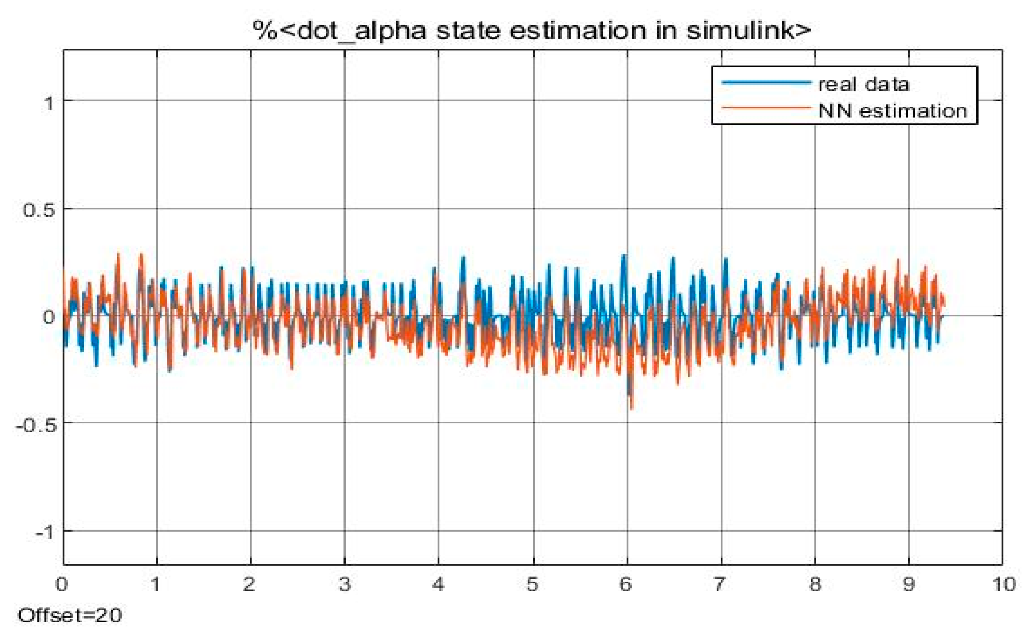
The output of the neural network is the predicted value of system state ${\widehat{X}}_r\left(K\right)$ in a fault-free scenario. Therefore, the output layer uses the Purelin function as the activation function, which is defined as $g_2\left(x\right)$, and

$$g_2\left(x\right)=x.$$

(3)

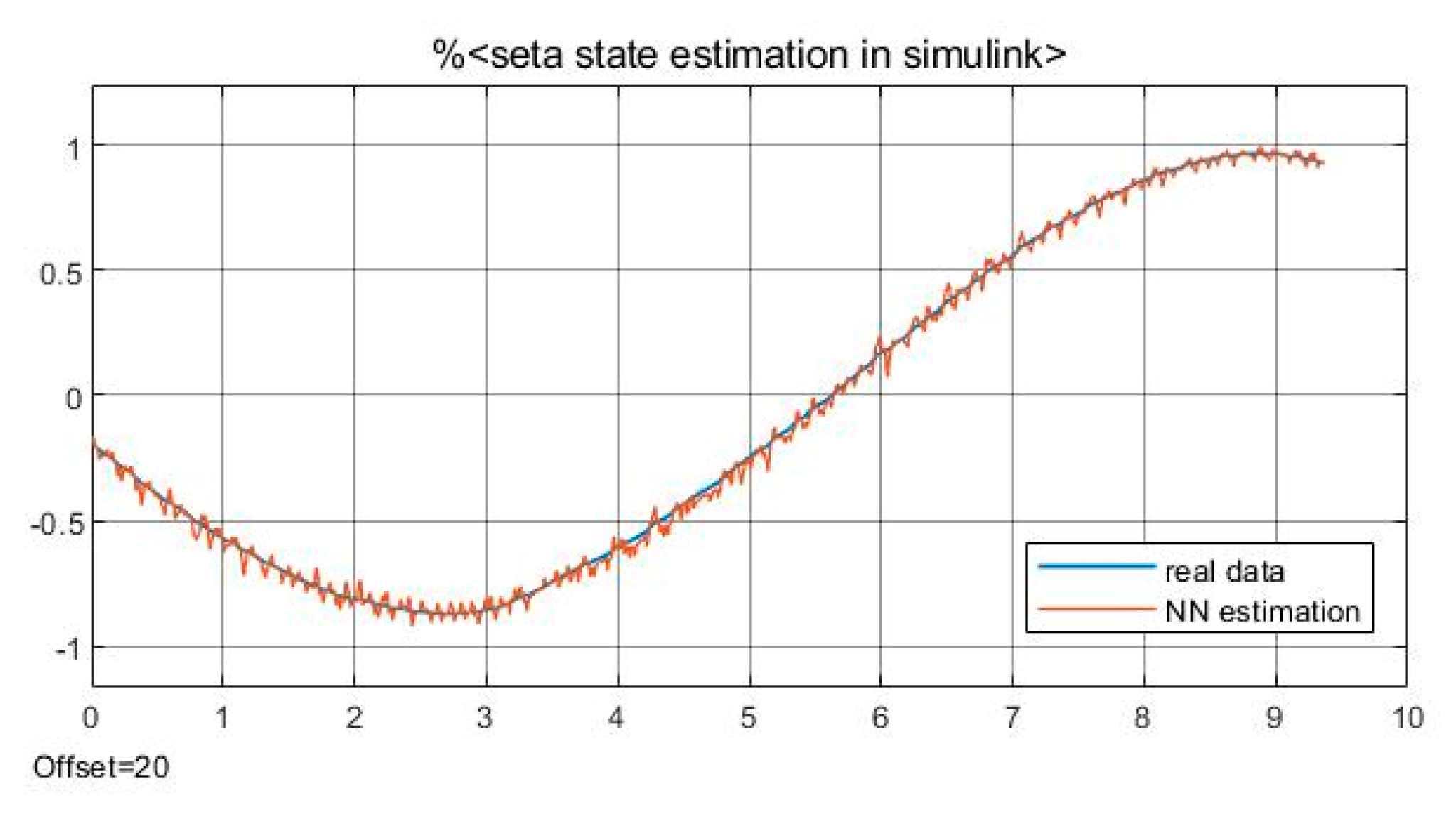
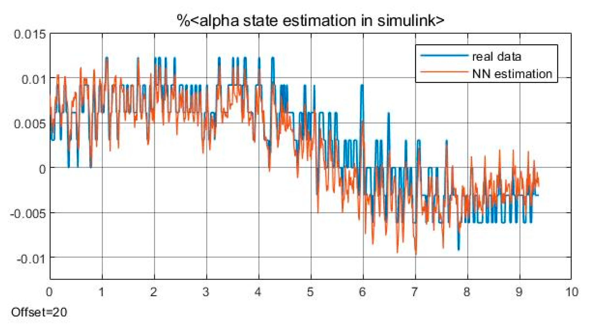
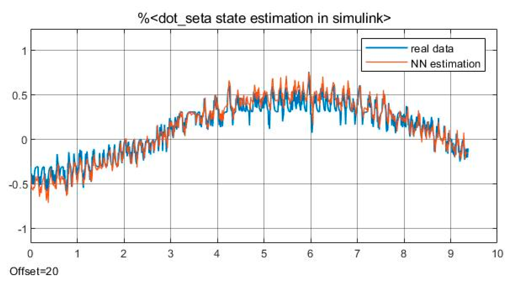
The predicted state ${\widehat{X}}_r\left(K\right)$ is compared with the actual system state $X_r \left(K\right)$ and the network topology structures and training parameter should be designed to make ${\widehat{X}}_r\left(K\right)$ closed to $X_r \left(K\right)$.

In the healthy state, the residual between ${\widehat{X}}_r\left(K\right)$ and $X_r \left(K\right)$ is convergent. However, when the system is in the fault state, the residual will exceed the threshold. At this time, it is deemed to be in the fault state and start fault diagnosis.

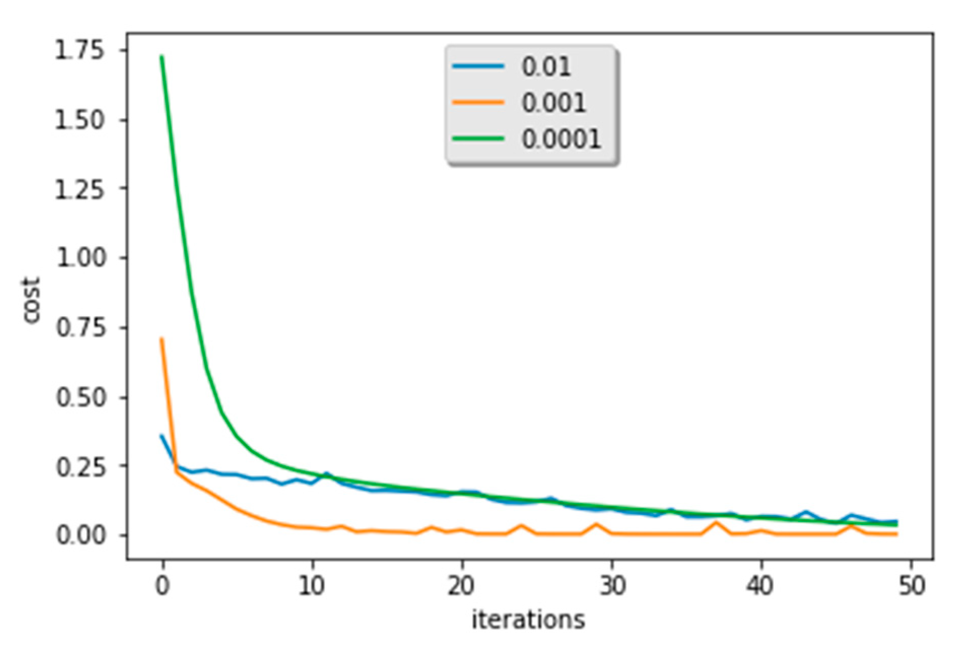
Root mean square error (RMSE) between the predicted value and the actual value is used as the evaluation standard of the prediction accuracy. In BP neural network, the gradient descent is used to update the $W_{ij}^{\left[P\right]}$ and $B_i^{\left[P\right]}$ until the RMSE between ${\widehat{X}}_r\left(K\right)$ and $X_r \left(K\right)$ is locally minimum. As a result, the optimal weight and bias parameters of the neural network are calculated.

There are a variety of network structures and learning rates. In order to obtain optimized performance of the state prediction, RMSEs of different hierarchical structures under the same training parameters and the same training time are generated and compared. Generally speaking, smaller the RMSE value indicates better training performance, however, the generalization capability should also be considered to avoid over fitting. Accordingly, the network structure can be determined. Subsequently, learning rates are determined by comparing their accuracy with the selected network structure.

Then, the developed state prediction model can be implemented to a real-time system to predict the state in absence of fault. By comparing real state and the predicted health state, a residual signal can be generated. This residual signal can indicate whether a fault occurs, and if the residual signal excesses a threshold, it triggers a fault classification mechanism, which is designed in Section 3.

3. Sensor Fault Classification

The fault of one sensor may lead to the fault of the whole system [23]. Therefore, it is very important to diagnose the fault of the sensor.

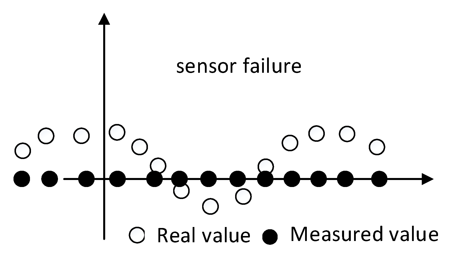
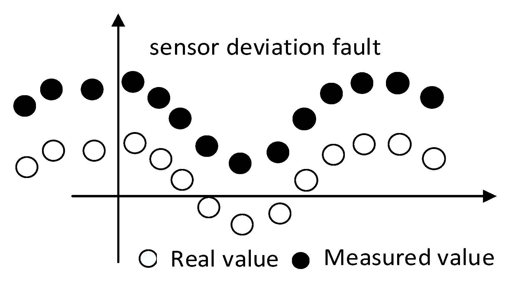
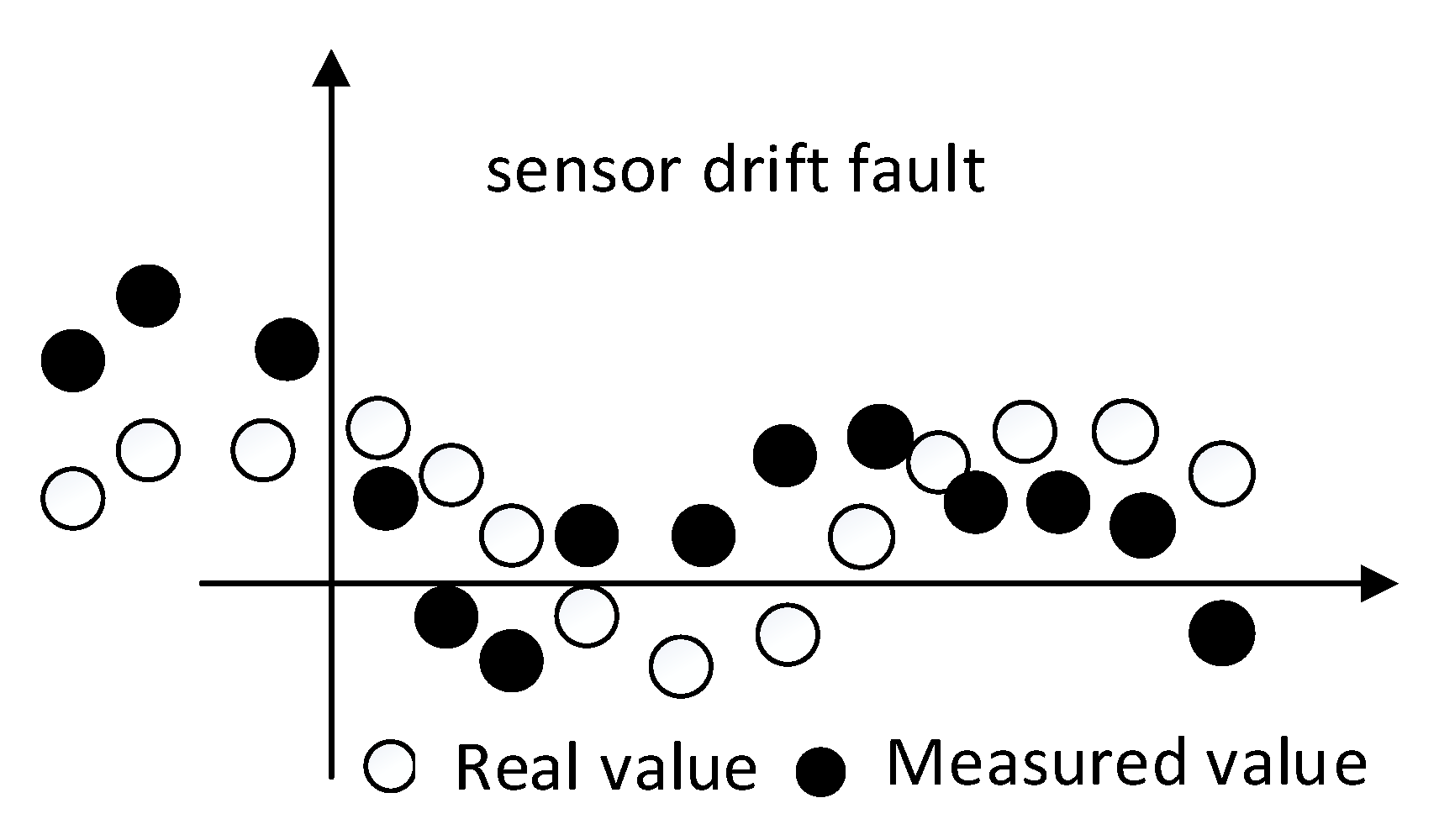
In this section, a data-driven sensor fault detection and classification technique is presented. Three typical sensor faults are under consideration: zero-output fault, drift fault, and deviation fault. Figure 3, Figure 4 and Figure 5 are schematic diagrams of the three types of sensor faults. Moreover, the three types of faults can exist in different sensors and different agents. The objective of this section is to use a neural network classifier to identify and locate different types of faults.

Specifically, the zero-output sensor fault [24] is molded as:

$$f_s\left(t\right)=\{\begin{array}{c}0, t<t_0 \\ -y\left(t\right), t\ge t_0\end{array}$$

(4)

where $f_s\left(t\right)$ represents sensor fault, $t_0$ denotes the time that a sensor fault occurs, $y\left(t\right)$ is the real system output. In engineering, it is easy to occur when the signal is open circuited. A deviation fault is molded as:

$$f_{de}\left(t\right)=\{\begin{array}{c}0, t<t_0 \\ d, t\ge t_0\end{array}$$

(5)

where $f_{de}\left(t\right)$ represents deviation fault and $d$ is a bounded constant. The deviation fault is easy to appear in the current or voltage sensor [25]. A drift fault is molded as:

$$f_{dr}\left(t\right)=\{\begin{array}{c}0, t<t_0 \\ n\left(t\right), t\ge t_0\end{array}$$

(6)

where $f_{dr}\left(t\right)$ represents drift fault and $n\left(t\right)$ is an irregular bounded disturbance signal, which is a sensor noise (due to the influence of external environment and internal factors of the sensor) [26].

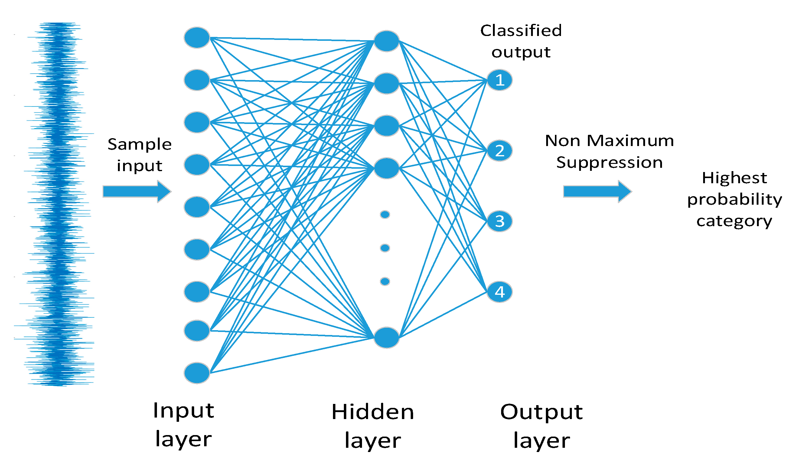
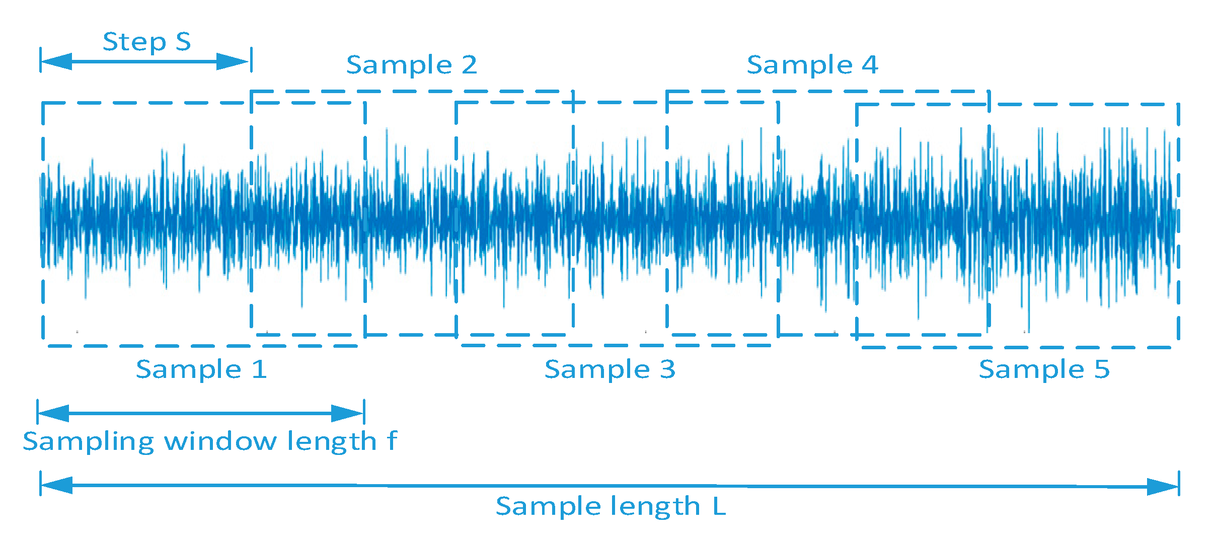
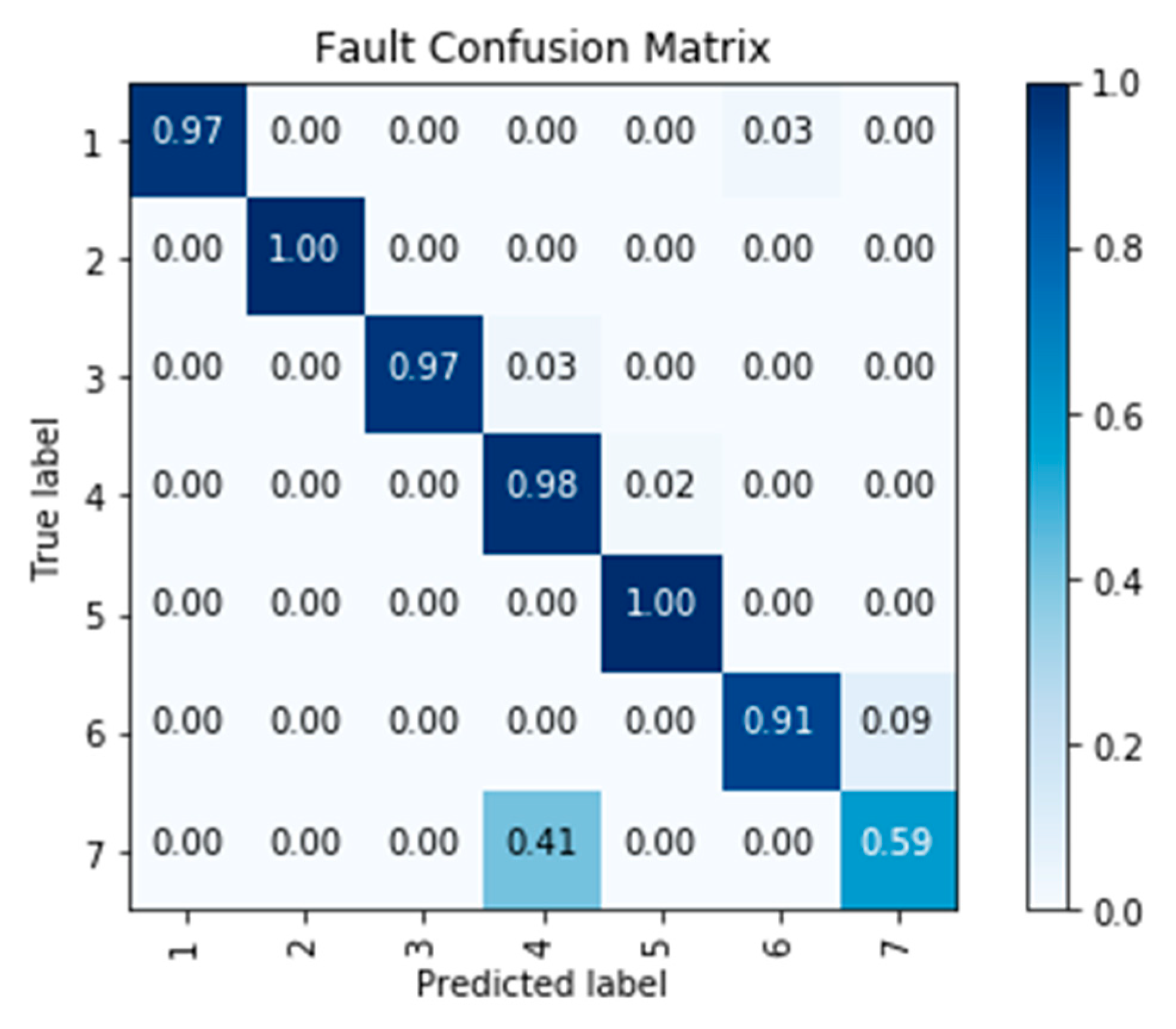
The data used to train the classifier is $X_r\left(K\right)$. The procedure to select an appropriate network structure and learning rate is the same with state prediction. The output of the classifier is the probability of each fault category, therefore, the last output layer activation function is replaced by the Softmax function. Through non-maximum suppression, the original network output is fuzzed, and the fault type and location with the highest probability can be determined. The network structure diagram of a fault classification model can be found in Figure 6.

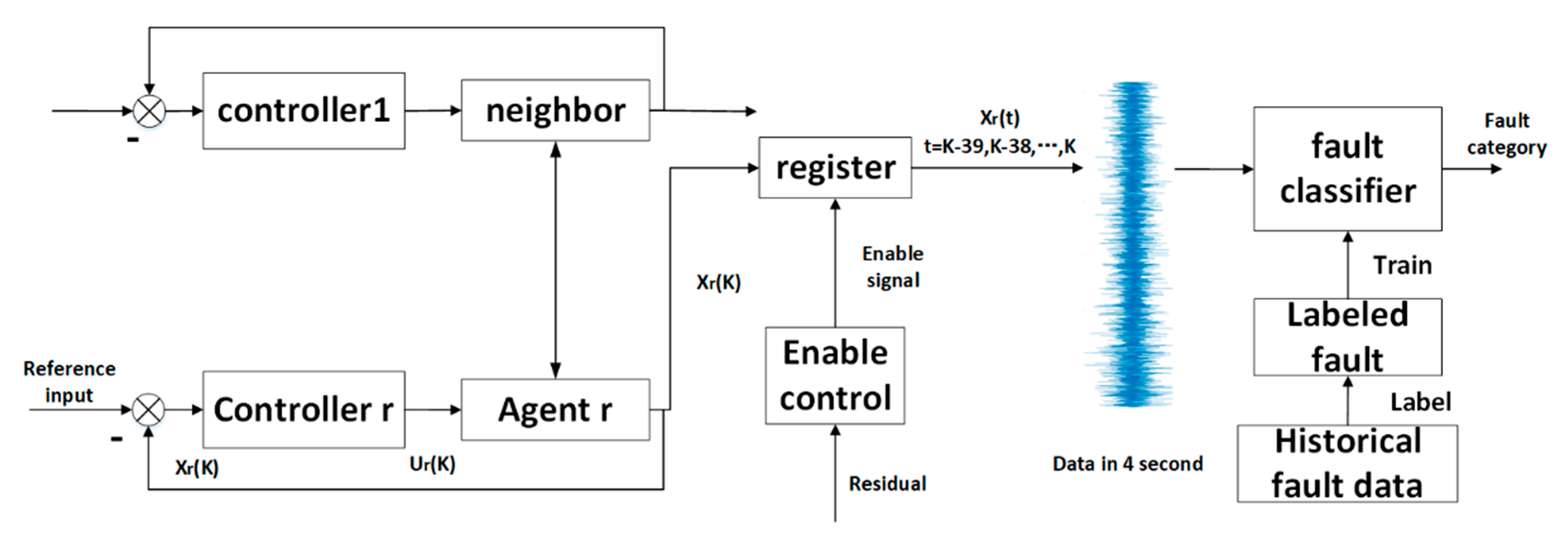
In the fault classification model, the amount of network input data can be large. Identification of such an amount of data in real-time brings a challenge to the computation ability. As a result, a triggering mechanism is designed to active the identification. Specifically, the prediction model introduced in Section 2 is implemented in the system to predict the system state and output in absence of fault. By comparing the predicted healthy output and the measured output, which can be abnormal in the case of sensor faults, a residual signal can be generated. When a sensor fault occurs, the residual signal exceeds the threshold, and the fault diagnosis model of the neural network is triggered to identify and locate the fault types. The state prediction triggered fault classification mechanism is illustrated in Figure 7.

When the residual in Figure 1 is greater than the set threshold, Enable Controller sends an enable signal to the register of fault classifier in Figure 7, and the register starts to record the abnormal state data of the agent for 4 s. The stored data is then sent to the fault diagnosis network. The fault diagnosis network is obtained by labeling historical fault data and off-line supervised learning. The diagnosis model can classify the faults in agent $r$ and its neighbor through the output of agent $r$. Moreover, communication is not utilized in the fault classifier.

4. Experimental Results

4.1. System and Fault Description

In this section, the designed data-driven state prediction and the sensor fault classification techniques are implemented to the collaborative system to verify the effectiveness. We use two Quanser Servo 2 rotating inverted pendulum hardwares to build a multi-agent system with internal communication. The communication protocol is a leader-follower mechanism. The inverted pendulums transfer sensor data to Matlab Simulink in real-time through USB, and the control protocol is pre-designed in Simulink. The specific hardware-in-the-loop control diagram is shown in Figure 8. There are four states of each agent, which are introduced in

Table 1. Parament and meaning.

Parameter	Representative Meaning
$\theta$	Horizontal displacement of inverted pendulum
$\alpha$	Vertical displacement of inverted pendulum
$\dot{\theta }$	Horizontal velocity of inverted pendulum
$\dot{\alpha }$	Vertical velocity of inverted pendulum

.

It is assumed that the faults occur in the horizontal displacement sensor, and seven scenarios of faults are under investigation: fault-free, leader’s zero-output sensor fault, leader’s sensor deviation fault, leader’s sensor drift fault, follower’s zero-output sensor fault, follower’s sensor deviation fault, and follower’s sensor drift fault.

Remark 2.

The equipment is working in a real laboratory environment. Thus, the data collected is subjected to noises/disturbances due to equipment noises, environment noises, data conversion uncertainties, etc. On the other hand, drift fault can also be regarded as disturbances with relatively big amplitude. In order to avoid alarm by acceptable noises in the data, we select the threshold parameters for the enable control as ${\beta }_1={\beta }_5=0.5; {\beta }_2={\beta }_6=0.006; {\beta }_3={\beta }_7=0.3; {\beta }_4={\beta }_8=0.25$.

4.2. Data Acquisition and Data Expansion

The data acquisition of the system is carried out through Simulink, then a hardware-in-the-loop experiment can be implemented. The data sampling is carried out according to the sampling time of 0.005 s. Due to the limited storage capacity of MATLAB, 29 s of effective data can be collected in each experiment.

In order to further improve the generalization ability of the model, a large number of data is needed to train the neural network. Nevertheless, it is often impossible to collect sufficient data in reality. Therefore, this paper is motivated to employ sliding window data sampling to complete data amplification. As shown in Figure 9, if the length of the sampling window is $\mathit{f}$, the moving step of the sampling window is $\mathit{S}$, and the total length of the data is $\mathit{L}$, the number of data $\mathit{n}$ can be obtained as:

$$\mathit{n}\mathbf{=}\mathbf{\left[}\frac{\mathit{L}\mathbf{-}\mathit{f}}{\mathit{S}}\mathbf{\right]}$$

(7)

The original data is collected from each fault during 29 s, and the sampling time is 0.005 s. The total length of the signal is 5800 sampling points ($L=5800$). By selecting 800 sampling points ($f=800$) with the length of the sampling window and one sampling point in step ($S=1$), 5000 groups of data ($n=5000$) in each fault state can be obtained, and a total of 35,000 groups of 7 kinds of fault scenarios can be obtained. Compared with the original method with 40 sampling window length, the amount of data is increased by 114.28 times.

4.3. Experimental Results and Analysis

4.3.1. Neural Network-Based State Prediction

The historical healthy and stable operation data are selected as the network training input of state estimation. The training process is offline. The process of recognition is to connect the offline trained model into the system to complete online prediction.

Neural network models with different hidden layer nodes, learning rate and momentum factor, and the training effect of the final network are compared in

Table 2. Performance comparison of neural networks with different parameter structures.

Number of Hidden Layer Nodes	Learning Rate	Momentum Factor	RMSE
8/4	0.001	0.99	0.0623
	0.001	0.95	0.0652
	0.010	0.99	0.0641
	0.010	0.95	0.0627
15/4	0.001	0.99	0.0598
	0.001	0.95	0.0592
	0.010	0.99	0.0604
	0.010	0.95	0.0597
15/8/4	0.001	0.99	0.0579
	0.001	0.95	0.0553
	0.010	0.99	0.0517
	0.010	0.95	0.0571

, where the performance of state prediction is evaluated by measuring RMSE.

The basic structure of the BP shallow neural network for predicting the concerned model is shown in the Figure 10.

From Table 2, we can notice that the most accurate state prediction model is the three-layer neural network with RMSE equal to 0.0517. The structure of the network is 15/8/4 from input to output in turn. However, the neural network will appear over the fitting phenomenon when the model is too accurate, which can cause the divergence of the system when processing the data that does not appear in the training set. To be precise, the data that does not appear in the training set refers to the data that appear in normal operation but that is not in the training set. Identifying these data requires the network to have a certain generalization ability. As a result, this paper selects a two-layer neural network with the middle accuracy. Its parameters are: a learning rate of 0.001, momentum factor of 0.95, and layer series from input to output of 15 and 4.

Figure 11, Figure 12, Figure 13 and Figure 14 compare actual states and predicted states. As shown in the results, the neural network can accurately predict the full states of an inverted pendulum, which can be used as a healthy signal and compared with the actual output to monitor whether the system is under fault-free case or not. In case of sensor faults, the residual signal can be generated immediately to trigger the fault identification and classification process.

4.3.2. Fault Classification

Through the method introduced in Section 3, we can build the neural network for fault classification. The training data is divided into two parts: 70% and 30%. Seventy percent of the data is used to train the network, update the model weight parameters, and the remaining 30% is used to evaluate the model performance. According to the fault detection of the horizontal displacement sensor of the leader-follower system, the faults can be divided into seven types.

We stipulate that all collection time of data is 29 s and the sampling time is 0.005 s. Thus, 5800 sampling points can be collected within 29 s. The cycle time of inverted pendulum motion is 7 s, and 1400 sampling points need to be collected when we use a sampling time of 0.005 s. If there are $m$ sensors in the system, there are $m\times 1400$ neural network inputs, which require a lot of operation for training. However, the calculation ability of software is limited. In order to reduce data calculation, we expend the sampling time of the sliding window after data expansion to 0.1 s. The length of the sliding window is 4 s (40 sampling points), which is more than half a cycle of the system. According to Formula (7), the number of total data is 5000. Because the data acquisition is carried out just when the fault occurs, the data of the first 40 minimum sampling points (0.2 s) are filtered as the signal delay. All subsequent data segments contain the fault characteristic information, except that the fault characteristics of some faults only last for a few seconds. In this scenario, the whole data acquisition time cannot be filled, and the edges of the data need to be filtered to retain the parts with fault characteristics. For the fault requiring edge screening, several groups of fault data shall be collected to supplement 4960 groups of data. The parameter is provided in

Table 3. The type of faults and category label.

Sample Type	Sample Length	Number of Sample	Category Label
leader and follower work normally	40	4960	1
leader’s zero-output sensor fault	40	4960	2
leader’s sensor deviation fault	40	4960	3
leader’s sensor drift fault	40	4960	4
follower’s zero-output sensor fault	40	4960	5
follower’s sensor deviation fault	40	4960	6
follower’s sensor drift fault	40	4960	7

:

In order to enhance the result, we did experiments with different number of nodes in different hidden layers, and the fault classification performances are compared in

Table 4. The train set result of different bp model (%).

Run No.	BP-25-12	BP-50-25	BP-50-12	BP-80-50	BP-80-25	BP-80-12
1	98.50	98.15	98.65	97.32	98.71	99.49
2	97.96	98.85	98.37	98.69	97.96	97.73
3	96.49	97.32	96.75	99.09	99.01	98.00
4	99.35	97.98	98.25	99.06	99.06	98.35
5	98.53	96.50	95.43	97.32	98.42	99.11
Mean	98.16	97.76	97.49	98.30	98.63	98.54
Std	1.0603	0.8902	1.3683	0.9048	0.4552	0.7435

and

Table 5. The test set result of different bp model (%).

Run No.	BP-25-12	BP-50-25	BP-50-12	BP-80-50	BP-80-25	BP-80-12
1	84.72	81.40	85.58	79.91	82.51	71.92
2	77.13	84.12	81.31	79.11	88.78	79.54
3	79.56	80.97	83.83	84.72	87.29	70.26
4	76.50	84.12	91.53	83.17	87.46	81.14
5	89.44	75.33	81.74	79.91	90.87	80.37
Mean	81.47	81.19	84.80	81.36	87.38	76.65
Std	5.5061	3.5917	4.1348	2.4410	3.0770	5.1370

. To be precise, Table 4 records the average accuracy and standard deviation of the training set of the network model under the same learning rate but with different random initialization conditions and different number of nodes. Accordingly, the average value accuracy and standard deviation of test set are shown in Table 5. Through the above experiments, we can find a network structure with the highest accuracy, which is achieved when the number of the hidden layers is 80-25, As a result, we chose the 80-25 hidden layer structure.

After the network structure is determined, the accuracy of the model can be further enhanced by selecting the appropriate learning rate. Figure 15 records the number of iterations and loss function values corresponding to different learning rates, and the accuracy is compared in

Table 6. The result of different learning rate (%).

Learning Rate $\mathsf{\alpha }$	0.01	0.001	0.0001
Train accuracy	98.42	100	99.56
Test accuracy	90.87	88.38	91.81

. From Figure 15 and Table 6, the gradient decreases the fastest when the learning rate is 0.001. However, the corresponding test accuracy is only 88.38%. This is due to the overfitting phenomenon in deep learning. From overall consideration, the learning rate is determined as 0.0001, where the gradient descent speed is the second fastest, and the test accuracy is the highest.

Until now, the network structure and learning parameters are determined. Then, the test set of different fault scenarios is input to the determined neuro-network-based fault classifier, and the results are illustrated in

Table 7. The result of different fault type (%).

Label	1	2	3	4	5	6	7
Accuracy	97.2	100	96.8	98.4	100	91.6	58.72

. It can be seen that the classifier can achieve 100% recognition rate for types 2 and 5, and more than 90% recognition rate for types 1, 3, 4, and 6. The recognition rate of type 7 is only 58.72%, which is not ideal. In order to show the performance of BP neural network algorithm on sensor fault diagnosis of leader-follower fault system, the fault misclassification matrix is drawn in Figure 16.

In Figure 16, the coordinate values from 1 to 7 are the label numbers in Table 3, representing different fault types of the leader-follower system. The number in the shadow is the number of actual sample tags that match the predicted sample tags. It shows that the probability of misclassifying most types of faults is not big. However, the error rate of type 7 is significant, and it cannot be distinguished from type 4. The occurrence of misclassification is due to the similar characteristics between the corresponding types. For example, types 4 and 7 have no significant difference in amplitude characteristics, but their frequency characteristics are different. Moreover, the amplitude is small, namely, drift fault is like disturbance, which is challenging for classification.

4.4. Discussions

4.4.1. Delay of Fault Diagnosis

The developed state prediction is implemented in real-time, and there is nearly no delay. When the state varies fast, tracking errors exist, and this phenomenon is general in many estimation/prediction problems. The tracking errors in the experiments is small and acceptable. When we label fault types, the faults occur for a period of time, hence, a complete fault feature is recorded in data sequence during this period. When the residual triggers the fault classifier, there is a period of delay such that complete data of the fault can be stored in the register. It generally takes 2–3 s for complete fault features to appear. The fault diagnosis module can identify the corresponding fault only after a complete fault feature is recorded in the register. Therefore, the delay is also acceptable.

4.4.2. A Limitation of Performance and Further Research

Through the above, we can find that the BP network model is more accurate for amplitude type feature recognition, but not ideal for frequency type feature recognition. Because there are different amplitude characteristics and frequency characteristics in the seven types of faults. Under limited calculation ability of the software, amplitude features can be effectively preserved, however, the frequency characteristics will be partially lost with the increase of the sampling interval. Therefore, faults with similar amplitude but different frequencies, namely drift faults, are difficult to be identified. This leads to a decrease in recognition accuracy. In future research, an alternative network will be investigated to classify faults with the same and small amplitude but a different frequency.

It can be noticed that the developed state prediction and fault classification techniques are distributed, namely the techniques are potential to be generalized in many MASs where the number of agents can be large. In addition, the mathematical model is not required, and only input and output data is utilized in the methods. Therefore, the methods are extendable for many other MASs where the type of agents can be diverse, such as cooperative manipulators (4–6 freedoms), cooperative unmanned aerial vehicles, etc.

5. Conclusions

This research presents a data-driven state prediction and fault classification method by the BP neural network model. The main contribution is to establish a state prediction model for a multi-agent system with unknown communication, and a residual-triggered fault classifier for sensor faults. The developed techniques are implemented in a real physical system. Specifically, for the leader-follower system with communication coupling, the fault diagnosis of the leader can be achieved by observing the follower. RMSE can reach 0.0592 for the state estimation of a leader-follower system. In terms of fault diagnosis, observing the follower to realize the fault diagnosis of the leader is an innovation. Investigation of data-driven state prediction and residual-triggered fault classification of multi-agent systems with unknown communication is a new topic; identification of fault in one agent only through data of its neighbors is a contribution to the distributed fault problem. In the future, more fault types will be considered, such as actuator faults or communication faults. Moreover, improving the fault recognition rate is also in our further research.