
A Numerical Study on Axial Pump Performance for Large Cavitation Tunnel Operation


1
Department of Naval Architecture & Ocean Engineering, Mokpo National University, Jeollanamdo 58554, Korea
2
Department of Naval Architecture & Ocean Engineering, Chungnam National University, Deajeon 34134, Korea
3
Daewoo Shipbuilding & Marine Engineering Co., Ltd., Siheung 15011, Korea
*
Author to whom correspondence should be addressed.
Processes 2021, 9(9), 1523; https://0-doi-org.brum.beds.ac.uk/10.3390/pr9091523
Submission received: 27 July 2021
/
Revised: 22 August 2021
/
Accepted: 24 August 2021
/
Published: 27 August 2021
(This article belongs to the Special Issue Theoretical and Numerical Marine Hydrodynamics)
Abstract
:In this paper, a numerical investigation was carried out on the performances of a designed axial flow pump for a large cavitation tunnel. From this, the flow characteristics, force, and torque performance of the axial flow pump were investigated, and the rotating speeds of the impeller satisfying the test section speed performances required in the large cavitation tunnel were estimated. The axial flow pump was modeled such that the impeller, stator, and nacelle were located in a cylindrical tunnel. The calculations were carried out for incompressible steady-state turbulent flow considering the impeller rotating. The performance of the pump was confirmed, finding that the head gain was caused by the pressure jump downstream of the pump. The performance of the stator was confirmed to be good enough to refine the tangential flow due to the impeller rotating. To investigate the operating performance of the large cavitation tunnel, the head loss of the entire tunnel without the pump was obtained from a numerical analysis. The operating points were estimated from the specific speed–head coefficient curves, and it was found that the present numerical results were in good agreement with the experiments.
1. Introduction
A large cavitation tunnel is a circulation water channel facility capable of controlling pressure and speed to perform cavitation experiments for commercial ships, battleships, submarines, and so on. In order to reduce the scale effect, as the size of the model ship increases, the size of the tunnel test section also increases, and the cavitation tunnel also becomes enlarged. Accordingly, the head loss of the tunnel increases, and since a large amount of water circulates in the closed tunnel, it becomes very important to supply enough energy to circulate water. In order to perform a cavitation experiment, it is essential to control the flow speed in the test section, and such a time, the relationship between the pump and the flow speed of the test section should be identified, and the correct operating point should be selected. For this, it is necessary to know in advance whether the tunnel operation is possible with the pump performance.
In 2020, Daewoo Shipbuilding and Marine Engineering built a large cavitation tunnel (DLCT) at DSME Siheung R&D Center in Korea to conduct various cavitation experiments. An axial flow pump was installed for this DLCT operation. The pump of a large cavitation tunnel generally employs an axial flow pump. It is a major noise source that can increase background noise; thus, it should have low vibration. Additionally, it should be designed so that cavitation does not occur under any operating conditions. The number of blades is increased due to problems such as the noise of the pump, and more than 7 impeller blades have been adopted in the existing large cavitation tunnels, such as LCC, HYKAT, FNS, and LCT [1,2,3]. In the case of impeller cavitation, large cavitation tunnels usually have a height of about 20 m, so that there is almost no cavitation problem due to high hydrostatic pressure.
On the other hand, research on the pumps installed in cavitation tunnels has been conducted experimentally and numerically, mainly for centrifugal pumps applied to small- and medium-sized tunnels [4,5,6,7]. A centrifugal pump has a relatively small capacity and is applied in various fields. However, studies on large-capacity axial flow pumps are rarely found. Performance verifications or studies through model tests have been mainly carried out, and there are some studies involving experiments and numerical analyses [8,9,10,11]. Since the axial flow pump of a large cavitation tunnel is quite large, sufficient information must be provided at the design stage to design a pump with excellent performance. In particular, since the performance of the pump is directly related to the performance of the test section, examination at the design stage is very important to achieve the operational goal of the tunnel. In this process, performance estimation through experiments is the best way, but experiments are accompanied by many difficulties in terms of time and cost. Therefore, the use of numerical analysis is more efficient method.
Recently, numerical analysis has been used in a variety of fields and has given reasonable results qualitatively and quantitatively. In the field of shipbuilding and marine engineering, the range of applications is wide enough to be used not only in research but also in design. Therefore, it is possible to use numerical analysis in the design of the axial flow pump, and it would be reasonable to conduct a performance evaluation through numerical analysis before model tests or trial tests.
In this study, numerical analysis is used to examine the performance of an axial flow pump for a large cavitation tunnel for DSME (DLCT). Numerical analyses were performed on an axial flow pump consisting of an impeller, stator, and nacelle located in a cylindrical tunnel. From this analysis, the performance of the pump and flow characteristics were investigated. Additionally, to confirm whether the requirements of flow speed of the test section were satisfied, the operating points were obtained from the head gain of the pump and the head loss of a large cavitation tunnel. The organization of this paper is as follows. Section 2 briefly describes the shape of the axial flow pump as well as the large cavitation tunnel where the pump is mounted. In Section 3, numerical analysis techniques and grid systems are presented. In Section 4, the numerical results of the pump performance are presented, and the performance of the impeller and the stator is discussed. In Section 5, the head loss of large cavitation tunnel for the head identity is estimated through numerical analysis, and the numerical results of the head loss according to the speed of the test section are presented. In Section 6, the pump performance in the given test section flow speeds is estimated by the head identity from the head gain of the pump and the loss head of the large cavitation tunnel. Finally, conclusions are given in Section 7.
2. Geometry
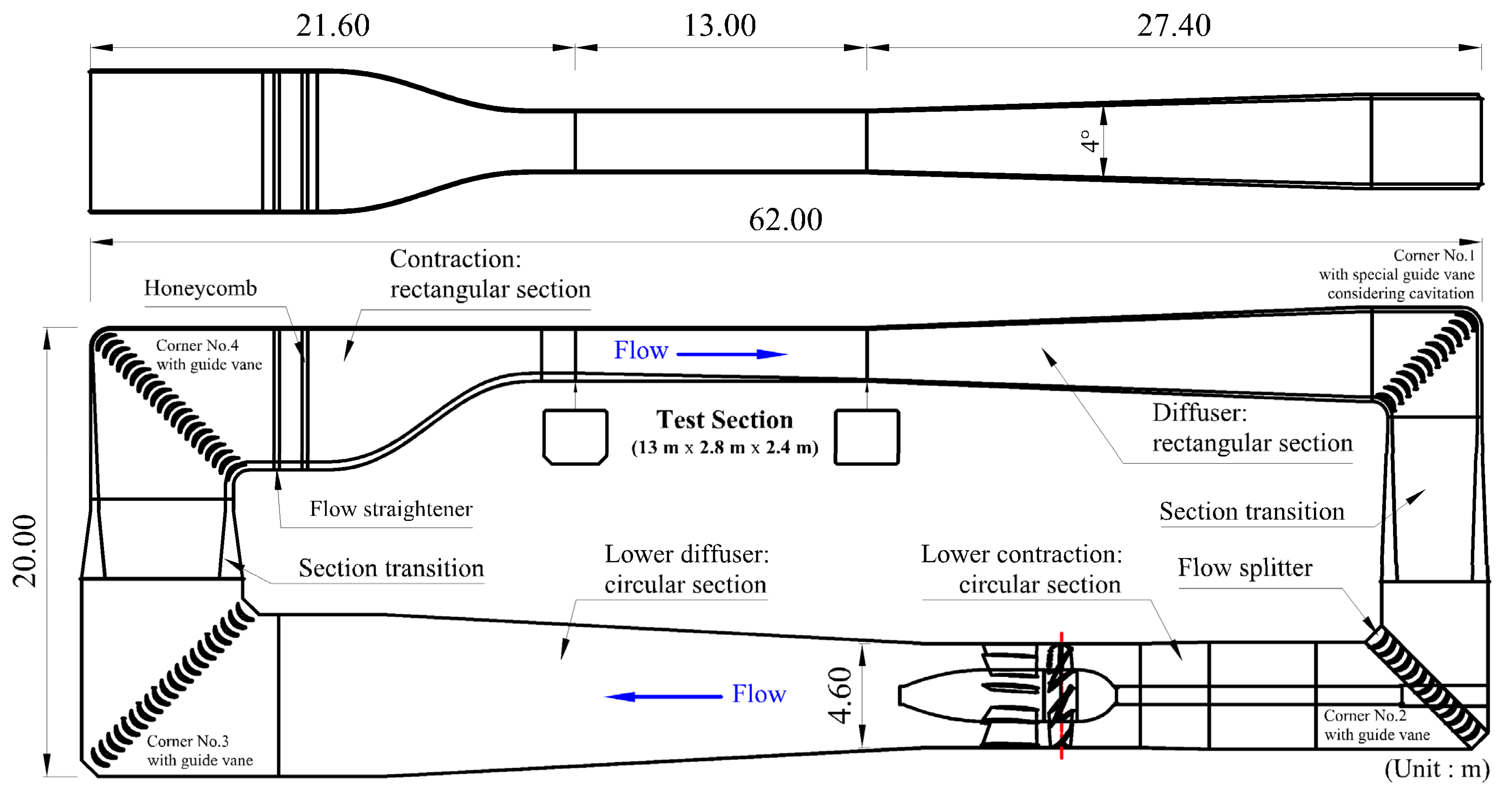
Although this study focused on the axial pump of the DSME large cavitation tunnel (DLCT), the tunnel is briefly introduced. The layout of the DLCT is shown in Figure 1. The overall length of the DLCT is 62 m and the height is 20 m. The test section is 13 m in length, 2.8 m in width, and 2.4 m in height with the chamfered corner, and the DLCT is equipped with a flow settling chamber that consists of flow straightener and honeycomb. In addition, there are guide vanes in the four corners for circulation of the flow, and since it is necessary to reduce the flow speed by increasing the cross-sectional area to decrease the power required to circulate water, there is a contraction and diffuser before and after the test section. The area ratio of the contraction is 6.14 and that of the diffuser is 2.62. The maximum and operating speeds in the test section are 15 m/s and 7.5 m/s, respectively. The tunnel has four corners for changing the flow direction, the corner meeting the diffuser end is the first corner, and the rest of those are referred to as the second, third, and fourth corner along the flow direction. In the second corner, a shaft for the impeller rotation is installed, and the axial pump is installed in downstream and before the lower-leg diffuser.
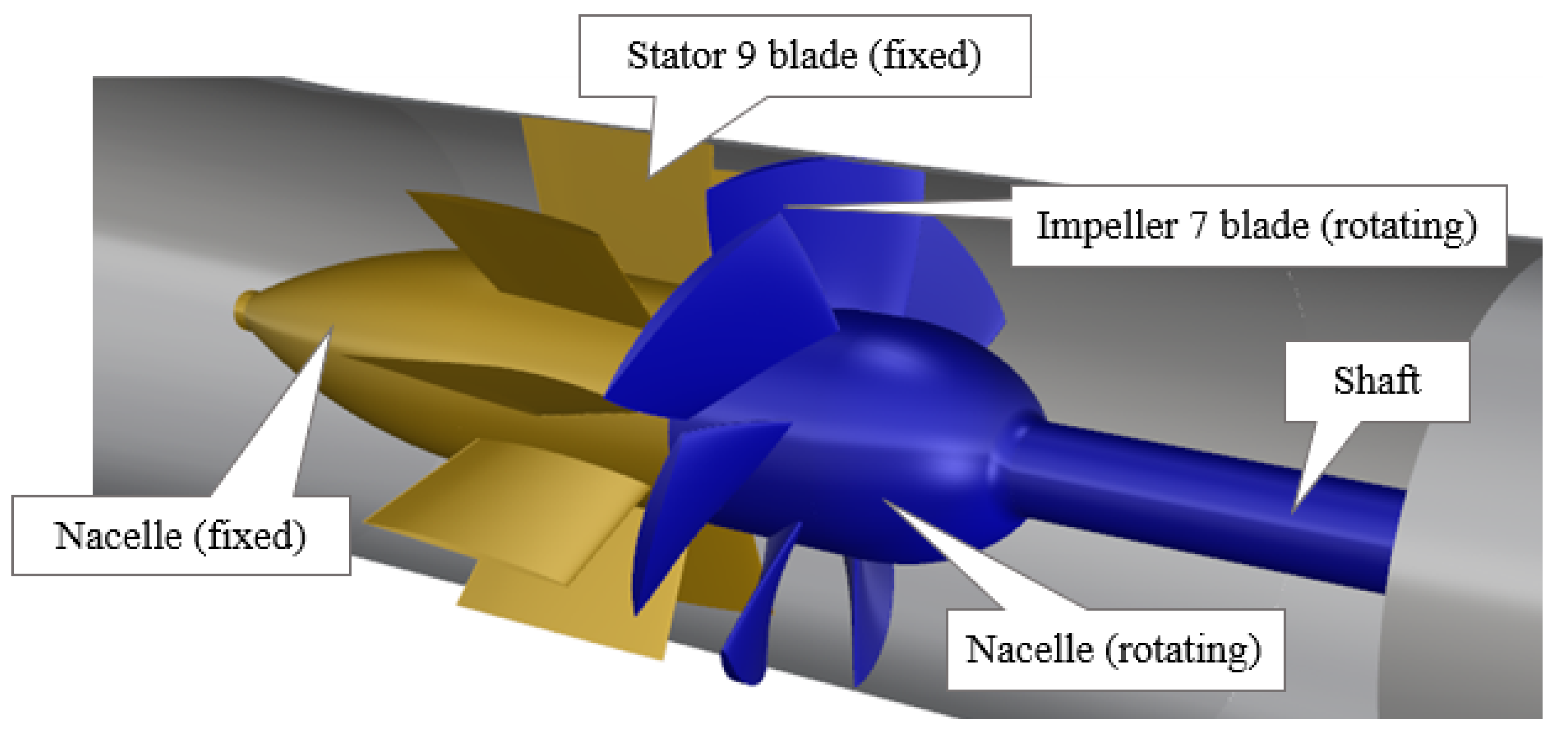
Figure 2 shows the geometry of the pump of the DLCT. The impeller has a 0.1% gap between the blade tip and the tunnel wall, and it rotates counterclockwise when looking upstream. The stator is fixed by attaching the blade end to the tunnel wall. Table 1 shows the particulars of the impeller and stator. In the case of the stator, it has a large mean pitch ratio because the stator refines the tangential flow caused by the impeller, and the impeller has a relatively small mean pitch ratio. The nacelle diameter ratio is 0.45, and the nacelle nose is a rotating body that has a streamlined shape of the third order. The nacelle also has a parallel-sided body with the same diameter at the location of the impeller and stator, and it is 9.46 m long. The tail of the nacelle is also a streamlined shape of the third order. The design RPM is 83 at the maximum flow speed VT = 15 m/s in the test section.
3. Numerical Methods
For the 3-dimensional steady-state incompressible turbulent flow, the governing equations are continuity and momentum equations (RANS equations), as shown in Equations (1) and (2), respectively.
where, is the velocity component in direction, is the water density, is the kinematic viscosity, p is the static pressure, and is the gravitational acceleration in i-direction. The is the Reynolds stress and is given by Equation (3) using the isotropic eddy viscosity model of the Boussinesq hypothesis.
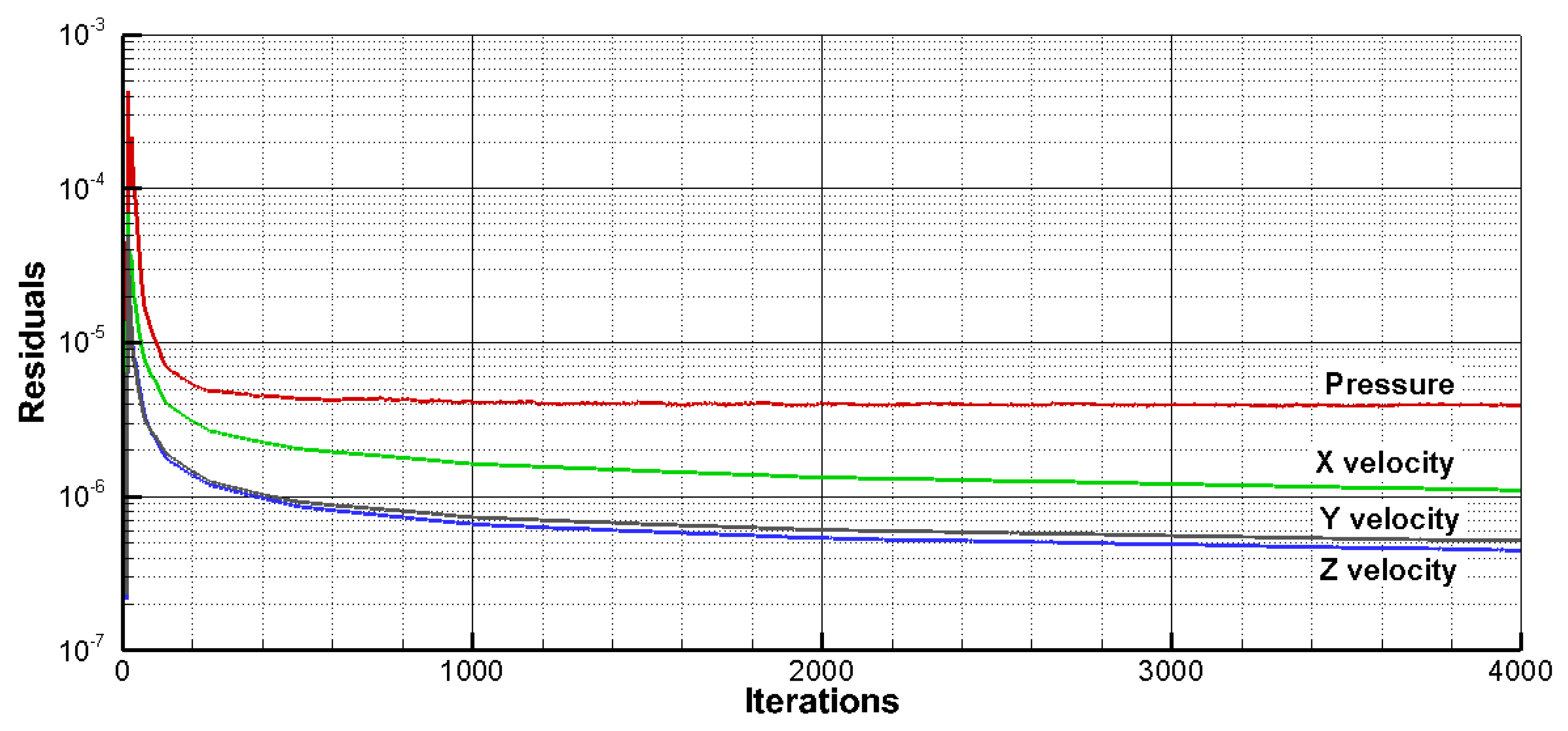
where is the turbulent kinetic energy, is the Kronecker delta. The is the turbulent eddy viscosity, and the realizable k-ϵ turbulence model is used to calculate the . In the standard k-ϵ model, is generally 0.09, but in the realizable k-ϵ model, it is given as a function of shear and vorticity [12]. The realizable k-ϵ is used often in calculating the turbulent flow of the tunnel and used widely in the hull form calculation; it is well known to give good results for hull resistance and vortex flows on a propeller plan [13,14,15]. It has also been shown that the realizable k-ϵ model gives good results for the performance of marine propellers [16]. Therefore, the realizable k-ϵ turbulence model can be considered to be suitable for this study on the impeller of the axial pump in terms of vortex flow and the force of a rotating body, such as that of a propeller. The standard wall function is used. In this case, a normalized distance of a first grid point from the wall () must be located in the log layer. Usually, the logarithmic law of the wall, i.e., log law, is satisfied, in which is over about 60, and the range of satisfying the log law increases according to the Reynolds number increment. Thus, can be determined appropriately considering the Reynolds number. The Reynolds number of the impeller at 0.7R is about based on the relative velocity, considering the impeller rotation, and the Reynolds number of the stator is about based on the tunnel flow speed. Thus, considering the Reynolds number, is maintained at about 200 following reference [16]. Through a process of discretization based on the finite volume method, the algebraic equations are solved. A commercial CFD code, Fluent (V17), was used for the computations. The convection and diffusion terms of momentum equation given by Equation (2) were discretized by QUICK and the second-order central-difference scheme, respectively. The SIMPLEC algorithm was used for the velocity–pressure coupling, and the Euler–Euler approach was adopted to simulate the flow. An MRF (moving reference frame) scheme was adopted for the impeller rotation [12]. The calculations were regarded to be converged, as the residuals of the velocity and the pressure were lower than . The residuals were defined as the differences between a previous result and the subsequent result in the calculation step.
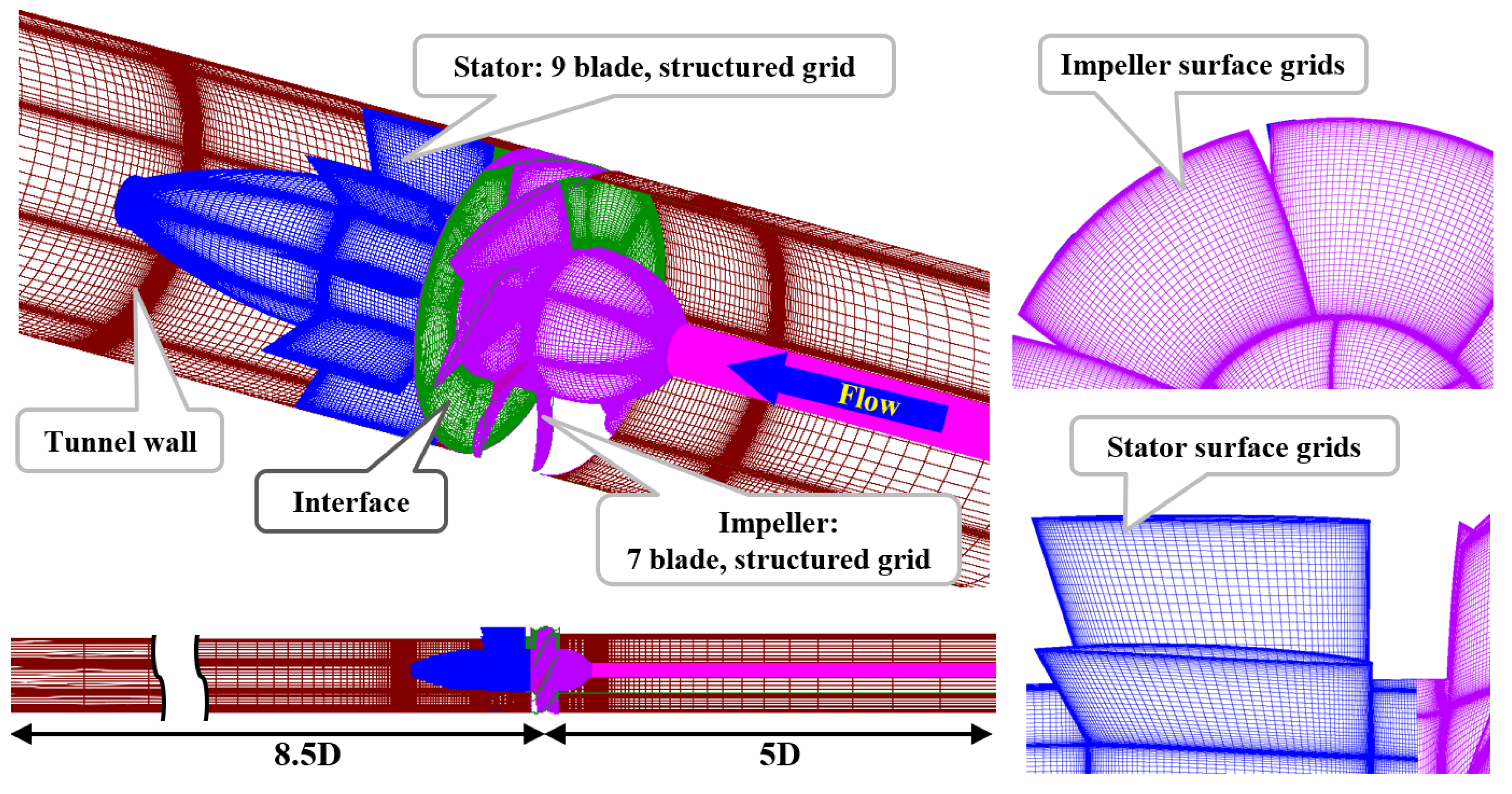
The coordinate system consisted of an origin at the center of the impeller, and the main flow direction towards positive x and the vertical direction towards positive z. A three-dimensional structured grid system was used in the entire domain, as shown in Figure 3. The boundaries of that are defined as follows: the inlet boundaries are located at 5D upstream from the impeller center with the velocity inlet condition; the outlet boundary is located at 8.5D downstream with the pressure outlet condition. Since the impeller and the stator are operated in the circular tunnel, the external boundary is the tunnel wall with the no-slip condition.
A multi-block grid for using the MRF scheme was generated and then the grids were divided into two blocks: a fixed block and a rotating block. The number of grids applied in the numerical analysis was approximately 11 million: 5 million in the rotating block for the impeller and 6 million in the fixed block including the stator. The impeller surface grids were finely distributed near the propeller tip. The spatial grids around the impeller were composed of seven grid blocks, and each block was made of spatial grids between the pressure side of the reference blade and the suction side of the next blade. The spatial grids around the stator were composed of nine grid blocks; thus, the grid points between the impeller and the stator did not match. The patched boundaries faced between them were treated as interfaces. Additionally, since there was a gap between the tunnel wall and the impeller tip, it was treated as an interface as well, and the number of grid layers in the gap was six. Table 2 shows the thrust and the torque coefficient of the pump, which followed Equation (6), according to the number of grids. The number of grids for the grid dependency was increased by times. It can be seen that the thrust and the torque coefficients almost converge after case 2. Thus, the subsequent calculations for the pump were conducted using the grid system of case 2.
4. Pump Performance
Numerical analyses were carried out for an axial flow pump operating in a cylindrical tunnel, and the performance of pump was investigated. The flow rate in the pump was determined by the speed in the test section. The pump flow rate was obtained from the maximum speed, 15 m/s, and the general speed, 7.5 m/s, in the test section. The pump flow speeds corresponded to the speed in the test section. The rotating speed changed based on varying the capacity coefficient () or the advanced ratio (J). Table 3 represents the calculation conditions.
Pump performances are generally characterized in terms of head, and non-dimensional variables related to pump performance are defined as Equation (4).
where is the capacity coefficient, is the head coefficient, is the power coefficient, is the efficiency of the pump, is the flow rate (), is the revolution per second (), D is the diameter of pump, g is gravity, H is the pump head, is the angular velocity, and Q is the torque of the impeller. The head (H) increase in the axial flow pump is obtained by calculating the average pressure (P) and average velocity (V) as in Equation (5). Here, is a kinetic energy correction factor to consider as a boundary layer and is a local velocity. The positions of the inlet and the outlet to calculate the head are x/D = −1 upstream of the impeller, and x/D = 2 downstream of the stator, respectively.
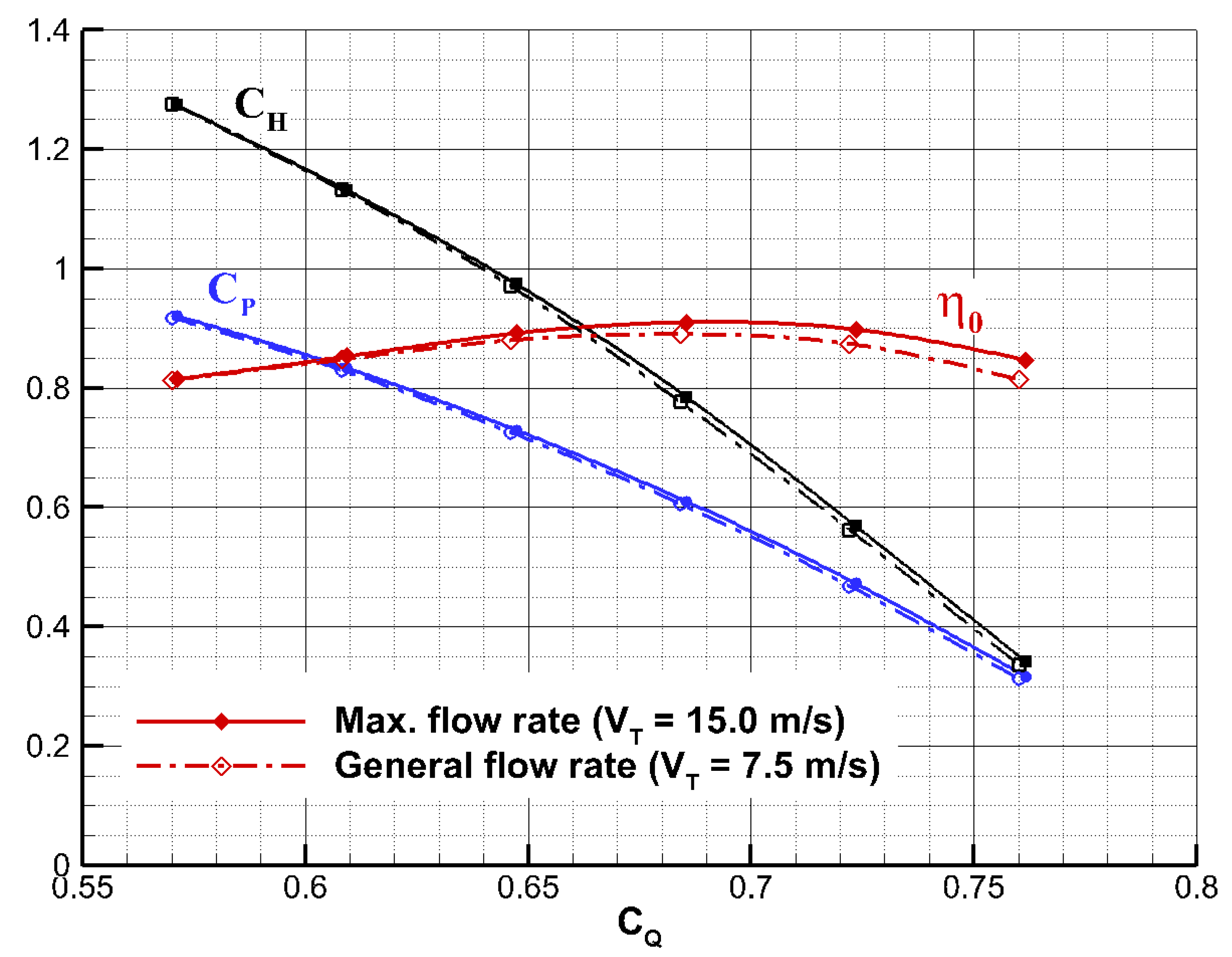
Figure 4 shows the representative residual history for the calculation of at the maximum test section speed. The residuals decease rapidly in the beginning of the calculation and then it becomes smaller than the residual criterion of . Thus, the solution can be regarded as being converged. Figure 5 shows the performance curves of the pump. and are decreased as increases. The change in efficiency is relatively small, and the maximum efficiency is about 0.91, near . Because the diameter of the tunnel is constant, the flow rate is the same, and the decreases as the rotating speed increases. Accordingly, the angle of attack of the impeller blade increases so that the and increase. The thrust and the torque in the maximum speed are larger than those in the general speed. Moreover, the efficiency of the maximum speed is larger than that of the general speed because the increase in thrust is greater than the increase in torque. As the Reynolds number increases, the friction loss reduction due to the relatively thin boundary layer thickness appears as this scale effect. There is no significant difference in efficiency according to the flow coefficient; therefore, it would be desirable to set a flow coefficient between 0.65 and 0.75, which is near the maximum efficiency, to the design point.
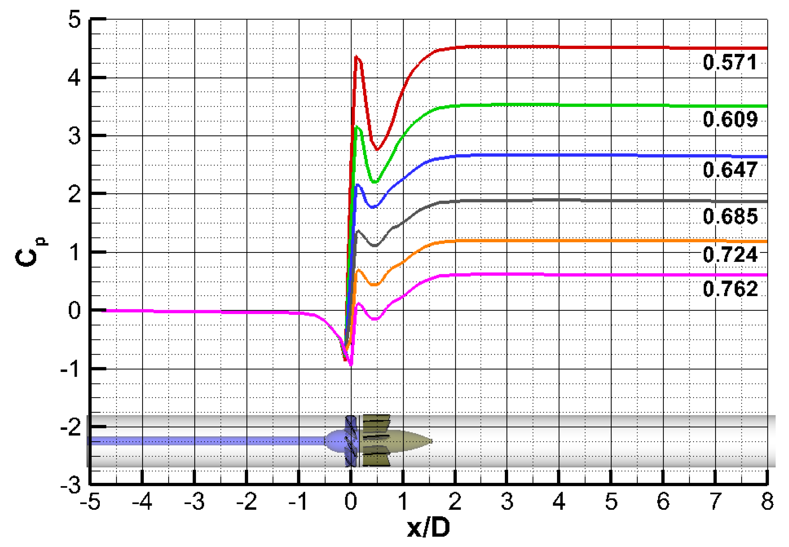
Figure 6 shows the pressure distribution on the cylindrical tunnel wall, and the pressure is normalized by dynamic pressure (). There is almost no difference in pressure in front of the impeller, but the pressure jump appears after passing through the impeller. The load of the impeller increases as the rotating speed of the impeller increases, so that the decreases, resulting in a larger pressure recover in the downstream. Because the impeller operates in the cylindrical tunnel and the flow rate is constant, there is no flow acceleration in the downstream; there is only the effect of increasing the pressure. The pressure drop by the friction loss of the tunnel wall in upstream and downstream is small but can be observed.
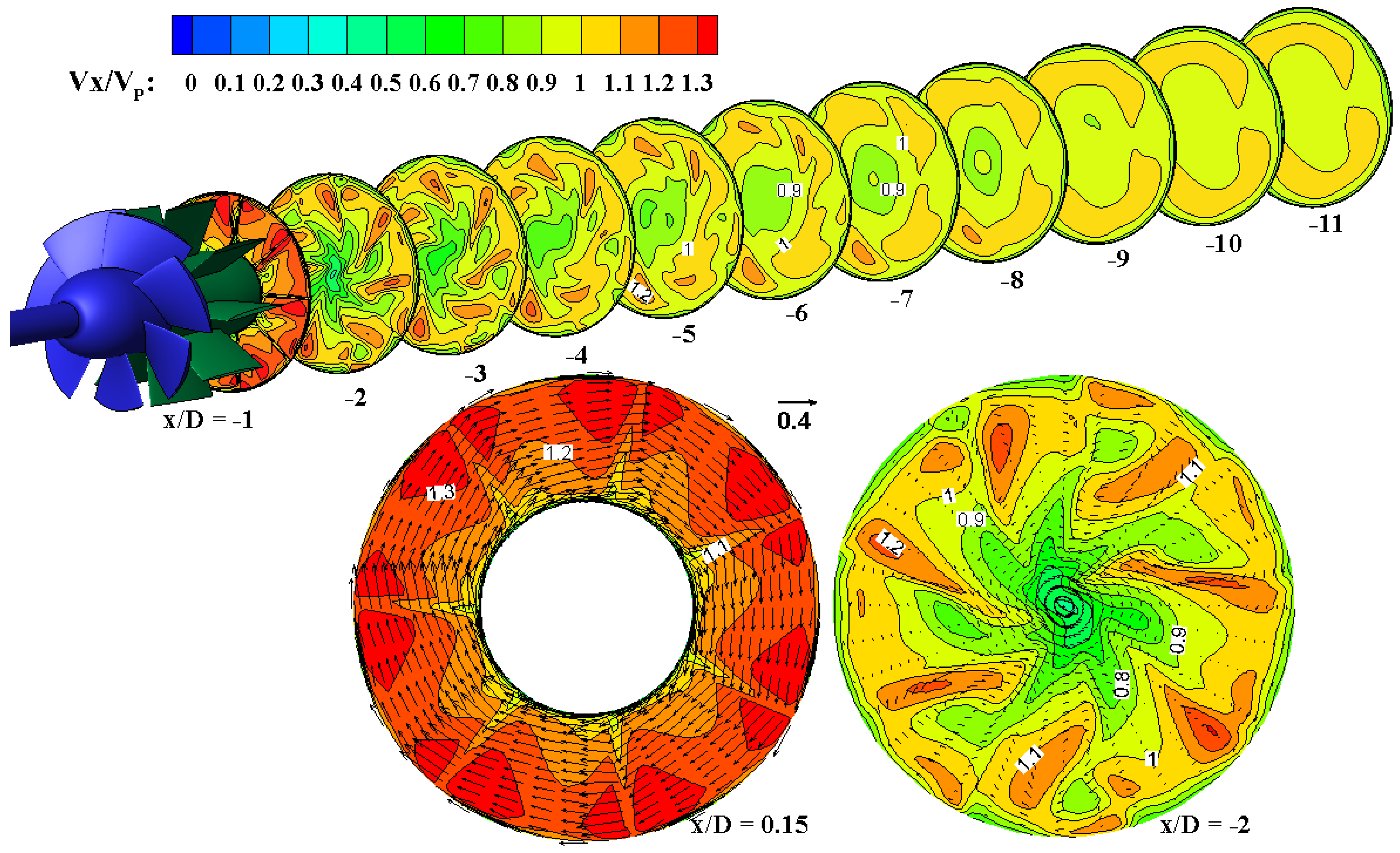
On the other hand, the stator is attached to the tunnel wall and serves as a structural part, and it also refines the rotational flow of the impeller wake. Figure 7 shows the distribution of the axial velocity distributions along the streamwise direction and the velocity distribution with the cross vector at the x/D = 0.15 section right behind the impeller and the x/D = 2 section after the stator. The axial acceleration and rotational flow in the outer radius are strong. This is due to the impeller and the reduction in the flow path area by the nacelle. The rotational flow appears to be about 30% of the inflow speed. After the flow past the stator, some traces of acceleration remain, but it was found that the rotational flow almost disappears. This flow acceleration decreases toward the downstream, and the flow mixes so that it becomes relatively uniform. The stator can be considered to play a sufficient role, and this can be confirmed from the open water performance when the impeller is regarded as a propeller of ship in terms of force. Especially, it is difficult to distinguish the roles played by each part with only the head coefficient given by Equation (5), so it is necessary to examine the force appearing in each part. The thrust and the torque of the parts are normalized as Equation (6).
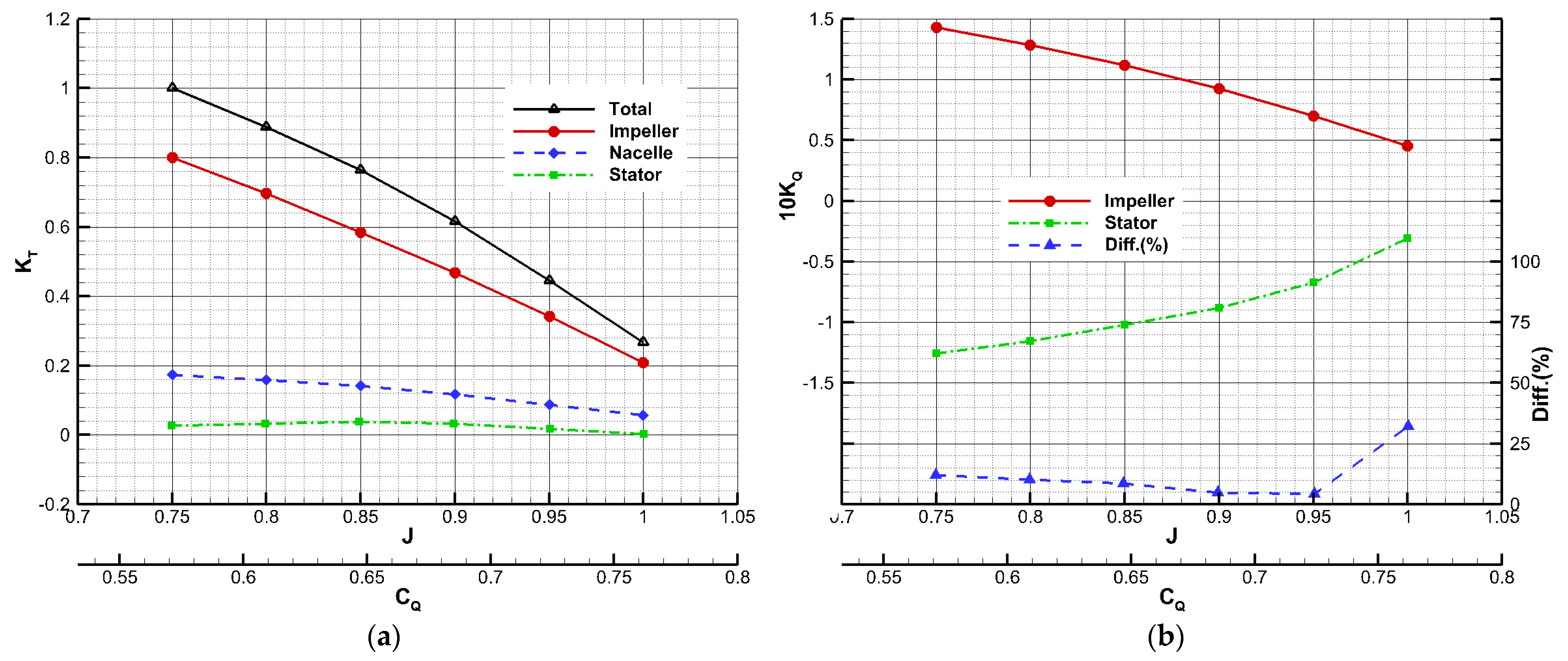
where J is an advanced ratio as , is a thrust coefficient as , and is a torque coefficient as . Figure 8 shows the thrust and the torque coefficient for each part. The thrust of the impeller is dominant, but the stator and nacelle also generate thrust. The stator with a very large pitch has a large angle of attack due to the rotational flow by the impeller, and it thus generates the thrust. In the case of the nacelle, as shown in Figure 6, the thrust is generated due to the pressure recovery in the tail, which is relatively as large as about 20% of the total thrust. From this, it is confirmed that the impeller, nacelle, and stator also play a role in increasing the head. Figure 8b shows the torques of the impeller and the stator. Here, the torque of the impeller is the input power for rotating the impeller, and since the torque of the stator does not actually rotate, it can be regarded as the flow work that occurs when the rotational flow by the impeller flows into the stator. Therefore, the impeller and the stator torque have different signs, and the rotational flow is reduced by the torque of the stator that turns the flow in the opposite direction. The difference in the magnitude of the torques of the two parts is about 10% in the low advanced ratio, and the difference decreases as the rotational speed decreases, i.e., the advanced ratio increases. It can be inferred that the flow refinement effect of the stator appears well as the rotating speed decreases.
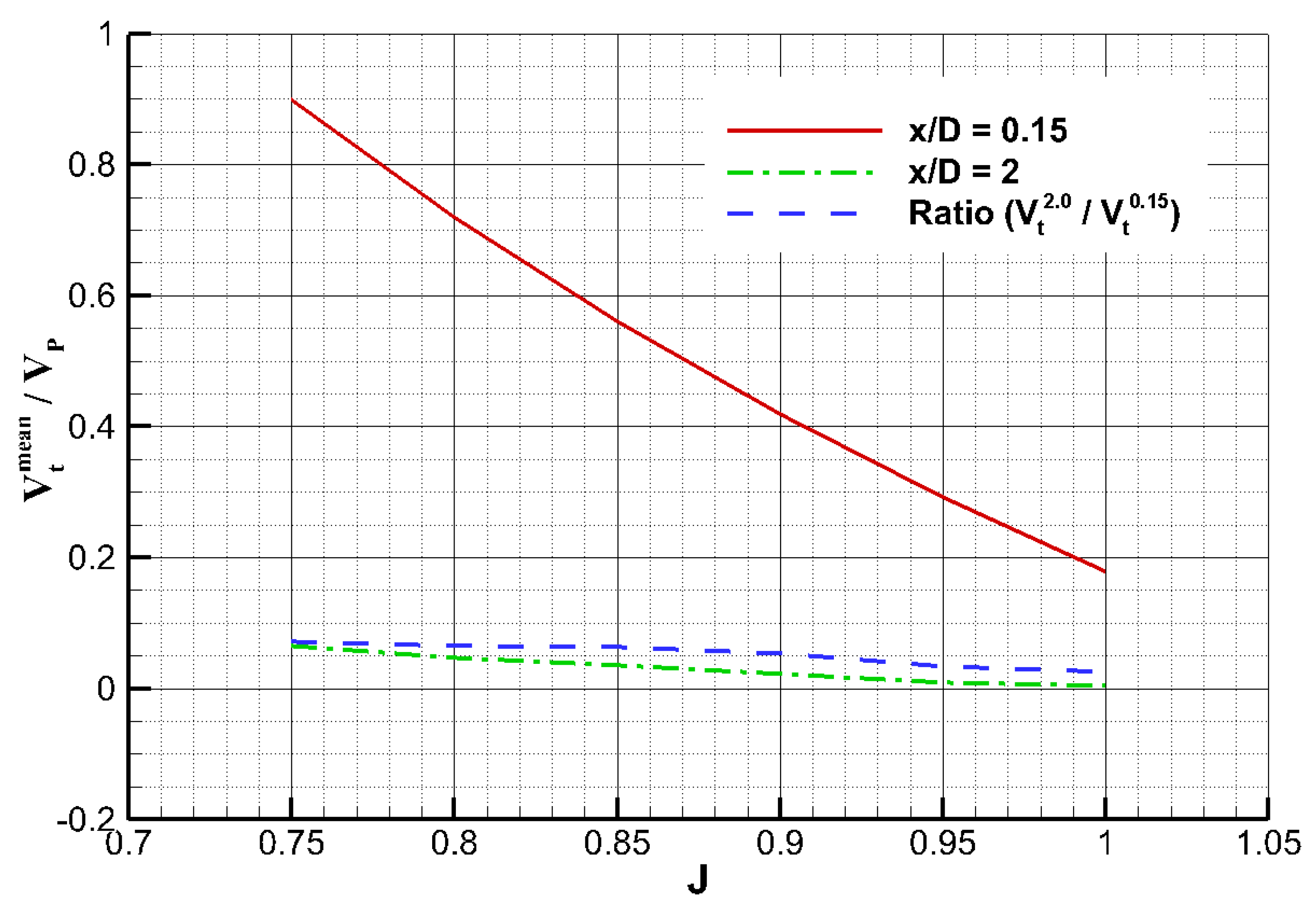
To confirm this, Figure 9 shows the averaged tangential velocity () in the wake after the nacelle. The larger the load, the greater the tangential flow caused by the impeller, and the tangential velocity decreases as the advanced ratio decreases. At x/D = 2, it appears that the tangential flow is very reduced, and it decreases to about 7% of the tangential velocity induced by the impeller, and decreases further as the advanced ratio increases. In particular, the cases of J = 0.95 and 1.00 are 3.4% and 2.6%, respectively, and on overall average, it is about 5.2%. Since the tangential flow is reduced by the stator more than 95% of that by the impeller, it is confirmed that the stator plays a significant role.
As above, the performance of the axial flow pump was investigated. In order to investigate the actual operating performance of the DLCT, the head identity was used so that the operating point could be obtained by matching the head loss of the large cavitation tunnel with the head gain of the axial flow pump. To obtain the head loss of the DLCT, a numerical analysis was performed on the entire tunnel without the pump.
5. Target Head of DLCT
When applying the axial flow pump directly to the large cavitation tunnel, it is necessary to introduce a numerical technique that directly rotates the impeller (sliding mesh) due to the asymmetry of the flow. However, since it is necessary to perform an unsteady analysis and since it takes a lot of time to calculate, direct analysis is difficult. Therefore, it is efficient to perform steady-state analyses separately for the large cavitation tunnel and for the axial flow pump so that it can provide information on the operating point of the tunnel from the head identity. For this, the numerical analyses were performed on the DLCT, except for the impeller and the stator. The numerical methods were applied in the same way, except for the rotating effect, as mentioned above. The flow speed conditions in the test section () were 5 at 2.5 m/s intervals between 5 m/s and 15 m/s.
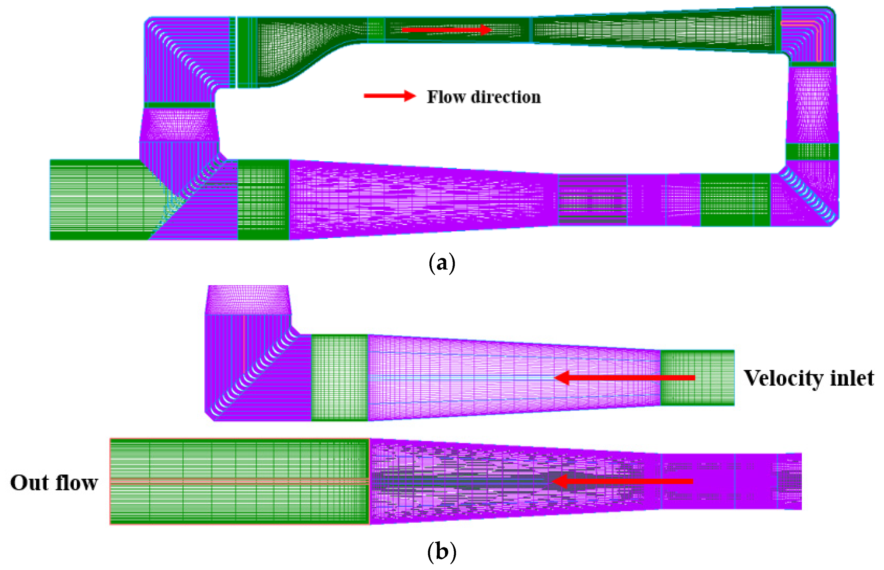
The coordinate system consisted of the origin at the center of the tunnel entrance top and the main flow direction towards positive x and the vertical direction towards positive z. A three-dimensional structured grid system was used except for the second corner, as shown in Figure 10. In the case of the second corner, since the generation of the structured grid was difficult due to the complicated shape—such as the guide vanes, shaft, housing, and the flow splitter—a structured grid was used in the vicinity of the vanes for boundary layer calculation, and in the other, an unstructured grid was used. The velocity inlet condition was given at the impeller position of the lower leg diffuser without nacelle and impeller, and a pressure outlet condition was applied at the end of domain that was added by a certain length from the exit of the lower leg diffuser with the nacelle, as shown in Figure 10b. Although the inlet and outlet grid systems overlapped each other, they were created in different blocks, so there were no problems numerically. The total number of grids was about 22 million.
On the other hand, the flow straightener was modeled to the 0.1 m square tube with 0.25 m length of 6000 EA, and a structured grid system was used. Patched faces between the flow straightener block and the fourth corner block were treated as an interface boundary condition. A porous model was used for the honeycomb. The porous model can achieve the effect of the honeycomb without directly modeling the honeycomb by substituting the momentum sources for the force acting on the honeycomb at that position in the flow field. The body force is the momentum per unit volume, and the force acting on an object must be properly estimated in advance and replaced with the body force. In the case of honeycomb, since the force of the vertical and horizontal direction can be expected to be quite large due to blocking by the wall of the honeycomb, a flow refinement effect appears, and from this, the momentum of vertical and horizontal direction can be determined such that the values are large enough. In the main flow direction, the drag force caused by the friction of the honeycomb varies depending on the flow speed, so the head loss could be estimated from the formula according to the Reynolds number of the honeycomb. A head loss estimation of honeycomb follows reference [17]. The details of the numerical methods can be found in reference [18].
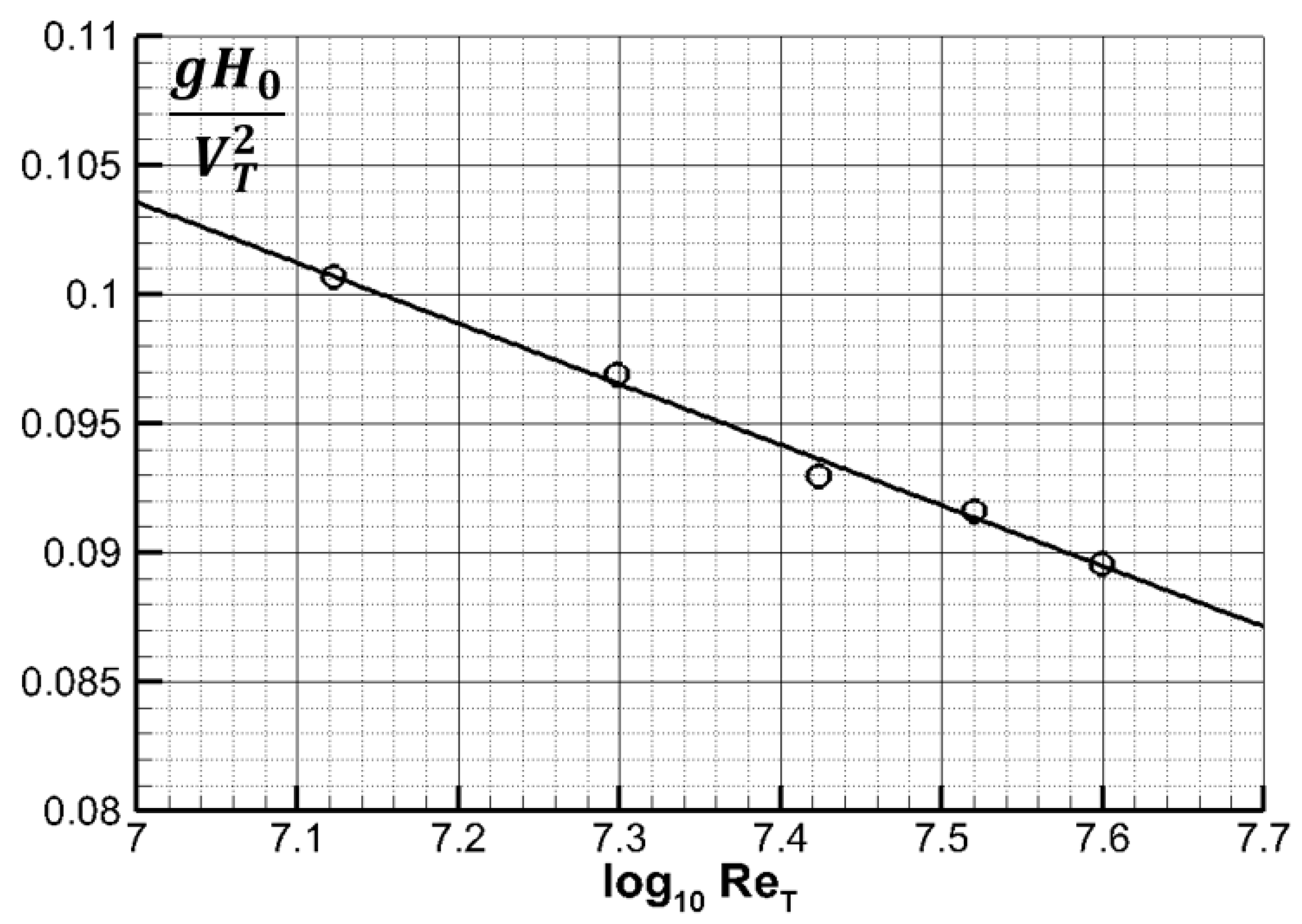
The purpose of this study was to estimate the performance of the axial flow pump and to provide information on the operating point of the DLCT, so only the head loss of the DLCT is discussed, and the other performances, such as flow quality, are excluded. The head loss of the DLCT from the numerical analysis result was obtained from Equation (2) using the pressures and the velocities in the inlet and the outlet boundaries. Figure 11 shows the non-dimensional head loss of the DLCT estimated from the numerical analysis results. Here, the horizontal axis is the log scale for Reynolds numbers, which is normalized by the hydraulic diameter of cross-section of the test section (). As the Reynolds number increases, i.e., the flow speed of the test section increases, the head loss coefficient decreases almost linearly. Since most of the loss is due to friction, it decreases logarithmically with the Reynolds number.
6. Estimation of DLCT Performance
As described above, the head loss of the DLCT without the pump was estimated. From this, the operating point of the tunnel was estimated. To estimate the rotating speed when driving the impeller in the large cavitation tunnel, a specific speed () was first defined as in Equation (7).
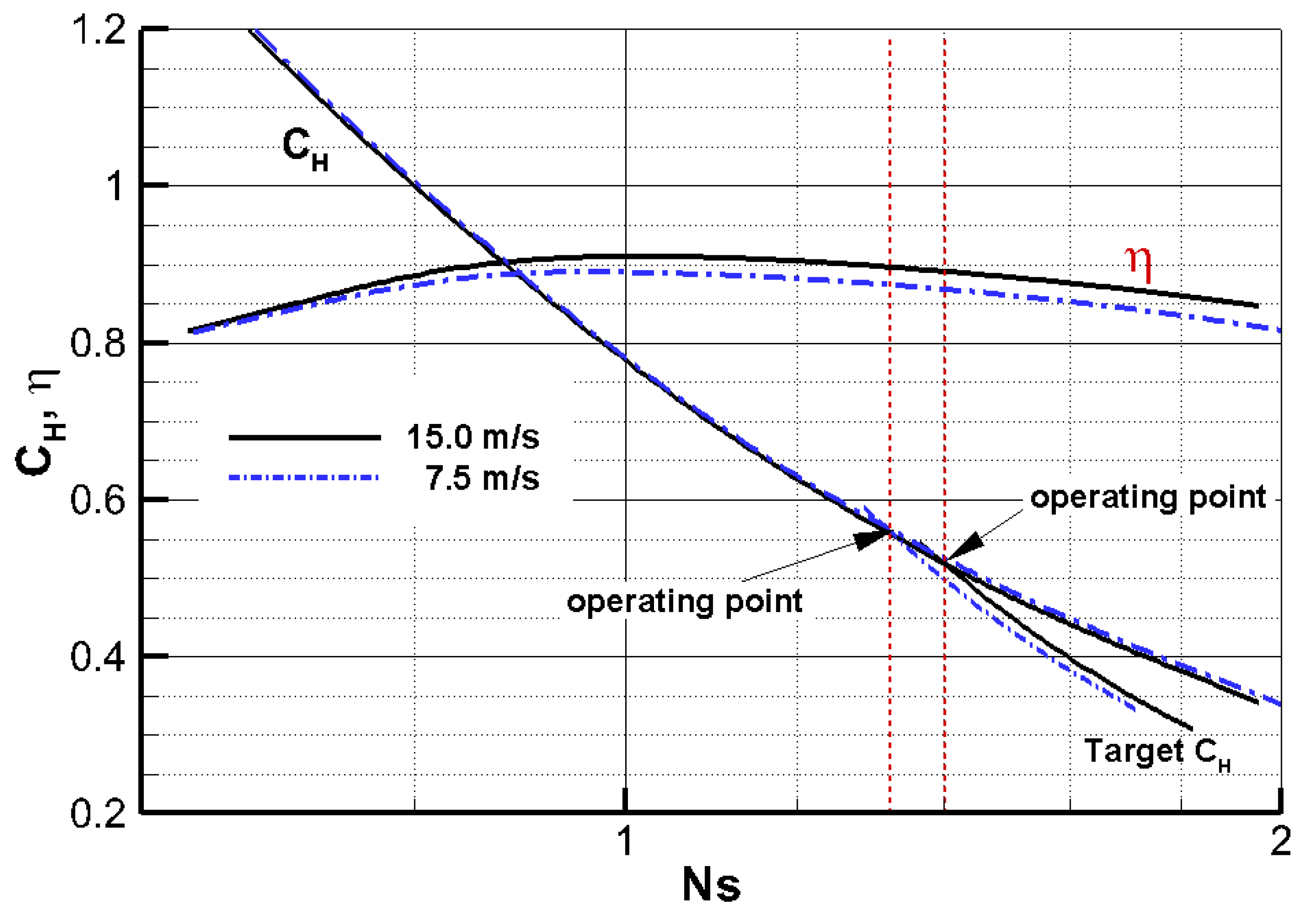
In order to obtain the specific speed from the head loss of the DLCT, the numerical analysis result was used. The head loss of the tunnel () and the flow rate () corresponding to the certain test section speed were fixed, and then the specific speeds for that could be obtained using Equation (7) by changing the impeller rotating speed (). The specific speed of the pump could be obtained using the head gain of the pump (). These are shown together in the specific speed–head coefficient graph, finding the point where the two curves meet as shown in Figure 12.
Consequently, the specific speed values can be read by drawing a straight line perpendicular to the horizontal axis from the point where the two curves meet, and that point is the operating point in the flow rate. So, the rotating speed of the impeller can be calculated using Equation (7). And then the efficiency and the power coefficient can be obtained from the Figure 5. Figure 12 shows the specific speed–head coefficient curves for the axial flow pump and large cavitation tunnels for the two test section speeds. For each speed, the point where the pump head meets the tunnel head can be found, and the information is shown in Table 4.
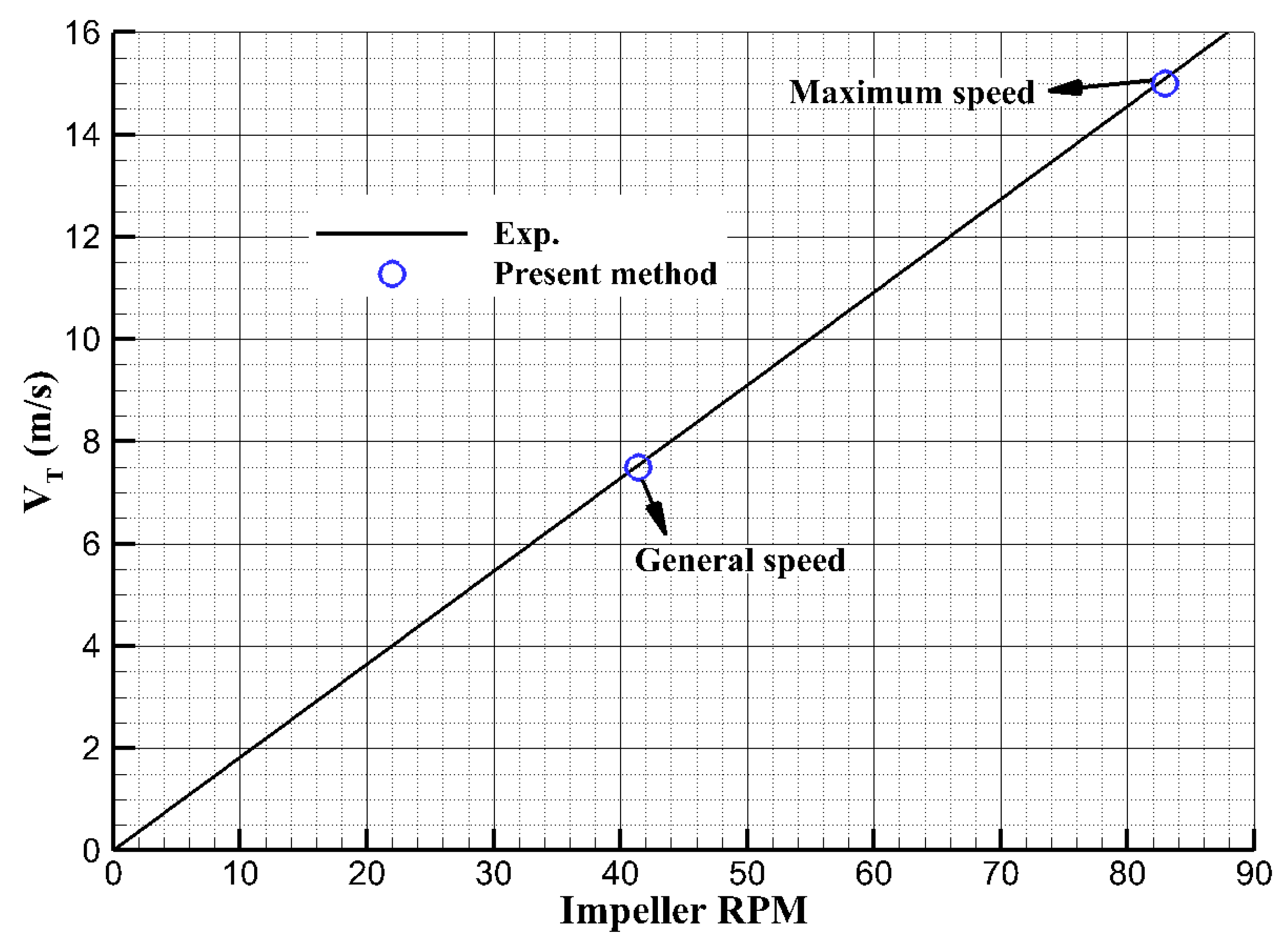
At the maximum speed, the target head coefficient is about 0.517 and the rotation speed in the operating point is 82.97 RPM. This is estimated to be approximately the same as the design rotating speed as shown in Table 1. The general flow speed is half of the maximum flow speed, and the rotating speed of the impeller can be found as 41.39 RPM from Figure 12, which is about half of the rotating speed in maximum flow speed.
It can be inferred that the flow speed of the test section according to the impeller rotating speed can appear to be almost linear. In the case of efficiency, it is about 0.89 at the maximum flow speed and about 0.87 at the general flow speed. Although it is less than the maximum efficiency of the pump (0.91), the efficiency is considerable level. Figure 13 shows the flow speed in the test section of the experiments and the present numerical results. The experiments were carried out at the DLCT of the Daewoo Shipbuilding and Marine Engineering Siheung R&D center. The results obtained in this study are in good agreement with the experimental results.
7. Conclusions
In this study, a numerical analysis was used to investigate the performance of the axial flow pump for a large cavitation tunnel. Numerical analyses for an axial flow pump composed of an impeller, a stator, and a nacelle located in a cylindrical tunnel were performed by varying the rotating speed of the impeller under the conditions of the maximum and the general flow speeds in the test section. From this, the flow characteristics, force, and torque performance of the axial flow pump were investigated, and the rotating speeds of the impeller satisfying the test section speed performances required in the large cavitation tunnel were estimated.
The head gain was confirmed to be caused by the pressure jump in the downstream of the pump, and thrust was generated not only in the impeller but also in the stator and nacelle, contributing to the increment in the head gain. The stator was intended to refine the rotational flow due to the rotation of the impeller, and a refinement effect of more than 95% on average was confirmed.
In order to obtain the operating point using the head identity, numerical analysis was carried out according to the flow speed in the test section for the large cavitation tunnel without the pump, and the total head loss of the tunnel was estimated. As the Reynolds number of the test section increased, the head coefficient decreased logarithmically with the Reynolds number. Using the head loss of the large cavitation tunnel, the operating point was obtained from the specific speed–head coefficient curve by matching the head gain of the pump. The rotating speed of the impeller at the obtained operating point was almost the same as that of the experiments, and an axial flow pump with excellent performance was confirmed to have been designed.
Author Contributions
Conceptualization, J.-K.C., H.-T.K., C.-S.L. and S.-J.L.; methodology, J.-K.C., H.-T.K. and C.-S.L.; software, J.-K.C.; validation, J.-K.C., H.-T.K. and C.-S.L.; formal analysis, J.-K.C. and H.-T.K.; investigation, J.-K.C.; resources, J.-K.C., H.-T.K. and C.-S.L.; data curation, J.-K.C., H.-T.K., C.-S.L. and S.-J.L.; writing—original draft preparation, J.-K.C.; writing—review and editing, J.-K.C., H.-T.K., C.-S.L. and S.-J.L.; visualization, J.-K.C.; supervision, J.-K.C.; project administration, C.-S.L.; funding acquisition, C.-S.L. and S.-J.L. All authors have read and agreed to the published version of the manuscript.
Funding
This research was funded by Daewoo Shipbuilding and Marine Engineering Co. Ltd.
Institutional Review Board Statement
Not applicable.
Informed Consent Statement
Not applicable.
Data Availability Statement
The data presented in this study are available in this article (Tables and Figures).
Conflicts of Interest
The authors declare no conflict of interest.
References
- Wilson, M.B.; Etter, R.J. Hydrodynamic and hydro-acoustic characteristics of the new David Taylor model basin large cavita-tion channel. In Proceedings of the 2nd International Symposium on Propellers and Cavitation, Hangzhou, China, 1–4 September 1992; pp. 305–311. [Google Scholar]
- Ahn, J.-W.; Kim, G.-D.; Kim, K.-S.; Park, Y.-H. Performance Trial-Test of the Full-Scale Driving Pump for the Large Cavitation Tunnel (LCT). J. Soc. Nav. Arch. Korea 2015, 52, 428–434. [Google Scholar] [CrossRef]
- Wetzel, J.M.; Arndt, R.E.A. Hydrodynamic Design Considerations for Hydroacoustic Facilities: Part I—Flow Quality. J. Fluids Eng. 1994, 116, 324–331. [Google Scholar] [CrossRef]
- Kyparissis, S.D.; Margaris, D.P. Experimental Investigation and Passive Flow Control of a Cavitating Centrifugal Pump. Int. J. Rotating Mach. 2012, 2012, 1–8. [Google Scholar] [CrossRef] [Green Version]
- Zhang, S.; Zhang, R.; Zhang, S.; Yang, J. Effect of impeller inlet geometry on cavitation performance of centrifugal pumps based on radial basis function. Int. J. Rotat. Mach. 2016, 2016, 6048263. [Google Scholar] [CrossRef] [Green Version]
- Hatano, S.; Kang, D.; Kagawa, S.; Nohmi, M.; Yokota, K. Study of Cavitation Instabilities in Double-Suction Centrifugal Pump. Int. J. Fluid Mach. Syst. 2014, 7, 94–100. [Google Scholar] [CrossRef] [Green Version]
- Jiang, Z.; Li, H.; Shi, G.; Liu, X. Flow Characteristics and Energy Loss within the Static Impeller of Multiphase Pump. Processes 2021, 9, 1025. [Google Scholar] [CrossRef]
- Hosono, K.; Kajie, Y.; Saito, S.; Miyagawa, K. Study on cavitation influence for pump head in an axial flow pump. J. Phys. Conf. Ser. 2015, 656, 012062. [Google Scholar] [CrossRef] [Green Version]
- Ahn, J.-W.; Kim, G.-D.; Kim, K.-S.; Lee, J.-T.; Seol, H.-S. Development of the Driving Pump for the Low Noise Large Cavitation Tunnel. J. Soc. Nav. Arch. Korea 2008, 45, 370–378. [Google Scholar] [CrossRef] [Green Version]
- Li, W.-G. NPSHr Optimization of Axial-Flow Pumps. J. Fluids Eng. 2008, 130, 074504. [Google Scholar] [CrossRef]
- Watanabe, T.; Sato, H.; Henmi, Y.; Horiguchi, H.; Kawata, Y.; Tsujimoto, Y. Rotating Choke and Choked Surge in an Axial Pump Impeller. Int. J. Fluid Mach. Syst. 2009, 2, 232–238. [Google Scholar] [CrossRef] [Green Version]
- ANSYS. Fluent User’s Guide; ANSYS: Canonsburg, PA, USA, 2018. [Google Scholar]
- Kim, J.; Park, I.R.; Kim, K.S.; Van, S.H. RANS Simulations for KRISO Container Ship and VLCC Tanker. J. Soc. Nav. Archit. Korea 2005, 42, 593–600. [Google Scholar]
- Kim, B.-N.; Kim, W.-J.; Kim, K.-S.; Park, I.-R. The Comparison of Flow Simulation Results around a KLNG Model Ship. J. Soc. Nav. Arch. Korea 2009, 46, 219–231. [Google Scholar] [CrossRef] [Green Version]
- Lee, C.-M.; Seo, J.-H.; Yu, J.-W.; Choi, J.-E.; Lee, I. Comparative study of prediction methods of power increase and propulsive performances in regular head short waves of KVLCC2 using CFD. Int. J. Nav. Arch. Ocean. Eng. 2019, 11, 883–898. [Google Scholar] [CrossRef]
- Choi, J.-K.; Kim, H.-T. An investigation on the effect of the wall treatments in RANS simulations of model and full-scale marine propeller flows. Int. J. Nav. Arch. Ocean. Eng. 2020, 12, 967–987. [Google Scholar] [CrossRef]
- Barlow, J.B.; Rae, W.H.; Pope, A. Low-Speed Wind Tunnel Testing, 3rd ed.; John Willy & Sons: New York, NY, USA, 1984; pp. 90–91. [Google Scholar]
- Choi, J.K.; Kim, H.T.; Lee, C.S.; Lee, S.J.; Yoon, H. Numerical Study on the Flow of Test section and Diffuser of Large Cavitation Tunnel. In Proceedings of the 11th International Symposium on Cavitation, Daejeon, Korea, 10–13 May 2021; pp. 266–270. [Google Scholar]
Figure 1.
Geometry of DSME Large Cavitation Tunnel.

Figure 2.
Impeller and stator geometry.

Figure 3.
Grid system of impeller and stator.

Figure 4.
Residuals history for at the maximum test section speed.

Figure 5.
Performance curves of the axial flow pump.

Figure 6.
Pressure distributions on the tunnel wall by CQ.

Figure 7.
Velocity distribution behind impeller (x/D = 0.15) and stator (x/D = 2) at for .

Figure 8.
Thrust and torque performance curves of the pump parts for . (a) Thrust performance of the pump parts. (b) Torque performance of the pump parts.
Figure 8.
Thrust and torque performance curves of the pump parts for . (a) Thrust performance of the pump parts. (b) Torque performance of the pump parts.

Figure 9.
Tangential mean velocities according to advanced ratio for = 15 m/s.

Figure 10.
Grids system and boundary conditions of DSME large cavitation tunnel. (a) Overall domain. (b) Boundary conditions.
Figure 10.
Grids system and boundary conditions of DSME large cavitation tunnel. (a) Overall domain. (b) Boundary conditions.

Figure 11.
Head loss of the DLCT according to Reynolds numbers from the numerical results.

Figure 12.
Specific speed–head coefficient curves of the axial flow pump.

Figure 13.
Test section speed according to the impeller RPM.


Table 1.
Particulars of the axial flow pump.
| Particulars | Impeller | Stator |
|---|---|---|
| Diameter (m) | 4.6 (cutting edge 5 mm) | 4.6 |
| (P/D) mean | 1.428 | 37.517 |
| Ae/A0 | 0.992 | 1.513 |
| Nacelle Dia. ratio | 0.450 | 0.450 |
| No. of blades | 7 | 9 |
| Section | NACA 66 | NACA 66 |
| Shaft dia. (m) | 0.8 | - |
| Design RPM | 83 at test section speed 15 m/s | - |
| Re at 0.7R | 3.5 × 10⁷ | 1.0 × 10⁷ |
| Rotating | Counterclockwise | Fixed |
Table 2.
Grid dependency test and the results at J = 0.85.
| Case | No. of Grid | KT | 10KQ | Selection | |||
|---|---|---|---|---|---|---|---|
| Rotating Block (Impeller) | Stationary Block | Total | |||||
| Stator | Tunnel | ||||||
| 1 | 3.5 M | 2.0 M | 3.0 M | 8.5 M | 0.7656 | 1.1210 | |
| 2 | 5.0 M | 3.0 M | 3.0 M | 11.0 M | 0.7649 | 1.1178 | O |
| 3 | 7.0 M | 4.2 M | 3.0 M | 14.2 M | 0.7650 | 1.1178 | |
Table 3.
Calculation conditions.
| Particulars | Maximum | General |
|---|---|---|
| Flow speed in test section () | 15 m/s | 7.5 m/s |
| Pump flow speed () | 6.128 m/s | 3.064 m/s |
| Flow rate () | 98.76 m3/s | 49.38 m3/s |
| Impeller rotating speed (n, rps) | 1.78~1.33 | 0.89~0.67 |
| Advanced ratio (J) | 0.75~1.00 | |
| Capacity coefficient () | 0.57~0.76 | |
Table 4.
Performance of the pump.
| Particulars | 15 m/s | 7.5 m/s |
|---|---|---|
| Target CH | 0.517 | 0.565 |
| NS | 1.401 | 1.317 |
| RPM | 82.97 | 41.39 |
| η | 0.891 | 0.874 |
| CQ | 0.734 | 0.735 |
| Brake power (kW) | 2387.6 | 326.8 |
Publisher’s Note: MDPI stays neutral with regard to jurisdictional claims in published maps and institutional affiliations. |
© 2021 by the authors. Licensee MDPI, Basel, Switzerland. This article is an open access article distributed under the terms and conditions of the Creative Commons Attribution (CC BY) license (https://creativecommons.org/licenses/by/4.0/).
Share and Cite
MDPI and ACS Style
Choi, J.-K.; Kim, H.-T.; Lee, C.-S.; Lee, S.-J. A Numerical Study on Axial Pump Performance for Large Cavitation Tunnel Operation. Processes 2021, 9, 1523. https://0-doi-org.brum.beds.ac.uk/10.3390/pr9091523
AMA Style
Choi J-K, Kim H-T, Lee C-S, Lee S-J. A Numerical Study on Axial Pump Performance for Large Cavitation Tunnel Operation. Processes. 2021; 9(9):1523. https://0-doi-org.brum.beds.ac.uk/10.3390/pr9091523
Chicago/Turabian StyleChoi, Jung-Kyu, Hyoung-Tae Kim, Chang-Sup Lee, and Seung-Jae Lee. 2021. "A Numerical Study on Axial Pump Performance for Large Cavitation Tunnel Operation" Processes 9, no. 9: 1523. https://0-doi-org.brum.beds.ac.uk/10.3390/pr9091523
Note that from the first issue of 2016, this journal uses article numbers instead of page numbers. See further details here.