Multi-Event Location Denoising Scheme for φ-OTDR Based on FFDNet Network


1
Shandong Provincial Key Laboratory of Laser Technology and Application, Shandong University, Qingdao 266237, China
2
Key Laboratory of Laser and Infrared System of Ministry of Education, Shandong University, Qingdao 266237, China
3
School of Information Science and Engineering, Shandong University, Qingdao 266237, China
4
Center for Optics Research and Engineering, Shandong University, Qingdao 266237, China
*
Author to whom correspondence should be addressed.
Photonics 2023, 10(10), 1114; https://0-doi-org.brum.beds.ac.uk/10.3390/photonics10101114
Submission received: 7 August 2023
/
Revised: 19 September 2023
/
Accepted: 27 September 2023
/
Published: 3 October 2023
(This article belongs to the Special Issue Fiber Optic Sensors: Science and Applications)
Abstract
:In order to improve the signal-to-noise ratio (SNR) of vibration sensing in the phase-sensitive optical time-domain reflectometer (φ-OTDR) system, a fiber sensing signal processing method based on the FFDNet convolutional neural network is proposed in this paper. In the network, the concept of residual learning is introduced, which involves constructing a residual mapping and utilizing multi-layer convolutional neural networks to learn the noise distribution present in the original image. The denoised result can be obtained by subtracting the learned noise from the original image. We have built a φ-OTDR system based on coherent detection, using three PZTs as simulated vibration sources and a series of experiments at 200 Hz, with each experiment simulating a single vibration event or multiple vibration events by setting different intensities. The experimental results demonstrate that the FFDNet based fiber optic sensing signal processing method enhances the SNR to 37.84 dB, 37.11 dB, and 37.31 dB, respectively, while preserving vibration signal details more effectively than wavelet denoising and Gaussian filtering techniques. The trained FFDNet model has great potential for improving the performance of the φ-OTDR system and has some practical application value.
1. Introduction
Distributed optical fiber sensor (DOFS) is a sensing technology that uses optical fiber as the sensing unit and sensitive medium. Distributed fiber optic sensing is characterized by high corrosion resistance, flexible and variable structure, high sensitivity, and distributed measurement, which can monitor physical quantities such as temperature, strain, and vibration [1,2,3]. Among them, φ-OTDR is an important branch of distributed optical fiber sensing technology. It can be potentially applied to peripheral intrusion detection [4], pipeline structure health monitoring [5,6,7], and communication or power cable monitoring [8] due to its long monitoring distance, wide frequency response range, high sensitivity, and multiple intrusion monitoring. Therefore, high-performance and highly robust vibration positioning is essential for φ-OTDR. Typically, φ-OTDR systems measure anomalous vibration events on sensing fiber by detecting amplitude changes in the Rayleigh backscattered signals (RBS) based on modulated optical pulses [9,10,11]. In this process, light propagation within the system can introduce various types of noise, such as coherent fading noise [12] and polarization fading noise [13], which can be denoised by optimizing the hardware components. However, due to the high sensitivity of Rayleigh backscattered light, it is also susceptible to external environmental noise [14]. These can seriously affect the system’s ability to detect external vibration events, limiting application scenarios requiring high SNR, such as seismic detection [15] and marine acoustic detection [16]. Therefore, noise removal has become a key step in improving the performance of φ-OTDR.
Currently, researchers have proposed several noise removal methods to improve the performance of φ-OTDR systems. These methods can be categorized into two main groups: one aims to enhance system performance by optimizing hardware components to minimize the impact of optical fading noise; the other is to remove random noise interference by processing the location information with the appropriate algorithms [17]. Zhang et al. proposed to use of three acoustic-optic modulators (AOMs) for the φ-OTDR system to generate three different frequencies of detection pulses, only increasing the number of AOMs without changing the conventional φ-OTDR structure, effectively suppressed the coherent fading and obtained a distortion-free output signal of over 98.85% [18]. Yu et al. proposed a φ-OTDR system combining a polarization controller with a Mach-Zehnder interferometer (MZI), and the SNR of the system was improved by 15 dB compared with the original structure [19]. However, changing the system structure is quite effective for the deterministic noise existing in the system, but for the background noise with strong randomness, changing the system structure alone cannot effectively remove it. In order to solve this problem, a variety of φ-OTDR denoising technologies have been proposed from the algorithm. A wide variety of denoising algorithms are usually divided into the transform domain denoising method and the spatial domain denoising method. Transform domain denoising methods filter out noise at different frequencies by transforming it into the frequency domain, such as moving average [20], continuous wavelet transform [21,22], and empirical mode decomposition [23]. Qin et al. proposed a wavelet transform based noise reduction method for fiber-optic sensing signals, where distributed vibration measurements of 20 Hz and 8 kHz events could be detected with 5 ns optical pulses at a sensing length of 1 km. With the rapid development of image denoising, spatial domain denoising methods have also been applied to improve the SNR of φ-OTDR systems, such as Gaussian filtering [24] and adaptive bilateral filtering [25]. He et al. applied the adaptive 2-D bilateral filtering algorithm to denoise fiber sensing signals and successfully improved the SNR by 14 dB in the 27.6 km sensing fiber. The conventional signal denoising methods mentioned above can remove the noise of the signal to a certain extent, but they cannot analyze the complex background noise [26], and the denoised effect is not ideal for data with low SNR and containing multiple vibration signals.
In this paper, a deep learning network based denoising method is proposed to improve the SNR of position information in view of background noise interfering with the positioning accuracy of the φ-OTDR system. The training data set of the denoising network is created using computer simulation methods. First, the artificial training set is fed into the CNN model for training and testing, and the noise distribution of the original Rayleigh backscattered signals is learned through a multilayer convolutional neural network. In addition, the network introduces downsampling and upsampling operations and performs convolution on the downsampled sub-images, which greatly accelerates the training speed of the network. Compared to the results of traditional denoising methods such as wavelet denoising and Gaussian filtering, the experimental results show that the proposed denoising scheme is more effective. The SNRs are improved to 37.84 dB, 37.11 dB, and 37.31 dB in a series of experiments for single vibration events and multiple vibration events, respectively, and the scheme is able to retain the vibration signal details well. Compared with the traditional denoising scheme the localization accuracy of the system was also improved.
2. Sensing Principles and FFDNet Network Structure
2.1. Sensing Principle of the φ-OTDR System
Conventional OTDR technology obtains the variation of fiber loss along the fiber path by the variation of Rayleigh backscattered signals intensity. During the fiber fabrication process, the silicon molecules move randomly in the molten state, resulting in an uneven refractive index distribution, which leads to optical scattering phenomena. The wavelength of Rayleigh scattered light is the same as the incident light, and the part propagating backward along the fiber is called Rayleigh backscattered light [27]. φ-OTDR is essentially the same in principle as conventional OTDR, the difference being that a narrow linewidth laser is required to select the light source to ensure good coherence of the pulsed light injected into the fiber. There are usually two main types of φ-OTDR: direct detection structures and coherent detection structures. In this work, a coherent detection structure is adopted, and the output signal contains a series of key characteristics such as the phase, frequency, and amplitude of the modulated signal. The φ-OTDR is sensitive to external vibrations. When vibrations are applied to the sensing fiber, the RBS at the location of vibration will change. By taking the difference between the vibrated and non-vibrated Rayleigh backscattered traces, the location of vibration can be determined where a significant distinction in curve amplitude is observed after differencing.
2.2. Network Architecture of FFDNet
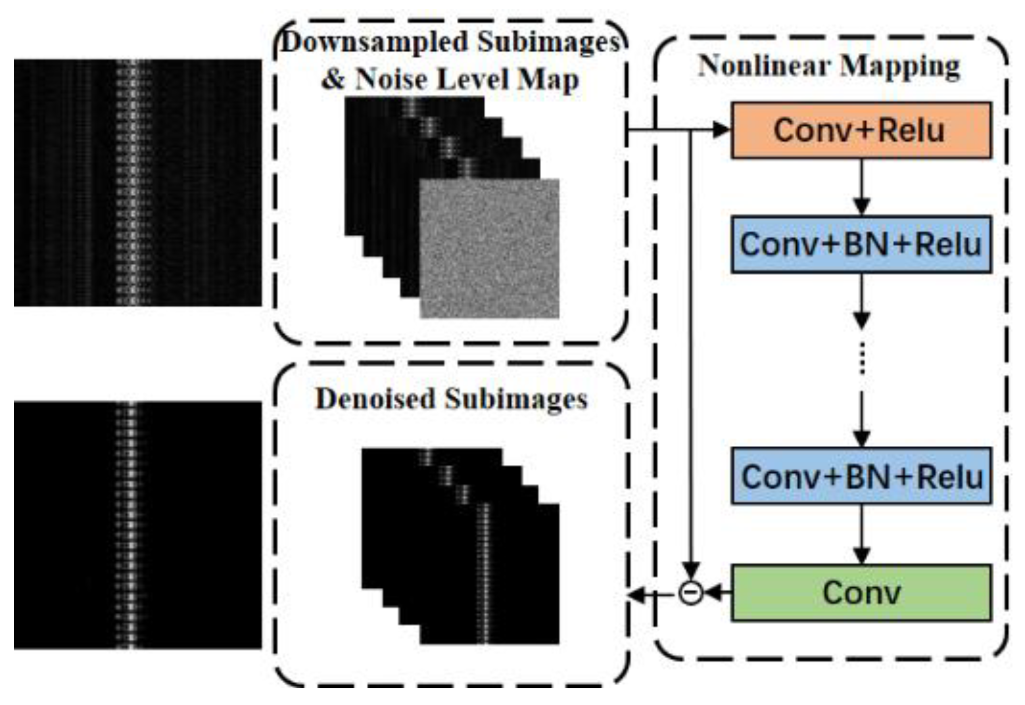
In this section, we describe a convolutional neural network capable of being used for image denoising, the FFDNet, which has the network structure shown in Figure 1. The first layer of the FFDNet network is a reversible downsampling operator that reduces the size of a noise image to four downsampled sub-images. The back part of the nonlinear mapping, consisting of a series of 3 × 3-pixel convolutional kernels. Each layer consists of three types of operations: Convolution (Conv), Rectified Linear Unit (ReLU), and Batch Normalization (BN). Specifically, the first layer consists of “Conv + ReLU”, the middle layer uses “Conv + BN + ReLU”, and the last layer contains only “Conv” for reconstructing the output. Zero padding is used after each convolution to ensure that the output image of each layer has the same scale as the input image. The last layer of the network uses an upsampling operation as an inverse of the downsampling operation of the first layer, resulting in an estimated clean image.
In terms of network structure, the FFDNet network model adds two sub-networks, image downsampling and sub-pixel convolution, which correspond to the red dashed box and green dashed box, respectively, in Figure 2. The downsampling factor is set to 2; therefore, the original noisy image with sizes W × H × C is reshaped into sub-images with sizes (W/2) × (H/2) × 4C through downsampling. Then, these sub-images are used as inputs to the network, which reduces the computational load per training iteration and increases the receptive field of the network for denoising the sub-images to some extent. After downsampling, the image size is reduced to half of the original size, and the receptive field of the network for the sub-image is equivalent to twice the size of the original image [28]. The increased receptive field can make the enabling range of image noise reduction larger, and the noise reduction will become more uniform, which helps to solve the problem of difficult local noise removal [26,29]. In addition, the increase in the number of sub-images increases the number of noise reduction network samples and enables more detailed noise reduction features to be learned [30,31]. The FFDNet network also feeds noise levels into the network for training along with the images and expands the noise levels to a noise level map with the same dimensionality as the input image. The introduction of the noise level map makes the network more flexible and increases the range of noise level perception by the noise reduction network. All the denoised low-resolution sub-images are then reconstructed into high-resolution denoised images by upsampling. Figure 2 provides a more intuitive view of how the input image changes in the network after downsampling and upsampling processing.
The nonlinear mapping of the FFDNet network applies three operations, convolution (Conv), BN, and ReLU activation functions, the principles of which are explained in detail here. The convolutional layer consists of several convolutional units, each with parameters optimized by a back-propagation algorithm [32]. The main purpose of the convolution operation is to extract the features of the image, which are represented by each pixel in the image in a combined or independent way, such as texture features and edge features [33]. During the training process, the parameters of each layer of the network directly affect the input distribution of the next layer of the network, which increases the time complexity of training the network. To speed up the training and convergence of the network, the batch normalization (BN) method is used to process small batches of samples extracted from sub-images [34].
The BN layer is located after the Conv layer and before the activation function. By introducing operations such as normalization and shifting, it forcibly pulls the distribution of the input data of each layer of the network back to a standard normal distribution with a mean of 0 and a variance of 1. The specific process of BN is as follows: First, the mean value and standard deviation of output data of the previous layer are calculated, which can be expressed as
where m is the batch size of this training sample. The obtained data are then normalized and can be expressed as
where ε is a constant very close to 0, added to avoid the denominator being zero. Finally, the data obtained from the above normalization processing is reconstructed, which can be obtained as follows.
where γ and β are the learning parameters of BN. BN allows the input values of the activation layer to fall in regions where the activation function is more sensitive to the input, which helps avoid the problem of gradient disappearance and speeds up the convergence of the network.
The output of the upper layer is applied to the activation function to obtain the input value of the next layer. The rectified linear unit (ReLU), as a nonlinear activation function, can improve the nonlinear fitting ability of the neural network and enhance the expression ability of the model, and the ReLU function can be expressed as
where x is the input number, and the gradient of ReLU can only take two values: 0 or 1, when x is less than 0, the gradient is 0; when x is greater than 0, the gradient is 1. Thus the concatenation of gradients of ReLU does not converge to zero, effectively alleviating the problem of vanishing gradients [35].
ReLU(x) = max(0, x)
3. FFDNet-Based Denoising Method
The FFDNet denoising network was first proposed by Zhang et al. and applied to image denoising [31,36]. This section details the process of pre-processing the vibration data, explains the dataset generation method, and elucidates the denoising process of the FFDNet network.
3.1. Vibration Data Preprocessing
The data collected typically include a data matrix consisting of the number of Rayleigh backscattered traces and the sampling points for each trace, with the horizontal direction of each matrix representing the spatial domain and the vertical direction representing the temporal domain [37]. The length of the data in the spatial domain is determined by the length of the sensing fiber, and the length in the temporal domain is 0.05 s and contains 500 Rayleigh backscattered traces, with each detection pulse acquiring one Rayleigh backscattered trace, as shown in Figure 3.
The data matrix contains the amplitude information of the vibration signal, and the data matrix is processed differentially according to the time series. In the case of no noise, the difference results of all adjacent time series except the vibration position are zero, and the position where the difference result is not zero is the vibration position located. The principle of vibration location can be referred to in the following formula.
where K is the number of Rayleigh backscattered traces collected and L is the number of points sampled on each trace. After differencing the data matrix, the differential matrix is obtained. Finally, the differential matrix is greyed out to obtain a greyscale image containing the vibration information, which is processed by a specific image denoising algorithm to achieve denoising of the Rayleigh backscattered traces. The grayscale images have two fewer channels than RGB images, and the reduced dimensionality allows convolutional neural networks to compute greyscale images faster. The processed data matrix for each event only represents the evolution of intensity over time at different spatial locations, while greyscale images are able to represent the relationship between intensity changes over time and space. Therefore, converting the processed data matrix to greyscale images can both preserve the useful signals in the data matrix intact and reduce the amount of computing. The complete data pre-processing process is shown in Figure 3.
3.2. FFDNet Image Denoising Process
Figure 4 demonstrates the process of denoising using the FFDNet network, which is divided into two parts: training and testing, each of which is described below.
The data set used for training the network is generated by computer, including the training set and the test set. In order to avoid overfitting or underfitting the trained network, the data set used should not be too small or too large [38]. Therefore, after several tests, the number of data sets was chosen to be 600 greyscale images, the size of the images was set to be 200 × 200. In these grayscale images, bright stripes with a width of 20 pixels were added to the dark background to simulate the ideal vibration signal of the φ-OTDR system. It should be noted that since the vibration position is random in reality, the bright stripes should also be generated at random positions. At the same time, in order to improve the recognition ability of the network for multiple vibration events, the training set was divided into three parts on average. One, two, and three bright stripes were added, respectively, with a width of 20 pixels and random positions. The test set is also divided into three parts to represent single and multiple events. The number of images in the training set and the test set are divided into a ratio of 3:1. AWGN is used to simulate the background noise of the φ-OTDR system, and AWGN was superimposed into the 600 gray images generated and sent to the training network together.
FFDNet incorporates the concept of residual learning by treating the denoising network as a residual module [32]. This approach involves directly transforming the network’s output into a residual image, assuming that the clean image is x, the noisy image is y, and the residual image is N, where N = y − x. By adopting this framework, FFDNet aims to improve the performance of denoising. The goal of the network to be optimized is not the mapping between the clean image and the network output but the mapping between the real residual image and the network output. The use of residual learning allows the network to learn more easily and the loss function to be optimized more efficiently than learning a clean image directly. The loss function can be expressed as follows.
where denotes the noise estimate of the network output, denotes the noise image, denotes the noise level map, and m denotes the number of patches of the input. The pre-processed noisy images are sent to the trained FFDNet model for noise estimation, and a clean image is an output based on the noise estimated by the FFDNet model.
4. Experimental Results and Analysis
4.1. Experimental Setup and Parameter Initialization
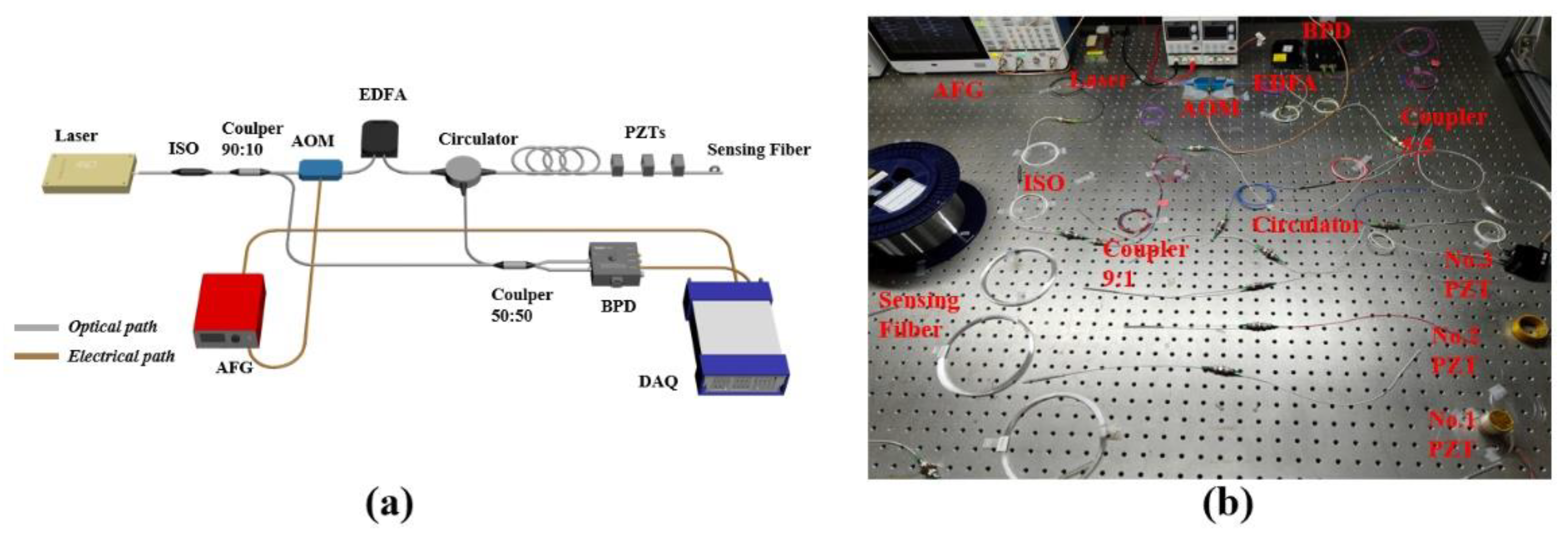
The φ-OTDR system based on coherent detection was used to verify the performance of the FFDNet network. A continuous laser of 1550 nm is generated from a laser with a linewidth of 3 kHz. The isolator (ISO) is added behind the light source to prevent the Rayleigh backscattered light from damaging the laser. The continuous laser is divided into two channels through a 90:10 coupler: one light is used as the reference light, and the other light is pulse modulated by an AOM with pulse width of 50 ns and repetition rate of 10 kHz. The AOM also introduces a frequency shift of 150 MHz to the light frequency. Then, the detection pulse is amplified by an erbium-doped fiber amplifier (EDFA) and injected into the 1.4 km sensing fiber through a circulator. Vibration signals generated by the piezoelectric ceramic transducer (PZT) are applied to the fiber. The backscatter signal and reference light returned along the sensing fiber are converted into electrical signals by a photodetector (BPD) through a 50:50 coupler and sampled by a data acquisition card (DAQ), which sampling rate is set at 625 MHz. The experimental apparatus is shown in Figure 5.
For the experimental validation, three piezoelectric ceramics were placed 100 m apart on 1.4 km sensing fiber to simulate disturbances at different locations in the real world.
In order to further verify the ability of the FFDNet network to identify different vibration intensities, we used a signal generator to apply different voltages to different piezoelectric ceramics as a means of adjusting the strength of the vibration signal to determine whether the FFDNet can accurately remove noise. At the same time, the proposed scheme is compared with the classical wavelet denoising scheme and Gaussian filtering scheme.
The system structure of FFDNet was described in Section 2.2 and is shown in Figure 1. Its network depth was set to 15, and the Adam algorithm was used to minimize the loss function during training, with its hyperparameters set to default values. We trained the network for 80 epochs, and in order to make the network converge faster and more stable, we used a decaying learning rate by setting the initial learning rate to 1 × 10³ and decreasing it by a factor of 0.1 every 30 epochs. The detailed hyperparameter initialization for FFDNet is shown in Table 1. The hardware environment used to train the FFDNet network model was a computer with a 10-core Intel(R) Core(TM) i9-10850K CPU @ 3.60 GHz, 16GBRAM, and an NVIDIA RTX3070 GPU. The software environment is a Windows 10 operating system. Training is based on a Python 3.6 environment and the PyTorch deep learning framework.
4.2. Comparison and Analy{Citation}sis of Experimental Results
The experimental setup for this experiment is shown in Figure 5. Piezoelectric ceramics were placed at 1170 m, 1270 m, and 1370 m, named PZT No.1, PZT No.2, and PZT No.3 by distance domain, respectively. In order to further demonstrate the robustness of FFDNet network denoising, the experiment was divided into three parts: the first experiment only applied 200 Hz vibration to PZT No.1; the second experiment selected PZT No.1 and PZT No.2 to apply 200 Hz vibration at the same time, the voltage was set to 3v and 2v, respectively; the third experiment applied 200 Hz vibration to three PZTs at the same time, the voltage was set to 1v, 3v and 2v, respectively. The effectiveness of the FFDNet network in single and multi-event denoising is verified by these experiments. Figure 6a–c shows the results of the original 500 Rayleigh backscattered traces after differencing. The peaks at 1170 m, 1270 m, and 1370 m, which correspond to the bright stripes in the greyscale image. However, as can be seen from the images, although the φ-OTDR system based on coherent detection was able to locate our artificially imposed vibration signal, the composite background noise at 1080~1120 m was still at a high level, leading to a pseudo peak in this range. The SNR dropped to around 8 dB for all three experiments. The SNR of the location information is described as
where and are the energy values of the signal voltage and the background noise voltage, respectively [39,40].
As shown in Figure 7, the trained FFDNet network effectively reduced the noise in the image. Despite this noise reduction, the vibration signal at the designated location remained intact. The figure demonstrates that the original vibration width was preserved for both single and multiple vibration events. This demonstrates that FFDNet can accurately identify vibration signals in complex environments and remove environmental noise with a high degree of robustness while retaining detailed information about the vibration signals.
After verifying the feasibility of FFDNet network denoising, the traditional denoising methods were also used to denoise the original differential data as a comparison with FFDNet network. Figure 8 and Figure 9 show the results after wavelet denoising and Gaussian filtering, respectively. Among the traditional denoising methods, they are generally divided into spatial domain methods and transform domain methods. Gaussian filter is a typical spatial domain method, while the most representative of the transform domain method is wavelet denoising. The wavelet denoising method carries out wavelet transform of the original signal, sets a coefficient threshold, i.e., below the threshold as a useful signal to retain and above the threshold as noise to remove, and finally reconstructs the signal to obtain the final result. We used the bior2.2 function as the wavelet basis function to decompose the original signal into four layers and filter it layer by layer with the threshold value. The original differential Rayleigh backscattered traces of the three experiments were denoised by wavelet denoising. The final denoised results of the three experiments are shown in Figure 8a–c. After wavelet denoising, the SNR is improved to about 11 dB, while the details of the original signal are preserved. However, although the SNR of the system is improved after wavelet denoising, there are still obvious pseudo peaks between 1080 and 1120 m. The other traditional denoising method we have chosen is Gaussian filtering. It is the process of weighted averaging over the entire image, where the value of each pixel point is obtained by a weighted average of its own and other pixel values in its neighborhood. The specific operation of Gaussian filtering is that a Gaussian filter template is used to scan each pixel in the image, and use the weighted average gray value of the pixels in the neighborhood determined by the template to replace the value of the central pixel of the template. The original differential Rayleigh backscatter traces from these three experiments were denoised by Gaussian filter using a 5 × 5 template, and the final denoised results of the three experiments are shown in Figure 9a–c, where the SNR of the system is improved to about 11 dB. Similarly, it can be seen from the result that although the SNR of the system is improved compared with that without denoising, the pseudo peaks still exist within 1080~1120 m. For the two traditional denoising methods, both the transform domain method and the spatial domain method will have the phenomenon of not being able to remove the pseudo peaks, which does not fully meet the needs of the φ-OTDR system. The experimental results have proven that compared to the deep learning denoising methods, the traditional denoising methods still exist some limitations.
The comparison of SNR improvement of the three denoising methods is shown in Figure 10. It can be seen that the denoising scheme based on FFDNet network greatly improves the SNR of the system, up to 37.84 dB. In general, compared with the traditional denoising methods, the proposed denoising scheme has the characteristics of high SNR and high robustness and has high potential in practical applications.
5. Conclusions
In this paper, an FFDNet based denoising method is proposed to improve the SNR of vibration measurements in φ-OTDR systems. The noise removal of multiple vibration events at different locations is achieved, and the SNR of the vibration source’s location information is improved to 37.84 dB, 37.11 dB, and 37.31 dB in single-event, dual-event, and multi-event experiments, respectively, which verifies the performance of the proposed denoising method. Compared with transform domain denoising methods and spatial domain denoising methods (such as wavelet denoising and Gaussian filtering), the deep learning based denoising method (FFDNet) can better improve the SNR system and more effectively preserve the vibration signals details. Therefore, the FFDNet based denoising method has proved to be a potential solution to improve the performance of the φ-OTDR system and enhance its ability to recognize multi-vibration events.
Author Contributions
Conceptualization, X.Y., S.L. and Z.Q.; methodology, X.Y.; software, X.Y.; validation, X.Y., S.L., Y.X., Z.L. and Z.Q.; formal analysis, X.Y. and Y.X.; investigation, X.Y. and S.L.; resources, Z.L., Z.Q. and Y.X.; data curation, X.Y. and S.L.; writing—original draft preparation, X.Y.; writing—review and editing, X.Y., S.L. and Z.Q.; visualization, X.Y.; supervision, Y.X. and Z.Q.; project administration, Z.L. and Z.Q. All authors have read and agreed to the published version of the manuscript.
Funding
Natural Science Foundation of Shandong Province (ZR2020MF110, ZR2020MF118); Shandong Provincial Key Research and Development Program (Major Scientific and Technological Innovation Project) (2020CXGC010204); Qilu Young Scholar Program of Shandong University.
Institutional Review Board Statement
Not applicable.
Informed Consent Statement
Not applicable.
Data Availability Statement
Data underlying the results presented in this paper are not publicly available at this time but may be obtained from the authors upon reasonable request.
Acknowledgments
The research results of this article would not have been accomplished without the guidance of the author’s supervisor, the help of fellow students, and the support of the research group’s professors. The author sincerely appreciates the excellent experimental environment they provided.
Conflicts of Interest
The authors declare no conflict of interest.
References
- Lu, Y.; Zhu, T.; Chen, L.; Bao, X. Distributed Vibration Sensor Based on Coherent Detection of Phase-OTDR. J. Light. Technol. 2010, 28, 5585644. [Google Scholar] [CrossRef]
- Zhang, Z.; Bao, X. Distributed Optical Fiber Vibration Sensor Based on Spectrum Analysis of Polarization-OTDR System. Opt. Express 2008, 16, 10240. [Google Scholar] [CrossRef] [PubMed]
- Qin, Z.; Zhu, T.; Chen, L.; Bao, X. High Sensitivity Distributed Vibration Sensor Based on Polarization-Maintaining Configurations of Phase-OTDR. IEEE Photon. Technol. Lett. 2011, 23, 1091–1093. [Google Scholar] [CrossRef]
- Wu, H.; Wang, Z.; Peng, F.; Peng, Z.; Li, X.; Wu, Y.; Rao, Y. Field Test of a Fully Distributed Fiber Optic Intrusion Detection System for Long-Distance Security Monitoring of National Borderline; López-Higuera, J.M., Jones, J.D.C., López-Amo, M., Santos, J.L., Eds.; SPIE: Bellingham, WA, USA, 2014; p. 915790. [Google Scholar]
- Peng, F.; Wu, H.; Jia, X.-H.; Rao, Y.-J.; Wang, Z.-N.; Peng, Z.-P. Ultra-Long High-Sensitivity Φ-OTDR for High Spatial Resolution Intrusion Detection of Pipelines. Opt. Express 2014, 22, 13804. [Google Scholar] [CrossRef]
- Tejedor, J.; Ahlen, C.H.; Gonzalez-Herraez, M.; Macias-Guarasa, J.; Martins, H.F.; Pastor-Graells, J.; Martin-Lopez, S.; Guillen, P.C.; De Pauw, G.; De Smet, F.; et al. Real Field Deployment of a Smart Fiber-Optic Surveillance System for Pipeline Integrity Threat Detection: Architectural Issues and Blind Field Test Results. J. Light. Technol. 2018, 36, 1052–1062. [Google Scholar] [CrossRef]
- Wu, H.; Qian, Y.; Zhang, W.; Tang, C. Feature Extraction and Identification in Distributed Optical-Fiber Vibration Sensing System for Oil Pipeline Safety Monitoring. Photonic Sens 2017, 7, 305–310. [Google Scholar] [CrossRef]
- Lv, A.; Li, J. On-Line Monitoring System of 35 kV 3-Core Submarine Power Cable Based on φ-OTDR. Sens. Actuators A Phys. 2018, 273, 134–139. [Google Scholar] [CrossRef]
- Muanenda, Y. Recent Advances in Distributed Acoustic Sensing Based on Phase-Sensitive Optical Time Domain Reflectometry. J. Sens. 2018, 2018, 3897873. [Google Scholar] [CrossRef]
- Shi, Y.; Feng, H.; Zeng, Z. Distributed Fiber Sensing System with Wide Frequency Response and Accurate Location. Opt. Lasers Eng. 2016, 77, 219–224. [Google Scholar] [CrossRef]
- Chen, M.; Masoudi, A.; Brambilla, G. Performance Analysis of Distributed Optical Fiber Acoustic Sensors Based on φ-OTDR. Opt. Express 2019, 27, 9684. [Google Scholar] [CrossRef]
- Li, S.; Qin, Z.; Liu, Z.; Yang, W.; Qu, S.; Wang, Z.; Xu, Y. Long-Distance Φ-OTDR with a Flexible Frequency Response Based on Time Division Multiplexing. Opt. Express 2021, 29, 32833. [Google Scholar] [CrossRef]
- Ren, M.; Lu, P.; Chen, L.; Bao, X. Theoretical and Experimental Analysis of O-OTDR Based on Polarization Diversity Detection. IEEE Photon. Technol. Lett. 2016, 28, 697–700. [Google Scholar] [CrossRef]
- Li, D.; Wang, H.; Wang, X.; Li, X.; Huang, T.; Ge, M.; Yin, J.; Chen, S.; Huang, B.; Guan, K.; et al. Denoising Algorithm of Φ -OTDR Signal Based on Curvelet Transform with Adaptive Threshold. Opt. Commun. 2023, 545, 129708. [Google Scholar] [CrossRef]
- Jousset, P.; Reinsch, T.; Ryberg, T.; Blanck, H.; Clarke, A.; Aghayev, R.; Hersir, G.P.; Henninges, J.; Weber, M.; Krawczyk, C.M. Dynamic Strain Determination Using Fibre-Optic Cables Allows Imaging of Seismological and Structural Features. Nat. Commun. 2018, 9, 2509. [Google Scholar] [CrossRef]
- Lu, B.; Wu, B.; Gu, J.; Yang, J.; Gao, K.; Wang, Z.; Ye, L.; Ye, Q.; Qu, R.; Chen, X.; et al. Distributed Optical Fiber Hydrophone Based on Φ-OTDR and Its Field Test. Opt. Express 2021, 29, 3147. [Google Scholar] [CrossRef]
- Shang, Y.; Sun, M.; Wang, C.; Yang, J.; Du, Y.; Yi, J.; Zhao, W.; Wang, Y.; Zhao, Y.; Ni, J. Research Progress in Distributed Acoustic Sensing Techniques. Sensors 2022, 22, 6060. [Google Scholar] [CrossRef]
- Zabihi, M.; Chen, Y.; Zhou, T.; Liu, J.; Shan, Y.; Meng, Z.; Wang, F.; Zhang, Y.; Zhang, X.; Chen, M. Continuous Fading Suppression Method for Φ-OTDR Systems Using Optimum Tracking Over Multiple Probe Frequencies. J. Light. Technol. 2019, 37, 3602–3610. [Google Scholar] [CrossRef]
- Yu, Z.; Lu, Y.; Hu, X.; Meng, Z. Polarization Dependence of the Noise of Phase Measurement Based on Phase-Sensitive OTDR. J. Opt. 2017, 19, 125602. [Google Scholar] [CrossRef]
- Qin, Z.; Chen, L.; Bao, X. Continuous Wavelet Transform for Non-Stationary Vibration Detection with Phase-OTDR. Opt. Express 2012, 20, 20459. [Google Scholar] [CrossRef]
- Qin, Z.; Chen, L.; Bao, X. Wavelet Denoising Method for Improving Detection Performance of Distributed Vibration Sensor. IEEE Photon. Technol. Lett. 2012, 24, 542–544. [Google Scholar] [CrossRef]
- Qin, Z.; Chen, H.; Chang, J. Signal-to-Noise Ratio Enhancement Based on Empirical Mode Decomposition in Phase-Sensitive Optical Time Domain Reflectometry Systems. Sensors 2017, 17, 1870. [Google Scholar] [CrossRef] [PubMed]
- Qu, S.; Qin, Z.; Xu, Y.; Cong, Z.; Wang, Z.; Yang, W.; Liu, Z. High Spatial Resolution Investigation of OFDR Based on Image Denoising Methods. IEEE Sens. J. 2021, 21, 18871–18876. [Google Scholar] [CrossRef]
- He, H.; Shao, L.; Li, H.; Pan, W.; Luo, B.; Zou, X.; Yan, L. SNR Enhancement in Phase-Sensitive OTDR with Adaptive 2-D Bilateral Filtering Algorithm. IEEE Photonics J. 2017, 9, 1–10. [Google Scholar] [CrossRef]
- Liehr, S.; Borchardt, C.; Münzenberger, S. Long-Distance Fiber Optic Vibration Sensing Using Convolutional Neural Networks as Real-Time Denoisers. Opt. Express 2020, 28, 39311. [Google Scholar] [CrossRef]
- Krizhevsky, A.; Sutskever, I.; Hinton, G.E. ImageNet Classification with Deep Convolutional Neural Networks. Commun. ACM 2017, 60, 84–90. [Google Scholar] [CrossRef]
- Gao, X.; Hu, W.; Dou, Z.; Li, K.; Gong, X. A Method on Vibration Positioning of Φ-OTDR System Based on Compressed Sensing. IEEE Sens. J. 2022, 22, 16422–16429. [Google Scholar] [CrossRef]
- Wang, H.; Wang, Y.; Wang, X.; Wang, S.; Liu, T. A Novel Deep-Learning Model for RDTS Signal Denoising Based on Down-Sampling and Convolutional Neural Network. J. Light. Technol. 2022, 40, 3647–3653. [Google Scholar] [CrossRef]
- Zhang, K.; Zuo, W.; Gu, S.; Zhang, L. Learning Deep CNN Denoiser Prior for Image Restoration. In Proceedings of the 2017 IEEE Conference on Computer Vision and Pattern Recognition (CVPR), Honolulu, HI, USA, 26 July 2017; pp. 2808–2817. [Google Scholar]
- Shi, W.; Caballero, J.; Huszár, F.; Totz, J.; Aitken, A.P.; Bishop, R.; Rueckert, D.; Wang, Z. Real-Time Single Image and Video Super-Resolution Using an Efficient Sub-Pixel Convolutional Neural Network. In Proceedings of the IEEE Conference on Computer Vision and Pattern Recognition (CVPR), Las Vegas, NV, USA, 30 June 2016. [Google Scholar]
- Zhang, K.; Zuo, W.; Zhang, L. FFDNet: Toward a Fast and Flexible Solution for CNN-Based Image Denoising. IEEE Trans. Image Process. 2018, 27, 4608–4622. [Google Scholar] [CrossRef]
- Suresh, S.; Omkar, S.N.; Mani, V. Parallel Implementation of Back-Propagation Algorithm in Networks of Workstations. IEEE Trans. Parallel Distrib. Syst. 2005, 16, 24–34. [Google Scholar] [CrossRef]
- Murali, V.; Sudeep, P.V. Image Denoising Using DnCNN: An Exploration Study. In Advances in Communication Systems and Networks; Jayakumari, J., Karagiannidis, G.K., Ma, M., Hossain, S.A., Eds.; Lecture Notes in Electrical Engineering; Springer Singapore: Singapore, 2020; Volume 656, pp. 847–859. ISBN 9789811539916. [Google Scholar]
- Ioffe, S.; Szegedy, C. Batch Normalization: Accelerating Deep Network Training by Reducing Internal Covariate Shift. In Proceedings of the 32nd International Conference on Machine Learning, Lille, France, 6–11 July 2015. [Google Scholar]
- Yarotsky, D. Error Bounds for Approximations with Deep ReLU Networks. Neural Netw. 2017, 94, 103–114. [Google Scholar] [CrossRef]
- Tassano, M.; Delon, J.; Veit, T. An Analysis and Implementation of the FFDNet Image Denoising Method. Image Process. Line 2019, 9, 1–25. [Google Scholar] [CrossRef]
- Li, S.; Liu, K.; Jiang, J.; Xu, T.; Ding, Z.; Sun, Z.; Huang, Y.; Xue, K.; Jin, X.; Liu, T. An Ameliorated Denoising Scheme Based on Deep Learning for Φ-OTDR System With 41-Km Detection Range. IEEE Sens. J. 2022, 22, 19666–19674. [Google Scholar] [CrossRef]
- Yeom, S.; Giacomelli, I.; Fredrikson, M.; Jha, S. Privacy Risk in Machine Learning: Analyzing the Connection to Overfitting. In Proceedings of the 2018 IEEE 31st Computer Security Foundations Symposium (CSF), Oxford, UK, 9–12 July 2018; pp. 268–282. [Google Scholar]
- Fang, G.; Xu, T.; Feng, S.; Li, F. Phase-Sensitive Optical Time Domain Reflectometer Based on Phase-Generated Carrier Algorithm. J. Light. Technol. 2015, 33, 2811–2816. [Google Scholar] [CrossRef]
- Wang, Z.; Zhang, L.; Wang, S.; Xue, N.; Peng, F.; Fan, M.; Sun, W.; Qian, X.; Rao, J.; Rao, Y. Coherent Φ-OTDR Based on I/Q Demodulation and Homodyne Detection. Opt. Express 2016, 24, 853. [Google Scholar] [CrossRef]
Figure 1.
The architecture of the proposed FFDNet for image denoising. The input image is reduced to four sub-images. The output image is reconstructed from four denoised sub-images.
Figure 1.
The architecture of the proposed FFDNet for image denoising. The input image is reduced to four sub-images. The output image is reconstructed from four denoised sub-images.

Figure 2.
Diagram of downsampling and upsampling.

Figure 3.
Data preprocessing flow chart.

Figure 4.
Flow chart of the FFDNet-based denoising method.

Figure 5.
(a) Schematic diagram of the φ-OTDR system (b) Physical diagram of the φ-OTDR system (Laser: narrow linewidth semiconductor laser; ISO: isolator; AOM: acoustic-optic modulator; EDFA: erbium-doped fiber amplifier; FUT: fiber under test. PZT: piezoelectric ceramic transducer; BPD: balanced photodetector; DAQ: data acquisition card; AFG: arbitrary function generator.).

Figure 6.
Differential processing of raw Rayleigh backscatter traces: (a) single-event, (b) dual-event, and (c) multi-event.
Figure 6.
Differential processing of raw Rayleigh backscatter traces: (a) single-event, (b) dual-event, and (c) multi-event.

Figure 7.
Differential Rayleigh backscattered traces denoised by the trained FFDNet network: (a) single-event, (b) dual-event, and (c) multi-event.
Figure 7.
Differential Rayleigh backscattered traces denoised by the trained FFDNet network: (a) single-event, (b) dual-event, and (c) multi-event.

Figure 8.
Differential Rayleigh backscattered traces after wavelet denoising: (a) single-event, (b) dual-event, and (c) multi-event.
Figure 8.
Differential Rayleigh backscattered traces after wavelet denoising: (a) single-event, (b) dual-event, and (c) multi-event.

Figure 9.
Differential Rayleigh backscattered traces after Gaussian filtering: (a) single-event, (b) dual-event, and (c) multi-event.
Figure 9.
Differential Rayleigh backscattered traces after Gaussian filtering: (a) single-event, (b) dual-event, and (c) multi-event.

Figure 10.
SNR of single-event and multi-event vibration position information obtained by three methods at 200 Hz.
Figure 10.
SNR of single-event and multi-event vibration position information obtained by three methods at 200 Hz.


Table 1.
FFDNet hyperparameter initialization.
| Hyperparameters | Initial Value |
|---|---|
| Weight Initialization | 1 |
| Bias Initialization | 0 |
| Learning Rate | 0.001 (0.1× decrease for every 30 epoch) |
| Epoch | 80 |
| Batch size | 128 |
Disclaimer/Publisher’s Note: The statements, opinions and data contained in all publications are solely those of the individual author(s) and contributor(s) and not of MDPI and/or the editor(s). MDPI and/or the editor(s) disclaim responsibility for any injury to people or property resulting from any ideas, methods, instructions or products referred to in the content. |
© 2023 by the authors. Licensee MDPI, Basel, Switzerland. This article is an open access article distributed under the terms and conditions of the Creative Commons Attribution (CC BY) license (https://creativecommons.org/licenses/by/4.0/).
Share and Cite
MDPI and ACS Style
Yang, X.; Li, S.; Xu, Y.; Liu, Z.; Qin, Z. Multi-Event Location Denoising Scheme for φ-OTDR Based on FFDNet Network. Photonics 2023, 10, 1114. https://0-doi-org.brum.beds.ac.uk/10.3390/photonics10101114
AMA Style
Yang X, Li S, Xu Y, Liu Z, Qin Z. Multi-Event Location Denoising Scheme for φ-OTDR Based on FFDNet Network. Photonics. 2023; 10(10):1114. https://0-doi-org.brum.beds.ac.uk/10.3390/photonics10101114
Chicago/Turabian StyleYang, Xiyu, Shuai Li, Yanping Xu, Zhaojun Liu, and Zengguang Qin. 2023. "Multi-Event Location Denoising Scheme for φ-OTDR Based on FFDNet Network" Photonics 10, no. 10: 1114. https://0-doi-org.brum.beds.ac.uk/10.3390/photonics10101114
Note that from the first issue of 2016, this journal uses article numbers instead of page numbers. See further details here.