Linear Combinations of the Complex Degrees of Coherence


1
Department of Physics, Huzhou University, Huzhou 313000, China
2
Sci-Tech School, Huzhou College, Huzhou 313000, China
3
Department of Physics, University of Miami, Coral Gables, FL 33146, USA
*
Author to whom correspondence should be addressed.
Photonics 2021, 8(5), 146; https://0-doi-org.brum.beds.ac.uk/10.3390/photonics8050146
Submission received: 1 April 2021
/
Revised: 25 April 2021
/
Accepted: 26 April 2021
/
Published: 28 April 2021
(This article belongs to the Special Issue Structured Light Coherence)
Abstract
:We propose a method for structuring the spatial coherence state of light via mixed linear combinations of N complex degrees of coherence (CDC) and specify the conditions under which such combinations represent a valid CDC. Several examples demonstrate that this method opens previously unknown avenues for modeling random sources, radiating to light fields with unique features.
1. Introduction
Various mathematical operations on the cross-spectral densities (CSDs) or the degrees of coherence can be used for modeling new partially coherent sources that radiate fields exhibiting exotic phenomena in their free-space evolution [1,2]. The most typical example of such a model is the multi-Gaussian Schell-model source, whose degree of coherence is represented as the linear combination of the sign-alternating Gaussian Schell-like correlation functions that generate far fields with flat intensity profiles [3]. More generally, the difference between any two CSDs belonging to the same correlation class has been proven to produce a valid CSD provided a certain sufficiency condition is satisfied [4,5]. In addition, the conditions under which the alternating series of any N CSDs pertaining to the same correlation class furnishes a valid CSD have also been elucidated [6]. In all these developments, the linear combinations were applied to the real-valued source correlation functions, producing far-fields with axial or Cartesian symmetries.
The spatial coherence state of light is generally a complex-valued function. The phase structure generally plays a very important role in characterization and propagation of the optical fields [7], and has a wide range of applications in optical imaging, particle manipulation, information transfer, laser communication, crystallography and photovoltaics [8,9,10,11,12,13,14]. Recently, a simple procedure based on the auto-convolution of a legitimate sliding function for modeling the Schell-like complex degree of coherence (CDC) with non-trivial phase profiles was proposed in [15], and was used to construct various genuine scalar and electromagnetic CDCs [16,17,18,19]. The results based on the sliding function modeling illustrate that various space-dependent phase profiles of the CDCs result in the far-field spectral density patterns with broken axial or Cartesian symmetries.
It was also illustrated that a sum of N non-negative CDCs with weighted linear phases belonging to the same class can yield the radiated fields of the same complexity as those previously achieved only with analytically intractable nonlinear phases, an example being an asymmetric spatial coherence grating or lattice [20]. However, the appearance of the negative terms in the linear combinations of the CDCs requires that additional conditions stemming from the nonnegative definiteness property of the CSD are met. In this paper, we tackle a problem of establishing sufficient conditions for constructing new, legitimate CDCs by combining the sums and the differences of the N complex-valued CDCs. We will illustrate by several examples that this method can lead to novel source coherence states producing unique far-field spectral density features.
2. Proposition
We set a CSD in the form of a weighted linear combination of the sum and the difference of N CSDs:
where are the positive weight constants and is the normalization coefficient. A single genuine CSD can be written as a superposition integral of the form [21]:
where is the non-negative function and is the arbitrary kernel. If N CSDs belong to the same correlation class, they possess the same kernel function . Then, Equation (1) can be represented as
where:
The necessary and sufficient condition ensuring the non-negative definiteness of the kernel in Equation (3) is that is a nonnegative function, meaning that:
For the Schell-model sources, takes the form [21]:
Additionally, hence Equation (3) becomes:
where is a profile function, and is the CDC defined as a function of a difference between two points, , being a Fourier transform pair of , i.e., . Then, the CDC can be expressed as
Let us set with a Cartesian phase in the form [15]:
where is the r.m.s. correlation width and is real constant. The CDC obtained on substituting from Equation (9) into Equation (8) takes the form:
where:
Furthermore, the corresponding far-field profile function , being the Fourier transform of , then takes the form:
3. Examples
3.1. Difference between Two CDCs
Let us now demonstrate the applications of this method with several numerical examples. The first one is the difference between two CDCs, i.e., and , then, the CDC and the corresponding far-field profile function take the following forms, respectively:
when the values of and are close, the necessary and sufficient conditions for the non-negative definiteness of Equation (14) are:
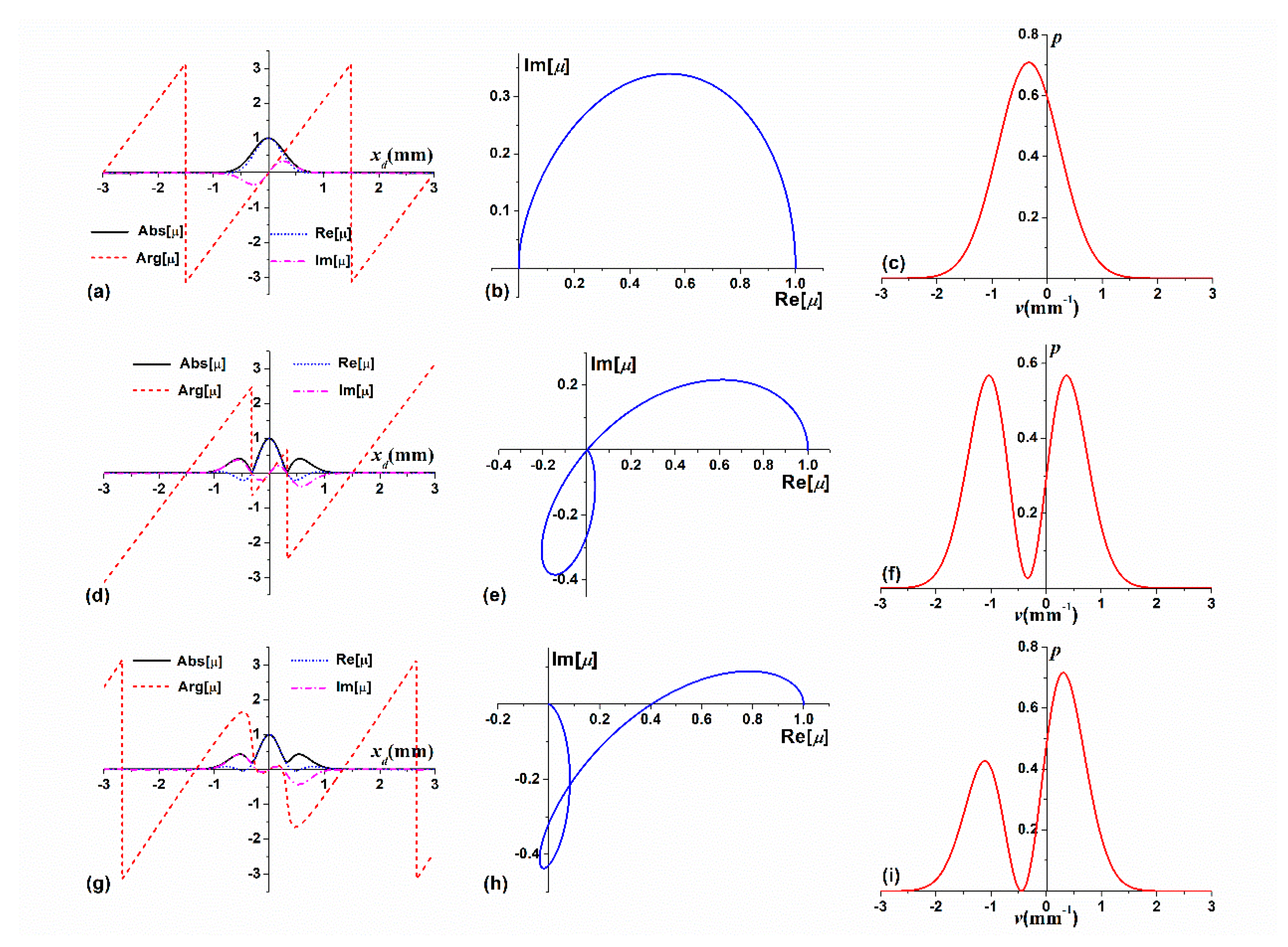
Figure 1 shows the numerical calculations relating to the complex coherence state and the far-field spectral density, plotted from Equations (13) and (14), respectively, for , and different values of the source parameters and . The subfigure in the left column, (a,d,g), the absolute value, the argument, the real part, and the imaginary part of the CDC are plotted against the separation distance . The subfigure in the middle column, (b,e,h), correspond to the left column presenting the coherence curves of these states. The subfigure in the right column, (c,f,j), illustrate the corresponding far-field spectral densities. The arrangement of other figures in this paper is the same as that in Figure 1. The first row, (a–c), shows the case of two CSDs with the same values of coherence length and the phase parameter , resulting in a laterally shifted Gaussian profile. When the values of the coherence length are different, the spectral density is split equally for the same values of the phase parameter as shown in the second row (d–f), or split unequally for a different , as shown in the last row (g–i):
3.2. Combination of Four CDCs
We then considered an example involving the combination of four CDCs when and . If we set , , , , and , then the CDC and the corresponding far-field profile function become:
From Equation (5), the constraint of non-negative definiteness can be expressed as
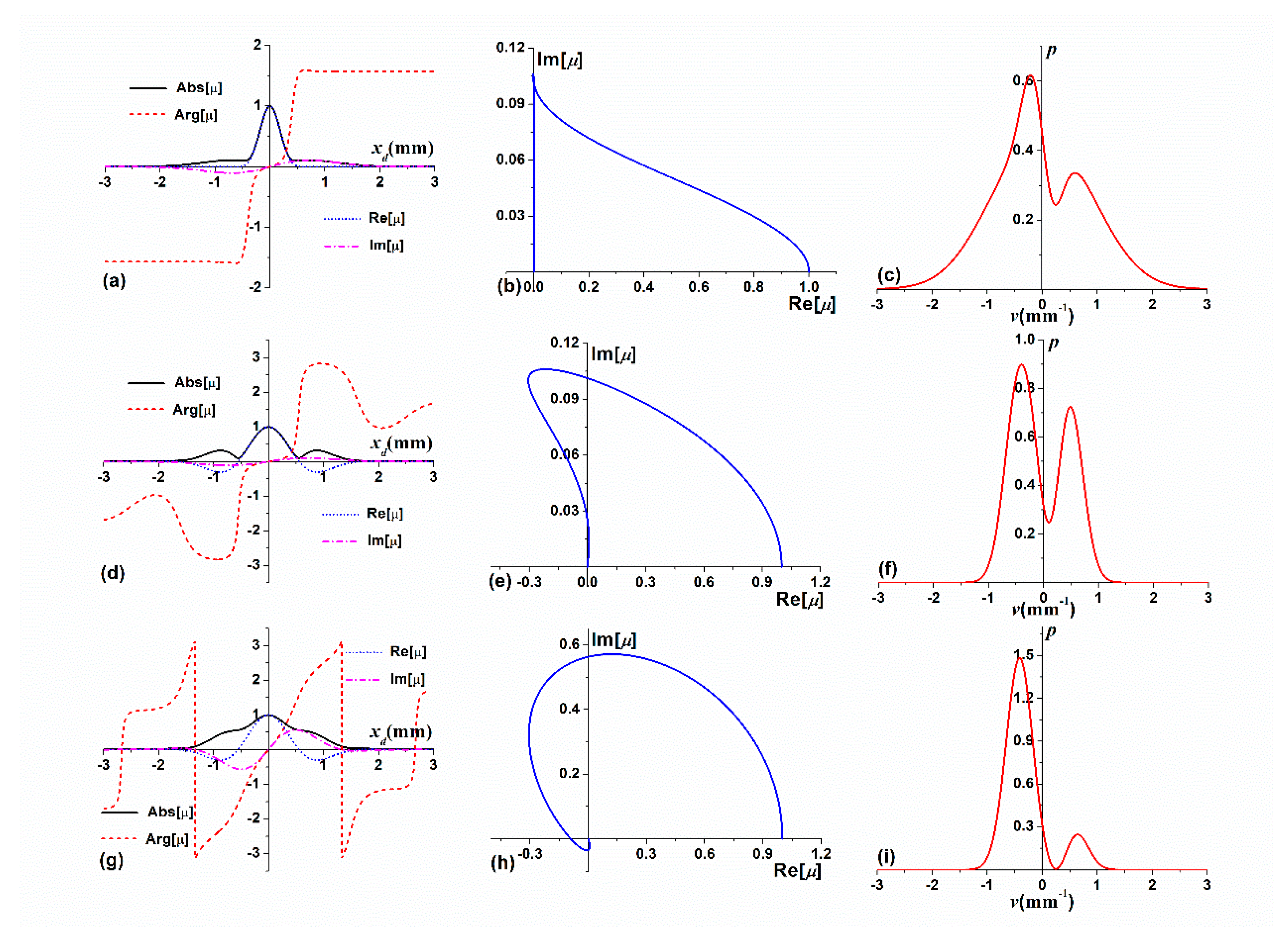
Figure 2 illustrates the source coherence states given in Equation (16) and the corresponding far-field spectral densities plotted from Equation (17) for , and different values of the source parameters , and . The first row of Figure 2 shows the case with , , and . The curves of the magnitude and phase are rather smooth, not involving substantial oscillations. The coherence curve is located in the first quadrant and the imaginary part is small. The far-field spectral density profile shows a partial split. In the second row of Figure 2, is close to the value of and the values of other parameters remain unchanged. In this case, the changes in the coherence curve and the splitting of the far-field spectral density become more substantial. In the bottom row of Figure 2 and the values of other parameters are the same as in the second row. The magnitude of the CDC forms a wide distribution, the phase jumps occur at its edge, and the coherence curve presents a spiral shape with single loop.
When and , Equations (16)–(18) have the following form:
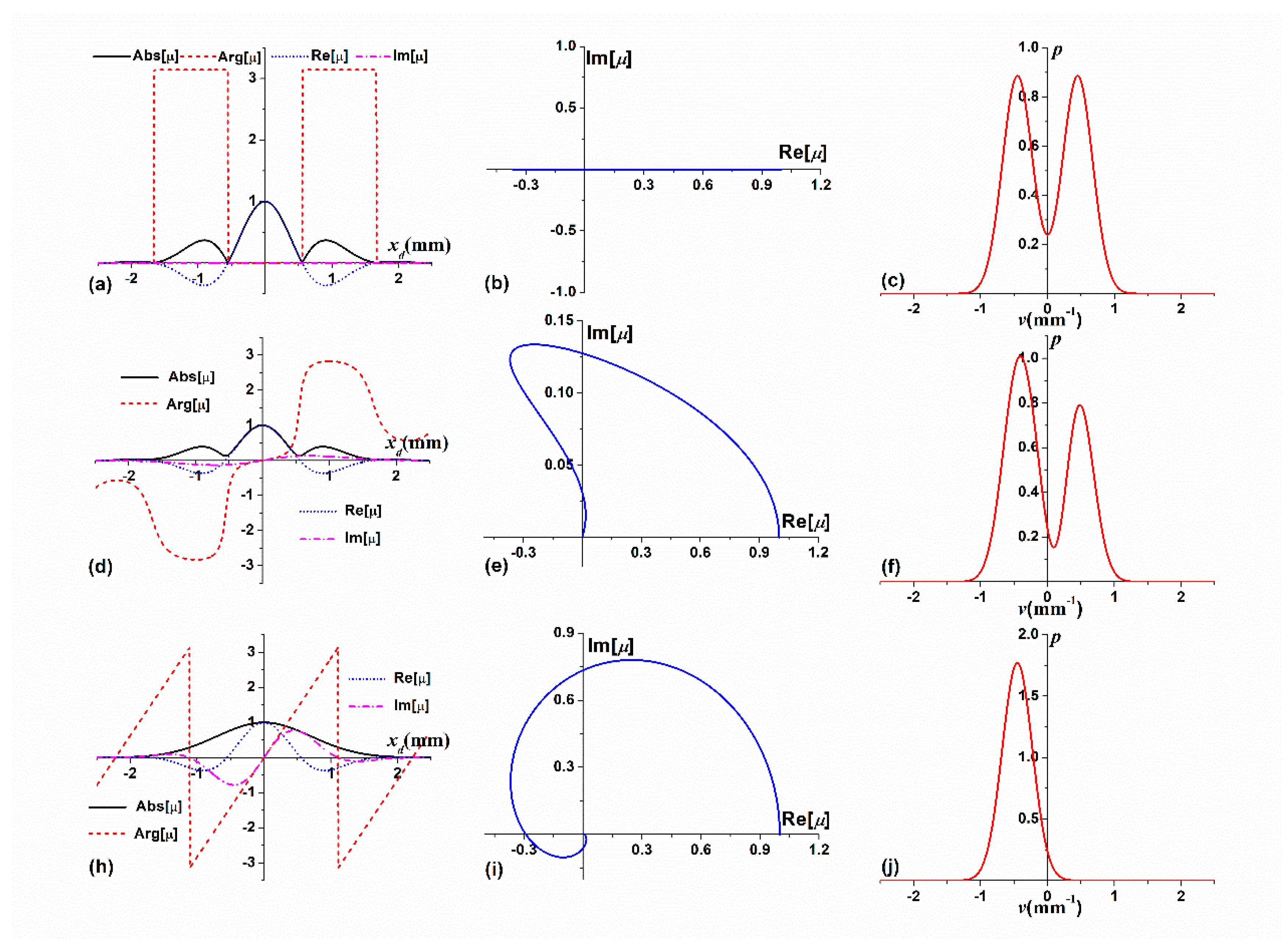
Figure 3 presents the numerical curves of the complex coherence state formation and the corresponding far-field spectral density distributions calculated form Equations (19) and (20) with and , respectively, for different values of the parameters and . Without phase modulation, i.e., , the first row of Figure 3 corresponds to the cosine–Gaussian correlation model [22]. The far-field spectral density is split symmetrically with respect to the optical axis. As the value of increases the phase modulation of the coherence state and the far-field spectral density’s asymmetry strengthens gradually, as shown in the second row of Figure 3: the right lobe is suppressed and the left lobe is enhanced. When , as shown in the last row of Figure 3, the complex coherent state is equivalent to one with a linear phase. The right lobe of the far-field spectral density disappears completely, forming an off-axis Gaussian shape.
3.3. Series Combination of CDCs
Let us finally consider a series combination of CDCs, setting and , whose phases vary with the number of terms, i.e., , , where is a constant. The CDC, the corresponding far-field profile function and the constraint of nonnegative definiteness then become:
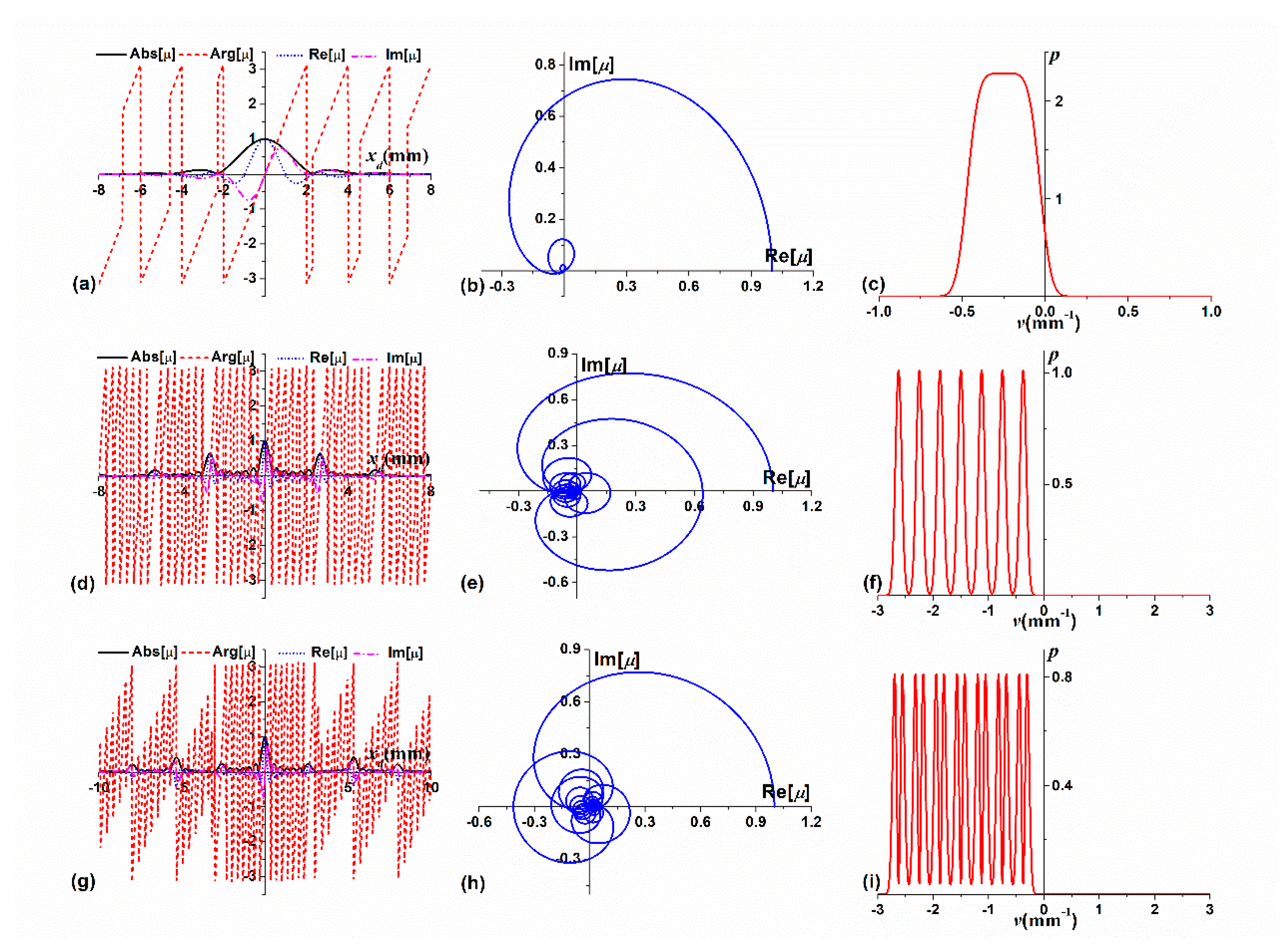
The numerical results for , , and different values of the parameters , and are shown in Figure 4. The first row of Figure 4 shows the case where and have the same value for all items and the values of is small. The CDC resembles a multi-Gaussian Schell-model case [18], the coherence curve presents a spiral-like cochleoid profile, and the far-field spectral density becomes a laterally shifted flat-top profile. As can be seen from the second row of Figure 4 for large values of , the CDC oscillates more, the spiral coherence curve is more complex, and presents a comb profile on one side of the optical axis. If the values of and are not equal, as shown in the third row of Figure 4, the teeth of the comb profile become denser.
4. Discussion: Correlation Linear Phase Plates
In the preceding theoretical analysis the intricate effects of a non-linear phase function of the source degree of coherence were shown to be mimicked by an incoherent superposition of several degrees of coherence with different linear phase functions. This brings us to the idea of introducing a new physical device of correlation optics, being a thin transmitting transparency (or, alternatively, a reflecting surface) with a 1D random slope distribution. A typical realization of this kind can be drawn from the ensemble of realizations having the phase part of the correlation function given in Equation (9).
Then, a linear CDC thin phase plate can be constructed as a physical optics device, similarly to the well-known ground glass diffusing plate, which only modifies the magnitude of the CDC in Equation (9) [23]. Recall that the rotation of the diffuser enables averaging over the formed ensemble of realizations of the random surface heights of the ground glass plate. However, unlike the diffuser, which uses the convenience of the Gaussian height (and, hence, width) statistics, the linear phase plate must be 3D manufactured from an optically highly transparent material having on one side the prescribed random slopes drawn from the ensemble with linear phase correlation in Equation (9). The thin plate then can be composed as a stack of narrow strips all having different slope realizations varying along one Cartesian direction, say x, and placed together along the other direction, say y. Therefore, dimension y can be used for generating the ensemble of 1D realizations. To achieve the ensemble averaging, the plate can be slid across the incident laser beam cross-section, in the y direction.
For the 2D control, the sequential application of two 1D plates can be made. Furthermore, for the generation of the non-linear phase CDC effects, the incoherent superposition of the linear phase CDC states is required, which can be achieved interferometrically.
The application of the coherence linear phase (slope) plates or their combinations at the source plane can be then used for the efficient statistical control of the radiated field in cases when asymmetric (in the axial or the Cartesian sense) far-field spectral density distributions are desired, the source must be portable and most of the power must be preserved. A current standard procedure involves expensive, cumbersome and optical power dispersing (to high diffraction modes) spatial light modulators mostly suitable for the laboratory operation [24]. Thus, our proposed approach suggests a promising procedure for analytical, and potentially practical, stationary optical field manipulation.
5. Concluding Remarks
In summary, we have examined the problem of constructing the linear combinations of the sum and the difference of N CDCs and established the corresponding conditions for obtaining new, legitimate, and stationary source models. Several numerical examples were included to illustrate the different possibilities that the linear combinations of the sums and the differences of the individual CDCs provide for developing new classes of random sources. All the examples show that such model sources generate unique and finely controllable far-field spectral densities.
Not only does the application of the linear phase function as a building blocks for various complex-valued CDC distributions, which gives insight into the structure of the very intricate coherence states, but it also provides a practical method for the simple experimental realization of the complex-valued CDC states. We have briefly suggested the use of the pre-manufactured rough surfaces with the well-chosen slope distributions for the generation of the 1D ensembles of realizations of the stationary sources with tunable linear CDC phases.
Author Contributions
Conceptualization, Z.M. and O.K.; methodology, Z.M. and O.K.; investigation, Z.M. and O.K.; writing—original draft preparation, Z.M.; writing—review and editing, O.K.; supervision, O.K.; project administration, Z.M.; funding acquisition, Z.M. All authors have read and agreed to the published version of the manuscript.
Funding
National Natural Science Foundation of China (NSFC) (Grant No. 11974107).
Institutional Review Board Statement
Not applicable.
Informed Consent Statement
Not applicable.
Data Availability Statement
No new data were created or analyzed in this study. Data sharing is not applicable to this article.
Conflicts of Interest
The authors declare no conflict of interest.
References
- Mandel, L.; Wolf, E. Optical Coherence and Quantum Optics; Cambridge University: Cambridge, UK, 1995. [Google Scholar]
- Korotkova, O. Random Beams: Theory and Applications; CRC Press: Boca Raton, FL, USA, 2013. [Google Scholar]
- Sahin, S.; Korotkova, O. Light sources generating far fields with tunable flat profiles. Opt. Lett. 2012, 37, 2970–2972. [Google Scholar] [CrossRef] [PubMed]
- Santarsiero, M.; Piquero, G.; de Sande, J.C.G.; Gori, F. Difference of cross-spectral densities. Opt. Lett. 2014, 39, 1713–1716. [Google Scholar] [CrossRef] [PubMed]
- Gori, F.; Santarsiero, M. Difference of two Gaussian Schell-model cross-spectral densities. Opt. Lett. 2014, 39, 2731–2734. [Google Scholar] [CrossRef] [PubMed]
- Mei, Z.; Korotkova, O. Alternating series of cross-spectral densities. Opt. Lett. 2015, 40, 2473–2476. [Google Scholar] [CrossRef] [PubMed]
- Wolf, E. Significance and measurability of the phase of a spatially coherent optical field. Opt. Lett. 2003, 28, 5–6. [Google Scholar] [CrossRef] [PubMed]
- Gbur, G.; Visser, T.D. Coherence vortices in partially coherent beams. Opt. Commun. 2003, 222, 117–125. [Google Scholar] [CrossRef]
- Wolf, E. Solution of the phase problem in the theory of structure determination of crystals from x-ray diffraction experiments. Phys. Rev. Lett. 2009, 103, 075501. [Google Scholar] [CrossRef] [PubMed] [Green Version]
- Popescu, G. Quantitaive Phase Imaging of Cells and Tissues; McGraw-Hill: New York, NY, USA, 2011. [Google Scholar]
- Ng, J.; Lin, Z.; Chan, C.T. Theory of optical trapping by an optical vortex beam. Phys. Rev. Lett. 2010, 104, 103601. [Google Scholar] [CrossRef] [PubMed] [Green Version]
- Wang, J. Advances in communications using optical vortices. Photon. Res. 2016, 4, B14–B28. [Google Scholar] [CrossRef]
- Nagali, E.; Sciarrino, F.; De Martini, F.; Marrucci, L.; Piccirillo, B.; Karimi, E.; Santamato, E. Quantum information transfer from spin to orbital angular momentum of photons. Phys. Rev. Lett. 2009, 103, 013601. [Google Scholar] [CrossRef] [PubMed] [Green Version]
- Divitt, S.; Novotny, L. Spatial coherence of sunlight and its implications for light management in photovoltaics. Optica 2015, 2, 95–103. [Google Scholar] [CrossRef]
- Korotkova, O.; Chen, X. Phase structuring of the complex degree of coherence. Opt. Lett. 2018, 43, 4727–4730. [Google Scholar] [CrossRef] [PubMed]
- Chen, X.; Korotkova, O. Complex degree of coherence modeling with famous planar curves. Opt. Lett. 2018, 43, 6049–6052. [Google Scholar] [CrossRef] [PubMed]
- Chen, X.; Korotkova, O. Phase structuring of the 2D complex coherence states. Opt. Lett. 2019, 44, 2470–2473. [Google Scholar] [CrossRef] [PubMed]
- Korotkova, O. Multi-Gaussian Schell-model source with a complex coherence state. J. Opt. 2019, 21, 045607. [Google Scholar] [CrossRef]
- Korotkova, O.; Chen, X.; Setälä, T. Electromagnetic Schell-model beams with arbitrary complex correlation states. Opt. Lett. 2019, 44, 4945–4949. [Google Scholar] [CrossRef] [PubMed]
- Mei, Z.; Korotkova, O. Asymmetric coherence gratings. Opt. Lett. 2020, 45, 1366–1369. [Google Scholar] [CrossRef] [PubMed]
- Gori, F.; Santarsiero, M. Devising genuine spatial correlation functions. Opt. Lett. 2007, 32, 3531–3533. [Google Scholar] [CrossRef] [PubMed] [Green Version]
- Mei, Z.; Korotkova, O. Cosine-Gaussian Schell-model sources. Opt. Lett. 2013, 38, 2578–2580. [Google Scholar] [CrossRef] [PubMed]
- Goodman, J.W. Statistical Optics; John Wiley & Sons: Hoboken, NJ, USA, 2015. [Google Scholar]
- Hyde, I.V.M.W.; Basu, S.; Xiao, X.; Voelz, D.G. Producing any desired far-field mean irradiance pattern using a partially-coherent Schell-model source. J. Opt. 2015, 17, 055607. [Google Scholar] [CrossRef]
Figure 1.
The source coherence states were calculated from Equation (13) and far-field spectral densities calculated from Equation (14) for different values of the source parameters: (a–c) , ; (d–f) , , ; (g–i) , , , .
Figure 1.
The source coherence states were calculated from Equation (13) and far-field spectral densities calculated from Equation (14) for different values of the source parameters: (a–c) , ; (d–f) , , ; (g–i) , , , .

Figure 2.
The source coherence states were calculated from Equation (16) and far-field spectral densities calculated from Equation (17) for different values of the source parameters: (a–c) , , , ; (d–f) , , , ; (g–i) , , , .
Figure 2.
The source coherence states were calculated from Equation (16) and far-field spectral densities calculated from Equation (17) for different values of the source parameters: (a–c) , , , ; (d–f) , , , ; (g–i) , , , .

Figure 3.
The source coherence states calculated from Equation (19) and far-field spectral densities calculated from Equation (20) for different values of the source parameters m and n: (a–c) , ; (d–f) , ; (g–i) .
Figure 3.
The source coherence states calculated from Equation (19) and far-field spectral densities calculated from Equation (20) for different values of the source parameters m and n: (a–c) , ; (d–f) , ; (g–i) .

Figure 4.
The source coherence states calculated from Equation (22) and the far-field spectral densities calculated from Equation (23) for different values of the source parameters and . (a–c) , ; (d–f) , ; (g–i) , , .
Figure 4.
The source coherence states calculated from Equation (22) and the far-field spectral densities calculated from Equation (23) for different values of the source parameters and . (a–c) , ; (d–f) , ; (g–i) , , .

Publisher’s Note: MDPI stays neutral with regard to jurisdictional claims in published maps and institutional affiliations. |
© 2021 by the authors. Licensee MDPI, Basel, Switzerland. This article is an open access article distributed under the terms and conditions of the Creative Commons Attribution (CC BY) license (https://creativecommons.org/licenses/by/4.0/).
Share and Cite
MDPI and ACS Style
Mei, Z.; Korotkova, O. Linear Combinations of the Complex Degrees of Coherence. Photonics 2021, 8, 146. https://0-doi-org.brum.beds.ac.uk/10.3390/photonics8050146
AMA Style
Mei Z, Korotkova O. Linear Combinations of the Complex Degrees of Coherence. Photonics. 2021; 8(5):146. https://0-doi-org.brum.beds.ac.uk/10.3390/photonics8050146
Chicago/Turabian StyleMei, Zhangrong, and Olga Korotkova. 2021. "Linear Combinations of the Complex Degrees of Coherence" Photonics 8, no. 5: 146. https://0-doi-org.brum.beds.ac.uk/10.3390/photonics8050146
Note that from the first issue of 2016, this journal uses article numbers instead of page numbers. See further details here.