
Textual Data Science for Logistics and Supply Chain Management


1
Department of International Management, Modul University Vienna, 1190 Vienna, Austria
2
Department of Psychology, Harvard University, Cambridge, MA 02138-3755, USA
*
Author to whom correspondence should be addressed.
Logistics 2021, 5(3), 56; https://0-doi-org.brum.beds.ac.uk/10.3390/logistics5030056
Submission received: 13 July 2021
/
Revised: 13 August 2021
/
Accepted: 16 August 2021
/
Published: 23 August 2021
Abstract
:Background: Researchers in logistics and supply chain management apply a multitude of methods. So far, however, the potential of textual data science has not been fully exploited to automatically analyze large chunks of textual data and to extract relevant insights. Methods: In this paper, we use data from 19 qualitative interviews with supply chain experts and illustrate how the following methods can be applied: (1) word clouds, (2) sentiment analysis, (3) topic models, (4) correspondence analysis, and (5) multidimensional scaling. Results: Word clouds show the most frequent words in a body of text. Sentiment analysis can be used to calculate polarity scores based on the sentiments that the respondents had in their interviews. Topic models cluster the texts based on dominating topics. Correspondence analysis shows the associations between the words being used and the respective managers. Multidimensional scaling allows researchers to visualize the similarities between the interviews and yields clusters of managers, which can also be used to highlight differences between companies. Conclusions: Textual data science can be applied to mine qualitative data and to extract novel knowledge. This can yield interesting insights that can supplement existing research approaches in logistics and supply chain research.
1. Introduction
To date, automated analyses of large chunks of textual data, usually labeled as text analysis or text mining, have been used only infrequently in logistics and supply chain management. Several notable exceptions, which also illustrate the wide range of possible uses, include their application for literature reviews [1,2,3], conference abstracts and summaries [4], demand planning [5], supply chain risk management [6], identification of key challenges and prospects for logistics services [7], and the creation of insights regarding drivers of change [8]. Meanwhile, extant research in other application fields has tapped deeply into the huge potential of textual data science and illustrated what kind of further insights can be gained from such applications. Abrahams et al. [9], for example, analyze mine user-generated social media content in order to discover product defects. Alfaro et al. [10] illustrate how to detect opinion trends via the analysis of weblogs. Building on the latter ideas, we illustrate how to gain knowledge from textual data by using an illustrative case from supply chain forecasting.
Research in logistics and supply chain management has long acknowledged the need to incorporate qualitative research methods [11] and text mining [12], which frequently includes the need to analyze vast amounts of textual data. Such an analysis can be enriched by applying sophisticated statistical methods and then automatically analyzing large qualitative data sets and extracting information from them [13].
The main purpose of our study is to showcase how various techniques of text mining, including unsupervised learning methods such as correspondence analysis and multidimensional scaling, can be successfully integrated into the overall portfolio of methods in logistics and supply chain management. In order to do this, we analyze a data set that consists of interviews with supply chain professionals. The selection of the methods was determined by their overall popularity as well as their relative ease of application. With this paper, we mainly address researchers who need to investigate qualitative data sets and want to better understand how they can enrich their work by integrating statistical methods for textual data science and what kind of knowledge can be gained from that.
In Section 2, we briefly discuss the methodological approach of our study, followed by a description of the respective methods and their application within the context of a concrete research project in Section 3. We conclude this study in Section 4 with a brief summary, an outlook, and suggestions for further research.
2. Methodology
Our textual data is based on 19 interviews with supply chain and logistics professionals from three companies. The experts had various ranks (e.g., CEO, COO, logistics manager) and worked in areas such as logistics, manufacturing, and wholesaling. Eight interviews were carried out in company A, six in company B, and five in company C. The interviews were semi-structured and partly narrative, and they thematically focused on current and pending problems in SC forecasting [14,15,16], including topics such as resilience and problems of centralization [17,18]. They were recorded and transcribed in full by the research team and then analyzed using the statistical open source software R v4.1.0 [19] after conducting various steps of data preparation.
Initially, we imported the transcripts into R, separated the questions from the answers, and performed some basic data cleanup techniques, such as removing special characters. This was done using the qdap package v2.4.3 [20]. Subsequently, we stored the texts as corpora and prepared the data using the tm package [21]. All characters were converted to lower case, and stop words (i.e., words without any significant meaning), punctuation, and numbers were removed. We created a separate text corpus for each company, whereby an element within a corpus consists of the answers given by a particular manager. The interviews were originally conducted in German, and we used the translateR package v1.0 [22] to perform a word-by-word translation with Microsoft’s Translation API. The resulting English corpora were used for all further text analyses.
3. Results
In the following sections, we discuss the results from applying five different textual science methods: (1) word clouds, (2) sentiment analysis, (3) topic modeling, (4) correspondence analysis, and (5) multidimensional scaling [23]. All of these techniques were applied on the same corpora, and the statistical software R was used throughout the study. The methods themselves are well-established, and our focus was exclusively on exemplifying their applicability for logistics and supply chain management research by using textual data on supply chain forecasting. The source code of our analyses can be found in the Appendix A.
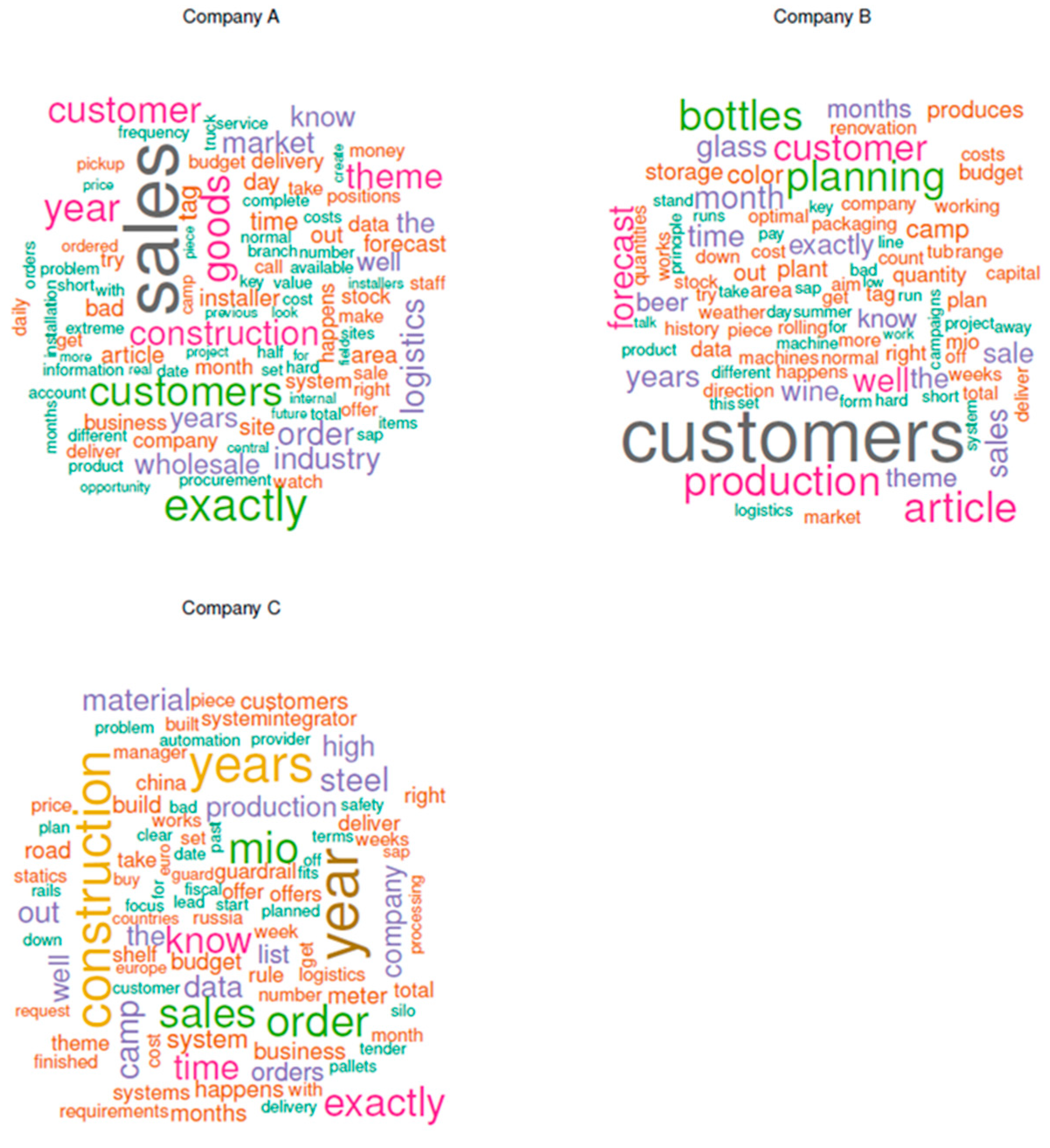
3.1. Word Cloud
To get an overview of the interview contents, we produced word clouds (sometimes also referred to as tag clouds) for each company separately, using the wordcloud package v2.6 [24]. The results are shown in Figure 1. We set the minimum word frequency to 10 and the maximum number of words in each plot to 100. Generating a useful word cloud is a stepwise procedure, since the researchers have to decide on the stop words (i.e., words that do not provide any useful information about the text corpus). Existing lists of such words exist, and the selection is done in an iterative process until a final agreement among the researchers is reached.
Word clouds are a straightforward yet popular tool to visually represent textual data, and their interpretation is straightforward: the bigger a word, the more often it is mentioned throughout the interviews. In our case, it gave the companies a rough idea about the most important topics that emerged during the interviews. Word clouds therefore provide an ideal starting point for further discussions. For instance, the relative size of the words (topics) can be used to critically assess the importance of the respective topic within an organization. Additionally, it is also possible to discover “missing” topics. Figure 1 illustrates which topics are of importance for the respective companies in our sample. Companies A and B seemingly have a strong marketing focus (as is shown by terms such as “customer” or “sales”), while company C concentrates on production and project management (“construction,” “year”).
3.2. Sentiment Analysis
Sentiment analysis is the process of extracting an author’s emotional intent from the text with the goal of determining the general attitude. In the early days of natural language processing (NLP), people used word lists that contained positive words (with valence 1) and negative words (with valence −1). In other words, the valence score rates the polarity of a specific word. Then, either for each sentence or the entire document, they computed a simple polarity score wherein polarity = (number of positive words + number of negative words)/total number of words. More modern approaches, as implemented in the qdap package that we used, incorporate valence shifters (negation and amplifier words), leading to the following sentiment scoring workflow:
- The polarity function scans for positive and negative words within a subjectivity lexicon.
- Once a polarity word is found, the function creates a cluster of terms, including the four preceding and the two following words.
- Within each cluster, the polarity function looks for valence shifters, which give a weight to the polar word (amplifiers add 0.8, negators subtract 0.8). Words with positive polarity are counted as 1, whereas words with negative polarity are counted as −1.
- The grand total of positive, negative, amplifying, and negating words is then divided by the square root of all words in the respective passage. This helps to measure the density of key words.
In our study, we calculated a polarity score for each sentence, which was then averaged (i.e., weighted by the sentence length) in order to get an overall text polarity for each interview. The sentiment analysis enabled us to identify and extract subjective information pertaining to the managers’ responses. We were especially interested in the polarity of each interview based on words that are classified as positive, neutral, or negative. The polarity score is dependent on the dictionary used. In our study, we applied the polarity dictionary by Hu and Liu [25] as implemented in the qdapDictionaries package [26]. This dictionary consists of a list of 6779 words with assigned values of either 1 (positive valence) or −1 (negative valence). Examples for words with positive valence are helpful, enjoyable, enthusiasm, smiling, stimulating. Examples for words with negative valence are unemployed, noise, incomprehensible, upsetting, procrastinate. For this study, we computed the polarity score on a document (i.e., interview) level, but the analysis would have also been possible on a sentence level.
The individual interview polarity scores are shown in Table 1. The average sentiment scores at a company level are 0.40 for Company A, 0.14 for Company B, and 0.43 for Company C. Table 1 also illustrates the wide range of opinions within the specific companies. In company C, for example, the range of sentiment is between −0.58 and 0.65, whereas in company C, almost all interviews are in the positive range, except for one slightly negative one with a score of −0.04. Importantly, it has to be pointed out that the sentiment score heavily depends on the topics being discussed (e.g., exciting new growth strategy vs. problematic project failure). As a starting point, however, it allows for a general assessment of an interviewee’s attitude toward a specific discussion topic expressed in one single score.
3.3. Topic Modeling
Topic modeling is an approach to identify clusters (i.e., topics) within documents. The most popular algorithm for topic modeling is the latent Dirichlet allocation (LDA). For a fixed number of topics (as specified by the researcher), the algorithm associates words as well as interviews with these topics. This happens in a probabilistic way such that each word gets a probability for belonging to each topic, and each interview is assigned a probability for belonging to a specific topic. For algorithmic details on how these probabilities are computed, we refer to the more technical literature such as Grün and Hornik [27]. Based on these resulting posterior probabilities, we were able to extract the most important words that constitute a topic. In Table 2, Table 3 and Table 4, we present the 10 most important words for each company separately. As mentioned, the number of topics needed to be fixed a priori. In practice, researchers run the algorithm for different numbers of topics and use the BIC (Bayesian information criterion) as a statistical measure that helps them to determine a suitable number in addition to subjective interpretability. In our analysis, this strategy resulted in five distinct topics.
Our analyses were based on a document-term matrix (DTM). A DTM is a frequency table with the documents (in our case the interviews) in the rows and the terms (i.e., the words used in the interviews) in the columns. We computed a DTM for each company separately. DTMs are typically large and very sparse (i.e., they have lots of zero entries). Our study revealed the following DTMs:
- Company A: 2929 terms (sparsity of 77%)
- Company B: 2158 terms (sparsity of 71%)
- Company C: 2592 terms (sparsity of 68%)
We then reduced the complexity of the DTMs by considering the most frequently used words only. In order to do so, one can set a raw frequency cutpoint or, a bit more sophisticated, use the “term frequency-inverse document frequency” (tf-idf) to keep relatively frequent words in reflection of how important that word is to a document [28]. According to Kwartler [29], the tf-idf differs from simple term frequency in that it “increases with the term occurrence but is offset by the overall frequency of the word in the corpus” (p. 100).
For the topic models, we decided to use a tf-idf median cut. For computational and interpretation reasons, we cut the number of words in half using a median tf-idf cut and kept only the 50% of most important words, which reduced Company A’s DTM to 1537 columns, Company B’s DTM to 1114 columns, and Company C’s DTM to 1453 columns.
Next, we extracted clusters of words, which are also called topics. We used the LDA [30] to perform the computation. LDA is a generative statistical model and is the most popular approach for computing topic models. It is implemented in the topicmodels package [27]. For each company, we computed the five most important topics and showed the top 10 words that belong to each topic. The results are given in Table 2, Table 3 and Table 4.
The results highlight how topics are composed of specific words and how the various topics differ between companies. In our research project, which focused on supply chain forecasting, it was especially interesting to see which topics were related to the forecasting process within the companies. Similar to word clouds, such topics can be used as a starting point for further discussion, but they also allow for additional insight into what the pending issues within organizations actually are. Topic 1 for company A is apparently about organizing tours for delivering products with trucks and forecasting the respective demand. Topic 2 for company A seems to be also about forecasting and planning, but the occurrence of an unexpected term such as “laughs” might provide an interesting avenue to further follow up and to clarify whether this is meant in a positive or negative way. The interpretation of a particular topic can thus provide a valuable starting point for further discussions with the companies, since it might help to uncover potentially important issues that might otherwise go unnoticed. In topic 1, for example, the term “stock” is also shown, which might indicate potential problems with the provision of supplies (e.g., overstocking or understocking).
3.4. Correspondence Analysis
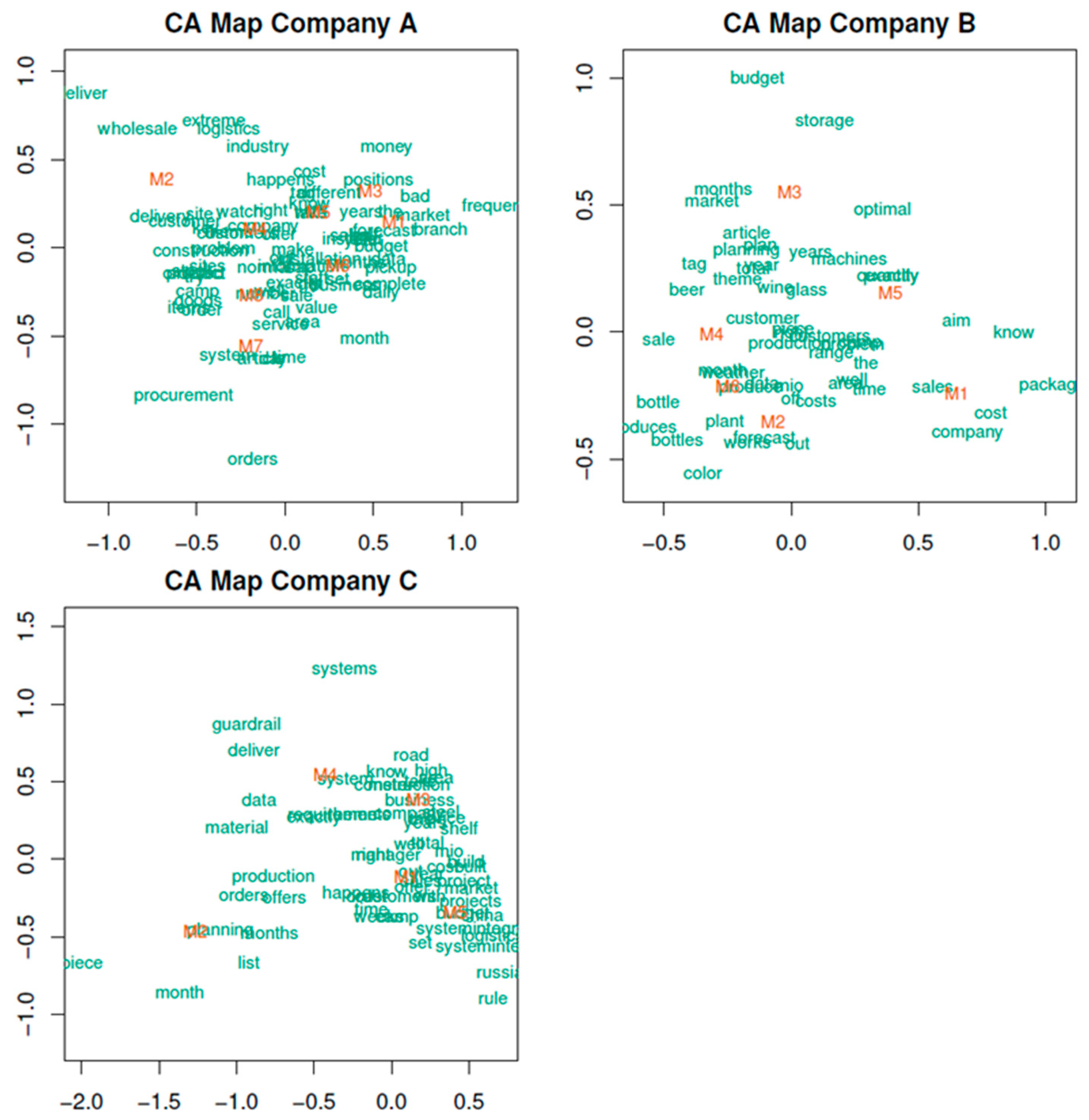
Correspondence analysis (CA) is a technique that is used to scale the row and column categories of a frequency table. In our application, this frequency table is the DTM with the interviews as row categories and the words as column categories. The computation of these scores is based on a singular value decomposition (SVD) for a given dimensionality. After some normalizations of the SVD output (see Mair (2018) [23] for more technical details), the resulting category scores can be plotted, which is usually done in 2D or 3D. Correspondence analysis (CA) simultaneously shows associations among words and managers [31,32].
We applied CA for each company separately and used a simple frequency cutoff for the words. In order to avoid cluttering the resulting CA maps, we used the 20 most frequent words from the respective interviews. For each company, we employed a two-dimensional solution using the anacor package [33] and produced the symmetric CA maps shown in Figure 2. The within-rows distances and the within-column distances correspond to χ2-distances. Mx stands for the respective manager, and the distance to the topics shows the extent to which they “correspond” with those themes. Similar to a principal component analysis or (exploratory) factor analysis [34], a correspondence analysis is a useful multivariate graphical technique for exploratory research. It helps to detect relationships among categorical variables. In our study, the positioning of the managers allows for an easy identification of different work priorities. For example, in company A, manager M1 is in close proximity to terms such as “market,” “years,” “forecast,” and “budget,” indicating that (s)he is involved in planning and scheduling. The term “bad,” which is closely above M1, implies potential problems, which might warrant further investigation. Additionally, the distances between the respective managers and even the words might offer some useful insights. In company C, for example, M2 is distant from the other managers, indicating that (s)he has different tasks and/or preferences as compared to the other ones. In company B, one can see that the terms “budget” and “storage” on the top are distant from the rest of the terms but that they are in relative proximity. This might be a first indicator that the storage in this company either takes up a significant part of the budget or needs to better budgeted. Again, further insight can only be gained by following up with the company, but the CA illustrates that in this specific company storage is apparently a topic that is closely linked to budgeting.
3.5. Multidimensional Scaling
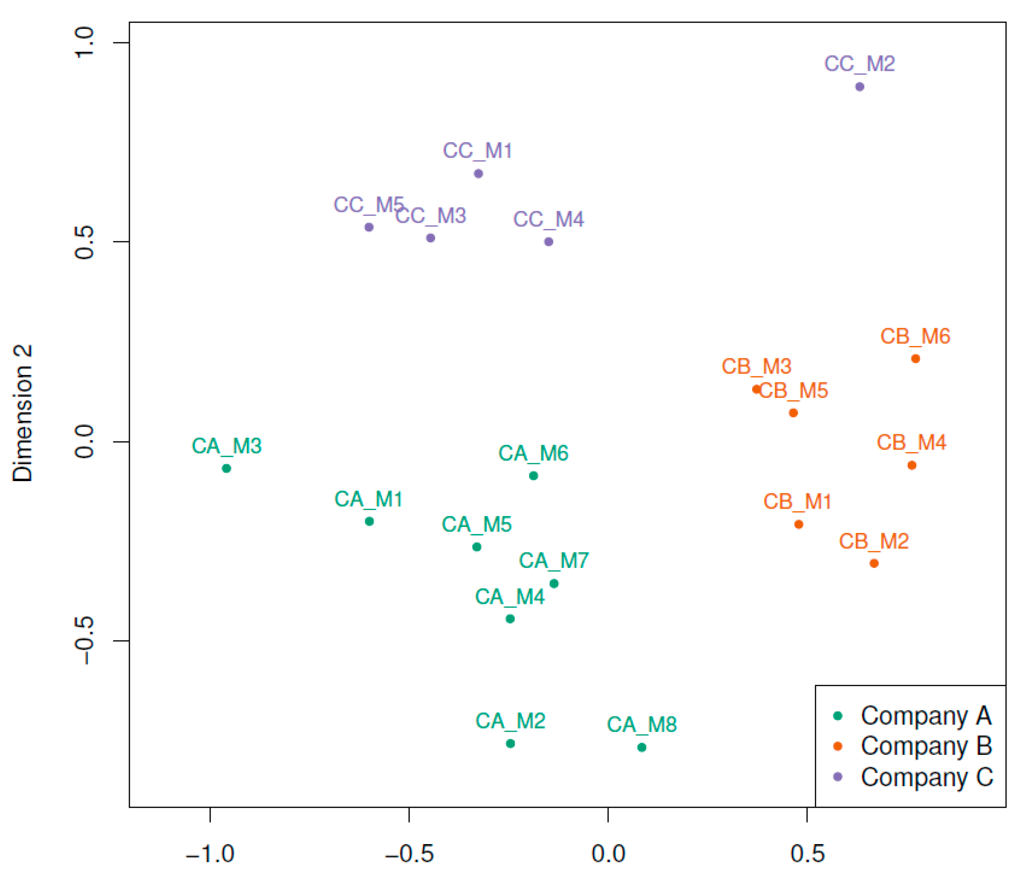
The last method in our analysis is multidimensional scaling (MDS) [35,36] and a subsequent hierarchical cluster analysis. MDS aims to represent input proximities (typically dissimilarities) between objects by means of fitted distances in a low-dimensional space. It therefore visualizes the level of (dis)similarity of cases in a dataset.
For this analysis, we merged all the interviews into a single text corpus and strived to represent similarities between managers. The starting point is again a DTM with 19 rows (i.e., the total number of interviews) and 5059 columns reflecting all the words used in the interviews minus the ones eliminated through data preparation. The first step was to choose a proper dissimilarity measure, which was applied across columns since we are interested in scaling the managers. We picked the cosine distance, which is popular in text mining applications (see e.g. [37]) since it normalizes for document length. The resulting 19 × 19 matrix acts as an input for the MDS computation.
The MDS approach we used is called SMACOF, and it is implemented in the package of the same name [38,39]. SMACOF is a numerical algorithm that solves a target function called “stress.” In simple words, stress incorporates the observed dissimilarities and the fitted dissimilarities. The difference between the two should be as small as possible and hence the stress function is minimized. The smaller the resulting stress value, the better the solution. In order to achieve a small stress value, SMACOF provides the option to include an additional transformation step on the observed dissimilarities. For instance, in our application, we performed an ordinal transformation leading to a stress-1 value of 0.175. Stress-1 is a simple normalization of the raw stress value such that it becomes scale-free. Similar to CA, we aimed to fit a 2D or 3D solution as the configuration plot is the main output of MDS and is subject to interpretation. The configuration essentially represents a map of the objects that can be interpreted in a very intuitive way. The closer two points are in the configuration, the more similar they are. In our application, these points represent the interviews for all three companies. Figure 3 shows the resulting configuration plot, and we see that MDS neatly reveals three clusters of managers, according to the company they work for. This result indicates that the managers belonging to one company are more similar to each other when it comes to the topics they deal with (or their choice of words) as opposed to managers from other companies. This can potentially be traced back to the varying working areas, but could also be a strong indicator for differing organizational cultures that impact the choice of words and the respective way in which they see things. Interestingly, M2 from company C on the upper right seems to be an outlier, which might warrant further attention to clarify why his/her choice of words is so different from the other managers.
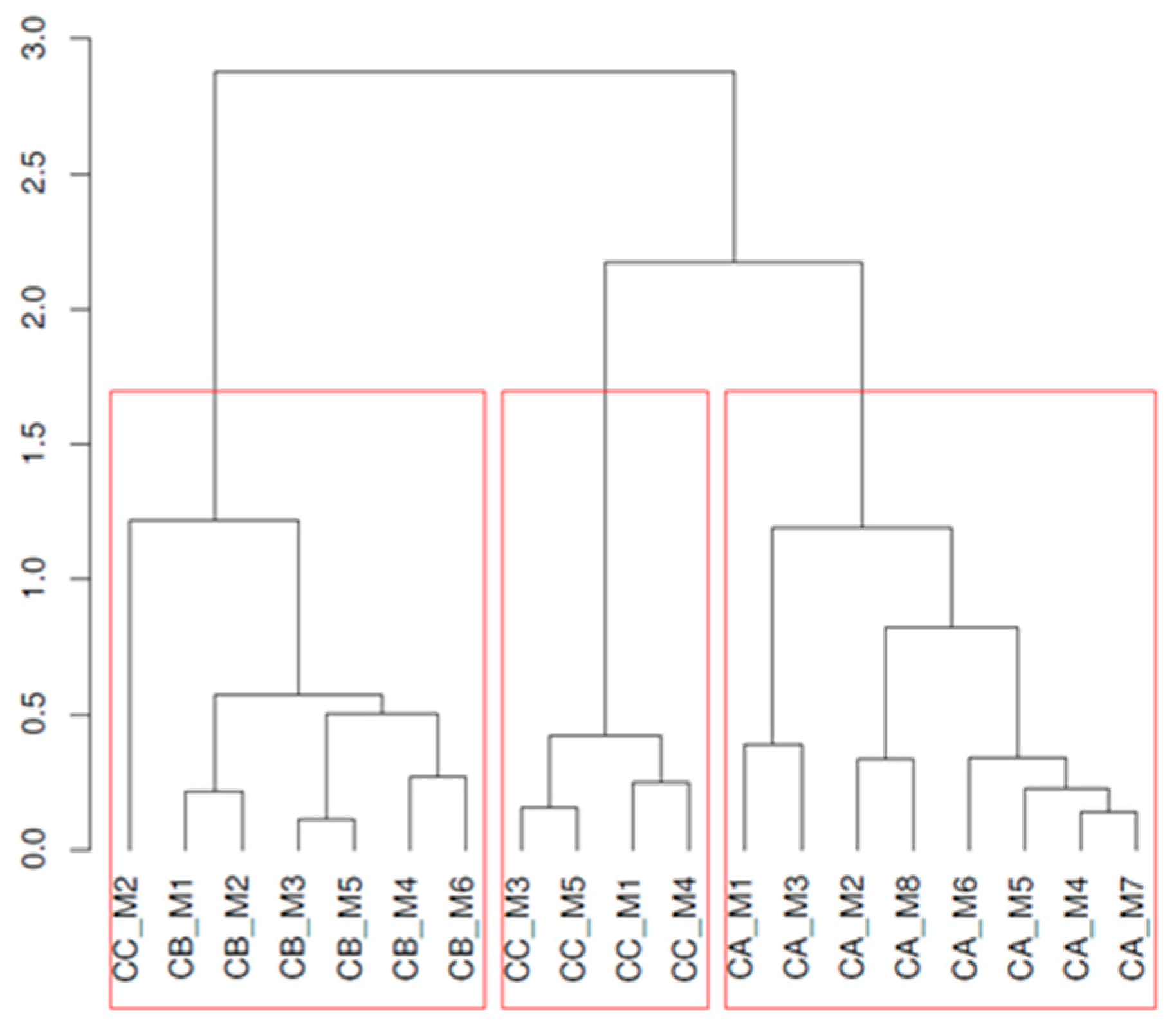
This clear cluster separation based on the words used in the interviews is confirmed by a hierarchical cluster analysis based on the fitted MDS distance matrix. By cutting the dendrogram (see Figure 4), based on Ward clustering at a value corresponding to 3 clusters (since we have 3 companies), we see that the resulting clusters perfectly separate the managers from each other. In this example, the clusters represent the companies they are working for. This is also an indicator of the coherence of the respective topics within and between the companies.
4. Conclusions and Further Research
In this paper, we discuss five techniques for automated text analysis that are underrepresented in logistics and supply chain management research. We believe, however, that they offer a huge potential for identifying patterns buried in large chunks of textual data and, if used in an exploratory manner, might even reveal interesting avenues for future research. We present the results of an empirical research project on supply chain forecasting to exemplify how different text analysis techniques can be applied and interpreted appropriately. Our presentation of the findings of the five techniques will give other researchers an understanding about what kind of information they can uncover when it comes to the interpretation of qualitative textual data.
Of course, the same procedures can be applied to all kinds of textual data, which might be of interest for logistics and supply chain researchers (e.g., reports, information on websites, or external media coverage) and can help them to detect important emerging trends [40,41]. It is up to the researchers’ creativity to find topics that are important for logistics and supply chain management and to interpret the extracted information accordingly.
Apart from applying existing, albeit state-of-the-art procedures of text analysis, this study is also highly explorative. By using automated text analysis, data can be analyzed in a fast and impartial way that does not depend on human judgement. Specifically, we applied the following techniques:
- Word clouds: Our analysis shows which topics (words) were most frequently mentioned. This allows managers and researchers to identify core topics in textual data.
- Sentiment analysis: We computed polarity scores based on managers’ sentiments. In our example, we were especially interested whether the average polarity scores differ across companies. The results illustrate how sentiment analysis can be used to uncover the emotional level of textual data, which reveals how certain topics are perceived in general.
- Topic models: Using the document-term matrix as a starting point, we clustered the texts based on dominating topics by means of LDA. Each resulting cluster contains topics ordered in relation to their importance. This analysis reveals topics that exist within a specific company (or document) and also allows for an easy comparison of what is important between different companies (or documents).
- Correspondence analysis: We computed associations between the words being used and the respective managers. A visual representation allows for an easy interpretation of how managers and topics are related. This helps to detect which interests and priorities a specific manager has and can easily be extended to reveal any kind of relationship between and within two groups of variables.
- Multidimensional scaling (MDS): We were interested in representing similarities between the interviews. Clusters of managers emerged that highlight the differences between companies and revealed underlying dimensions. This technique is frequently used in marketing research (e.g., for market segmentation, product positioning, brand image measurement, and brand similarity studies) but, as we have shown in our study, it might be equally useful to position respondents from other functional areas according to their respective preferences and perceptions.
The application of text analysis is by no means limited to the techniques shown in this paper. Amongst others, further options include a dynamic sentiment analysis to identify changes in sentiments over time and a readability analysis, which indicates the ease with which readers can actually understand written texts. In light of the many qualitative studies conducted in logistics and supply chain management research, be it literature reviews, case studies, or, as shown in this paper, expert interviews, we suggest that researchers add automated text mining techniques to their existing portfolio of research methods in order to be able to make the most out of the qualitative data they have at their disposal.
Author Contributions
Conceptualization, H.T. and P.M.; methodology, P.M.; software, P.M.; validation, H.T.; formal analysis, P.M.; investigation, H.T.; writing—original draft preparation, H.T and P.M.; writing—review and editing, P.M. and H.T.; visualization, P.M.; project administration, H.T.; funding acquisition, H.T. All authors have read and agreed to the published version of the manuscript.
Funding
This research received no external funding.
Conflicts of Interest
The authors declare no conflict of interest.
Appendix A. R Source Code
## ----------------------- Installing the required packages -----------------
if (!require("wordcloud")) {install.packages("wordcloud"); library("wordcloud")}
if (!require("smacof")) {install.packages("smacof"); library("smacof")}
if (!require("anacor")) {install.packages("anacor"); library("anacor")}
if (!require("tm")) {install.packages("tm"); library("tm")}
if (!require("slam")) {install.packages("slam"); library("slam")}
if (!require("qdap")) {install.packages("qdap"); library("qdap")}
if (!require("koRpus")) {install.packages("koRpus"); library("koRpus")}
if (!require("topicmodels")) {install.packages("topicmodels"); library("topicmodels")}
if (!require("translateR")) {install.packages("translateR"); library("translateR")}
require("lattice")
## ---------------------- load data ----------------------------------
load("c1Corp.rda") ## Company 1 answer corpus (8 interviews/documents)
load("c2Corp.rda") ## Company 2 answer corpus (6 interviews/documents)
load("c3Corp.rda") ## Company 3 answer corpus (5 interviews/documents)
c1Corp_punct <- c1Corp ## with punctuation
c1Corp <- tm_map(c1Corp, removePunctuation, preserve_intra_word_dashes = TRUE) ## without punctuation
c2Corp_punct <- c2Corp ## with punctuation
c2Corp <- tm_map(c2Corp, removePunctuation, preserve_intra_word_dashes = TRUE) ## without punctuation
c3Corp_punct <- c3Corp ## with punctuation
c3Corp <- tm_map(c3Corp, removePunctuation, preserve_intra_word_dashes = TRUE) ## without punctuation
## ---------------------- Word Clouds -----------------------------
## wordclouds for each company
set.seed(666)
x11()
wordcloud(c1Corp, colors = brewer.pal(8, "Dark2"), min.freq = 10) ## C1
wordcloud(c2Corp, colors = brewer.pal(8, "Dark2"), min.freq = 10) ## C2
wordcloud(c3Corp, colors = brewer.pal(8, "Dark2"), min.freq = 10) ## C3
## ---------------------- Sentiment Analysis ----------------------
## We us3 the German Sentiment Wortschatz SentiWS
## http://asv.informatik.uni-leipzig.de/download/sentiws.html
temp <- tempfile()
download.file("http://wortschatz.uni-leipzig.de/download/SentiWS_v1.8c.zip", temp)
## the following function organizes all positive and negative words from SentiWS
readAndflattenSentiWS <- function(filename) {
words <- readLines(unz(temp, filename), encoding = "UTF-8")
words <- sub("\\|[A-Z]+\t[0-9.-]+\t?", ",", words)
words <- unlist(strsplit(words, ","))
words <- tolower(words)
return(words)
}
posWords <- readAndflattenSentiWS("SentiWS_v1.8c_Positive.txt") ## positive words
negWords <- readAndflattenSentiWS("SentiWS_v1.8c_Negative.txt") ## negative words
## Simple sentiment analyses for each company separately
## +1 for each positive match, -1 for each negative match (standardized by the number of words used)
## --- Company 1: C1
dtmat_c1 <- DocumentTermMatrix(c1Corp) ## C1 document term matrix
c1Words <- dtmat_c1$dimnames$Terms[dtmat_c1$j] ## all the words from C1
posmatches <- sum(!is.na(match(c1Words, posWords))) ## C1 positive words count
negmatches <- sum(!is.na(match(c1Words, negWords))) ## C1 negative words count
sentscore_c1 <- (posmatches - negmatches)/length(c1Words)
sentscore_c1
## positive sentiment score for C1
## --- Company 2: C2
dtmat_c2 <- DocumentTermMatrix(c2Corp) ## C2 document term matrix
c2Words <- dtmat_c2$dimnames$Terms[dtmat_c2$j] ## all the words from C2
posmatches <- sum(!is.na(match(c2Words, posWords))) ## C2 positive words count
negmatches <- sum(!is.na(match(c2Words, negWords))) ## C2 negative words count
sentscore_c2 <- (posmatches - negmatches)/length(c2Words)
sentscore_c2
## positive sentiment score for C2
## --- Company 3: C3
dtmat_c3 <- DocumentTermMatrix(c3Corp) ## C3 document term matrix
c3Words <- dtmat_c3$dimnames$Terms[dtmat_c3$j] ## all the words from C3
posmatches <- sum(!is.na(match(c3Words, posWords))) ## C3 positive words count
negmatches <- sum(!is.na(match(c3Words, negWords))) ## C3 negative words count
sentscore_c3 <- (posmatches - negmatches)/length(c3Words)
sentscore_c3
## positive sentiment score for C3
## C3 has the highest sentiment score, followed by C1, and then C2.
## -------------------- Correspondence Analysis ----------------------
## Based on the most frequent words we examine how the words are related to each other
## and how the respondents are related to each other
## for each company we select words that were mentioned at least 20 times
## we could do this a bit more sophisticated by using the TFIDF (see topic models below)
wordcut <- 20
## --- C1
dtmat <- as.matrix(dtmat_c1) ## convert into a regular matrix
ind <- which(colSums(dtmat) >= wordcut)
camat <- dtmat[, ind]
## rownames(camat) <- paste0("IP", 1:nrow(camat)) ## anonymous version
rownames(camat) <- c("I1_c1", "I2_c1", "I3_c1", "I4_c1", "I5_c1", "I6_c1", "I7_c1", "I8_c1") #Ix stands for the respective interviewee
ca_c1 <- anacor(camat)
ca_c1
plot(ca_c1, conf = NULL, main = "C1 Configuration")
## --- C2
dtmat <- as.matrix(dtmat_c2)
ind <- which(colSums(dtmat) >= wordcut)
camat <- dtmat[, ind]
## rownames(camat) <- paste0("IP", 1:nrow(camat)) ## anonymous version
rownames(camat) <- c("I2_c2", "I2_c2", "I3_c2", "I4_c2", "I5_c2", "I6_c2")
ca_c2 <- anacor(camat)
ca_c2
plot(ca_c2, conf = NULL, main = "C2 Configuration")
## --- C3
dtmat <- as.matrix(dtmat_c3)
ind <- which(colSums(dtmat) >= wordcut)
camat <- dtmat[, ind]
## rownames(camat) <- paste0("IP", 1:nrow(camat)) ## anonymous version
rownames(camat) <- c("I1_c3", "I2_c3", "I3_c3", "I4_c3", "I5_c3")
ca_c3 <- anacor(camat)
ca_c3
plot(ca_c3, conf = NULL, main = "C3 Configuration")
## ------------- Topic Models: Clustering -----------------------------
## Now let's do some clustering using topic models
## We are using the term frequency-inverse document frequency for keeping frequent words (instead of a raw cut):
## C1
tfidf <- tapply(dtmat_c1$v/row_sums(dtmat_c1)[dtmat_c1$i], dtmat_c1$j, mean) * log2(nDocs(dtmat_c1)/col_sums(dtmat_c1 > 0))
cut <- median(tfidf) ## let's do a median cut
dtm2_c1 <- dtmat_c1[, tfidf >= cut]
ncol(dtm2_c1)
## C2
tfidf <- tapply(dtmat_c2$v/row_sums(dtmat_c2)[dtmat_c2$i], dtmat_c2$j, mean) * log2(nDocs(dtmat_c2)/col_sums(dtmat_c2 > 0))
cut <- median(tfidf) ## let's do a median cut
dtm2_c2 <- dtmat_c2[, tfidf >= cut]
ncol(dtm2_c2)
## C3
tfidf <- tapply(dtmat_c3$v/row_sums(dtmat_c3)[dtmat_c3$i], dtmat_c3$j, mean) * log2(nDocs(dtmat_c3)/col_sums(dtmat_c3 > 0))
cut <- median(tfidf) ## let's do a median cut
dtm2_c3 <- dtmat_c3[, tfidf >= cut]
ncol(dtm2_c3)
## --- clustering
k <- 10 ## number of clusters
SEED <- 666 ## set seed for reproducibility
topmod_c1 <- LDA(dtm2_c1, k = k, control = list(seed = SEED)) ## LDA for C1
topmod_c2 <- LDA(dtm2_c2, k = k, control = list(seed = SEED)) ## LDA for C2
topmod_c3 <- LDA(dtm2_c3, k = k, control = list(seed = SEED)) ## LDA for C3
topterms_c1 <- terms(topmod_c1, 10) ## 10 clusters, top 10 words
topterms_c1 ## C1 topics
topterms_c2 <- terms(topmod_c2, 10) ## 10 clusters, top 10 words
topterms_c2 ## C2 topics
topterms_c3 <- terms(topmod_c1, 10) ## 10 clusters, top 10 words
topterms_c3 ## C3 topics
## ------------------- Multidimensional Scaling: Similarity of Interviews -------
allCorp <- c(c1Corp, c2Corp, c3Corp) ## merge all interviews into a single corpus
tdm <- TermDocumentMatrix(allCorp) ## full document term matrix
dim(tdm)
cosine_dist_mat <- 1 - crossprod_simple_triplet_matrix(tdm)/(sqrt(col_sums(tdm^2) %*% t(col_sums(tdm^2)))) ## cosine distances
dim(cosine_dist_mat)
rownames(cosine_dist_mat) <- c("I1_c1", "I2_c1", "I3_c1", "I4_c1", "I5_c1", "I6_c1", "I7_c1", "I8_c1",
"I1_c2", "I2_c2", "I3_c2", "I4_c2", "I5_c2", "I6_c2",
"I1_c3", "I2_c3", "I3_c3", "I4_c3", "I5_c3")
fitmds <- mds(cosine_dist_mat, type = "ordinal") ## fit 2D ordinal MDS
fitmds
plot(fitmds, plot.type = "Shepard") ## check goodness-of-fit: OK
colvec <- c(rep(1, 8), rep(2, 6), rep(4, 5))
x11()
plot(fitmds, label.conf = list(col = colvec), col = colvec)
legend("bottomleft", legend = c("C1", "C2", "C3"), pch = 20, col = c(1,2,4))
## That's an interesting picture: the companies are nicely separated in the MDS
## hierarchical clustering:
fitclust <- hclust(as.dist(cosine_dist_mat), method = "ward.D2")
x11()
plot(fitclust, hang = -1, ann = FALSE)
title("Interviews Dendrogram")
rect.hclust(fitclust, k = 3)
## this confirms what we have seen in MDS
cutree(fitclust, k = 3) ## 3 cluster membership
References
- Ghadge, A.; Dani, S.; Kalawsky, R. Supply chain risk management: Present and future scope. Int. J. Logist. Manag. 2012, 23, 313–339. [Google Scholar] [CrossRef] [Green Version]
- Pournader, M.; Kach, A.; Talluri, S. A Review of the Existing and Emerging Topics in the Supply Chain Risk Management Literature. Decis. Sci. 2020, 51, 867–919. [Google Scholar] [CrossRef]
- Ma, K.; Pal, R.; Gustafsson, E. What modelling research on supply chain collaboration informs us? Identifying key themes and future directions through a literature review. Int. J. Prod. Res. 2019, 57, 2203–2225. [Google Scholar] [CrossRef] [Green Version]
- Rozemeijer, F.; Quintens, L.; Wetzels, M.; Gelderman, C. Vision 20/20: Preparing today for tomorrow’s challenges. J. Purch. Supply Manag. 2012, 18, 63–67. [Google Scholar] [CrossRef]
- Cecere, L. A Practitioner’s Guide to Demand Planning. Supply Chain Manag. Rev. 2013, 17, 40–46. [Google Scholar]
- Shah, S.; Lütjen, M.; Freitag, M. Text Mining for Supply Chain Risk Management in the Apparel Industry. Appl. Sci. 2021, 11, 2323. [Google Scholar] [CrossRef]
- Folinas, D.; Tsolakis, N.; Aidonis, D. Logistics Services Sector and Economic Recession in Greece: Challenges and Opportunities. Logistics 2018, 2, 16. [Google Scholar] [CrossRef] [Green Version]
- Rossetti, C.L.; Handfield, R.; Dooley, K.J. Forces, trends, and decisions in pharmaceutical supply chain management. Int. J. Phys. Distrib. Logist. Manag. 2011, 41, 601–622. [Google Scholar] [CrossRef]
- Abrahams, A.; Fan, W.; Wang, A.; Zhang, Z.; Jiao, J. An Integrated Text Analytic Framework for Product Defect Discovery. Prod. Oper. Manag. 2015, 24, 975–990. [Google Scholar] [CrossRef]
- Alfaro, C.; Cano-Montero, J.; Gómez, J.; Moguerza, J.M.; Ortega, F. A multi-stage method for content classification and opinion mining on weblog comments. Ann. Oper. Res. 2016, 236, 197–213. [Google Scholar] [CrossRef]
- Näslund, D. Logistics needs qualitative research—Especially action research. Int. J. Phys. Distrib. Logist. Manag. 2002, 32, 321–338. [Google Scholar] [CrossRef]
- Hussein, M.; Eltoukhy, A.E.; Karam, A.; Shaban, I.A.; Zayed, T. Modelling in off-site construction supply chain management: A review and future directions for sustainable modular integrated construction. J. Clean. Prod. 2021, 310, 127503. [Google Scholar] [CrossRef]
- Treiblmaier, H.; Mair, P. Applying Text Mining in Supply Chain Forecasting: New Insights through Innovative Approaches. In Proceedings of the 23rd EurOMA Conference, Trondheim, Norway, 17–22 June 2016. [Google Scholar]
- Treiblmaier, H. A Framework for Supply Chain Forecasting Literature. Acta Tech. Corviniensis Bull. Eng. 2015, 7, 49–52. [Google Scholar]
- Nitsche, B. Unravelling the Complexity of Supply Chain Volatility Management. Logistics 2018, 2, 14. [Google Scholar] [CrossRef] [Green Version]
- Subramanian, L. Effective Demand Forecasting in Health Supply Chains: Emerging Trend, Enablers, and Blockers. Logistics. 2021, 5, 12. [Google Scholar] [CrossRef]
- Treiblmaier, H. Optimal levels of (de)centralization for resilient supply chains. Int. J. Logist. Manag. 2018, 29, 435–455. [Google Scholar] [CrossRef]
- Ehrenhuber, I.; Treiblmaier, H.; Engelhardt-Nowitzki, C.; Gerschberger, M. Toward a framework for supply chain resilience. Int. J. Supply Chain Oper. Resil. 2015, 1, 339. [Google Scholar] [CrossRef]
- R Core Team. R: The R Project for Statistical Computing; R Foundation for Statistical Computing: Vienna, Austria, 2021. [Google Scholar]
- Rinker, T.W. Qdap: Quantitative Discourse Analysis Package. In R Package Version 2.2.4; 2015; Available online: https://github.com/trinker/qdap (accessed on 12 July 2021).
- Feinerer, I.; Hornik, K.; Meyer, D. Text Mining Infrastructure in R. J. Stat. Softw. 2008, 25, 1–54. [Google Scholar] [CrossRef] [Green Version]
- Lucas, C.; Tingley, D. TranslateR: Bindings for the Google and Microsoft Translation. In R Package Version 1.0; 2014; Available online: https://rdrr.io/github/ChristopherLucas/translateR/ (accessed on 15 July 2021).
- Mair, P. Modern Psychometrics with R; Use R! Springer International Publishing: Basel, Switzerland, 2018; ISBN 978-3-319-93175-3. [Google Scholar]
- Fellows, I. Wordcloud: Word Clouds. Available online: https://CRAN.R-project.org/package=wordcloud (accessed on 27 May 2021).
- Hu, M.; Liu, B. Mining Opinion Features in Customer Reviews. In Proceedings of the National Conference on Artificial Intelligence (AAAI), San Jose, CA, USA, 25–29 July 2004; Volume 4, pp. 755–760. [Google Scholar]
- Rinker, T.W. QdapDictionaries: Dictionaries to Accompany the Qdap Package 1.0.7; University at Buffalo: Buffalo, NY, USA, 2013. [Google Scholar]
- Grün, B.; Hornik, K. Topicmodels: An R Package for Fitting Topic Models. J. Stat. Softw. 2011, 40, 313–339. [Google Scholar] [CrossRef] [Green Version]
- Blei, D.M.; Lafferty, J.D. Topic Models. In Text Mining: Classification, Clustering, and Applications; Srinivasta, A., Sahami, M., Eds.; Chapman & Hall: New York, NY, USA, 2009; CRC Press: New York, NY, USA; pp. 71–93. [Google Scholar]
- Kwartler, T. Text Mining in Practice with R|Wiley; John Wiley & Sons: New York, NY, USA, 2017; ISBN 978-1-119-28201-3. [Google Scholar]
- Blei, D.M.; Ng, A.Y.; Jordan, M.I. Latent Dirichlet Allocation. J. Mach. Learn. Res. 2003, 3, 993–1022. [Google Scholar]
- Greenacre, M. Correspondence Analysis in Practice; Chapman and Hall: New York, NY, USA; CRC: New York, NY, USA, 2017; ISBN 978-1-315-36998-3. [Google Scholar]
- Bécue-Bertaut, M. Textual Data Science with R; CRC Press: Boca Raton, FL, USA, 2021. [Google Scholar]
- De Leeuw, J.; Mair, P. Simple and Canonical Correspondence Analysis Using the R Package anacor. J. Stat. Softw. 2009, 31, 1–18. [Google Scholar] [CrossRef] [Green Version]
- Treiblmaier, H.; Filzmoser, P. Exploratory factor analysis revisited: How robust methods support the detection of hidden multivariate data structures in IS research. Inf. Manag. 2010, 47, 197–207. [Google Scholar] [CrossRef]
- Borg, I.; Groenen, P.J.F. Modern Multidimensional Scaling: Theory and Applications, 2nd ed.; Springer Series in Statistics; Springer: New York, NY, USA, 2005; ISBN 978-0-387-25150-9. [Google Scholar]
- Borg, I.; Groenen, P.J.F.; Mair, P. Applied Multidimensional Scaling and Unfolding, 2nd ed.; Springer Briefs in Statistics; Springer International Publishing: Basel, Switzerland, 2018; ISBN 978-3-319-73470-5. [Google Scholar]
- Chen, Y.; Garcia, E.K.; Gupta, M.R.; Rahimi, A.; Cazzanti, L. Similarity-Based Classification: Concepts and Algorithms. J. Mach. Learn. Res. 2009, 10, 747–776. [Google Scholar]
- de Leeuw, J.; Mair, P. Multidimensional Scaling Using Majorization: SMACOF in R. J. Stat. Softw. 2009, 31, 1–30. [Google Scholar] [CrossRef] [Green Version]
- Mair, P.; Groenen, P.J.F.; De Leeuw, J. More on Multidimensional Scaling and Unfolding in R: Smacof Version 2. J. Stat. Softw. 2021. Available online: https://cran.r-project.org/web/packages/smacof/vignettes/smacof.pdf (accessed on 15 July 2021).
- Treiblmaier, H. Combining Blockchain Technology and the Physical Internet to Achieve Triple Bottom Line Sustainability: A Comprehensive Research Agenda for Modern Logistics and Supply Chain Management. Logistics 2019, 3, 10. [Google Scholar] [CrossRef] [Green Version]
- Rejeb, A.; Keogh, J.G.; Simske, S.J.; Stafford, T.; Treiblmaier, H. Potentials of blockchain technologies for supply chain collaboration: A conceptual framework. Int. J. Logist. Manag. 2021, 32, 973–994. [Google Scholar] [CrossRef]
Figure 1.
Word clouds for companies A, B, and C.

Figure 2.
Symmetric CA maps for companies A, B, and C.

Figure 3.
MDS configurations on full dataset.

Figure 4.
Dendrogram Ward clustering on MDS distances (3-cluster solution).


Table 1.
Interview Sentiment Scores.
| Company A | Company B | Company C | |
|---|---|---|---|
| 1 | 0.49 | 0.33 | 0.20 |
| 2 | 0.65 | 0.06 | −0.04 |
| 3 | −0.17 | 0.65 | 1.25 |
| 4 | −0.30 | −0.58 | 0.08 |
| 5 | 0.82 | −0.06 | 0.68 |
| 6 | 0.46 | 0.45 | |
| 7 | 0.99 | ||
| 8 | 0.22 | ||
| avg | 0.40 | 0.14 | 0.43 |
Table 2.
Topics Company A.
| Topic 1 | Topic 2 | Topic 3 | Topic 4 | Topic 5 | |
|---|---|---|---|---|---|
| 1 | logistics | data | time | frequency | logistics |
| 2 | forecast | system | orders | branch | deliver |
| 3 | positions | forecast | business | pickup | stock |
| 4 | term | time | procurement | business | truck |
| 5 | tours | product | stock | channels | extreme |
| 6 | stock | business | items | forecast | logistic |
| 7 | leave | laughs | ordered | data | ordered |
| 8 | talks | volume | account | positions | distribution |
| 9 | thing | development | internal | quality | major |
| 10 | truck | evaluate | professional | extrapolation | sale |
Table 3.
Topics Company B.
| Topic 1 | Topic 2 | Topic 3 | Topic 4 | Topic 5 | |
|---|---|---|---|---|---|
| 1 | budget | overdue | bottle | mio | bottle |
| 2 | stand | forecast precision | count | effect | march |
| 3 | market | days | million | affected | mio |
| 4 | board | form | deviation | danger | rolling |
| 5 | budgeting | moment | takes | quarter | giant |
| 6 | contract | past | pcs | advantage | classic |
| 7 | directors | campaign | budget | carton | increases |
| 8 | rolling | claims | case | controlling | middle |
| 9 | theoretical | figure | hand | goods | rebuilt |
| 10 | contracts | any | larger | input | drip |
Table 4.
Topics Company C.
| Topic 1 | Topic 2 | Topic 3 | Topic 4 | Topic 5 | |
|---|---|---|---|---|---|
| 1 | logistics | data | time | frequency | logistics |
| 2 | forecast | system | orders | branch | deliver |
| 3 | positions | forecast | business | pickup | stock |
| 4 | term | time | procurement | business | truck |
| 5 | tours | product | stock | channels | extreme |
| 6 | stock | business | items | forecast | logistic |
| 7 | leave | laughs | ordered | data | ordered |
| 8 | talks | volume | account | positions | distribution |
| 9 | thing | development | internal | quality | major |
| 10 | truck | evaluate | professional | extrapolation | sale |
Publisher’s Note: MDPI stays neutral with regard to jurisdictional claims in published maps and institutional affiliations. |
© 2021 by the authors. Licensee MDPI, Basel, Switzerland. This article is an open access article distributed under the terms and conditions of the Creative Commons Attribution (CC BY) license (https://creativecommons.org/licenses/by/4.0/).
Share and Cite
MDPI and ACS Style
Treiblmaier, H.; Mair, P. Textual Data Science for Logistics and Supply Chain Management. Logistics 2021, 5, 56. https://0-doi-org.brum.beds.ac.uk/10.3390/logistics5030056
AMA Style
Treiblmaier H, Mair P. Textual Data Science for Logistics and Supply Chain Management. Logistics. 2021; 5(3):56. https://0-doi-org.brum.beds.ac.uk/10.3390/logistics5030056
Chicago/Turabian StyleTreiblmaier, Horst, and Patrick Mair. 2021. "Textual Data Science for Logistics and Supply Chain Management" Logistics 5, no. 3: 56. https://0-doi-org.brum.beds.ac.uk/10.3390/logistics5030056