Article

Adaptive Mesh Refinement Strategies for Cost-Effective Eddy-Resolving Transient Simulations of Spray Dryers

by
Jairo Andrés Gutiérrez Suárez
1,*,†,
Carlos Humberto Galeano Urueña
2,† and
Alexánder Gómez Mejía
1,†
1
Grupo de Investigación en Biomasa y Optimización Térmica de Procesos, Departamento de Ingeniería Mecánica y Mecatrónica, Facultad de Ingeniería, Universidad Nacional de Colombia—Sede Bogotá, Cra 45 #26-85, Bogotá 111321, Colombia
2
Grupo de Modelado y Métodos Numéricos en Ingeniería, Departamento de Ingeniería Mecánica y Mecatrónica, Facultad de Ingeniería, Universidad Nacional de Colombia—Sede Bogotá, Cra 45 #26-85, Bogotá 111321, Colombia
*
Author to whom correspondence should be addressed.
These authors contributed equally to this work.
Submission received: 29 August 2023 / Revised: 27 September 2023 / Accepted: 6 October 2023 / Published: 18 October 2023
(This article belongs to the Special Issue Feature Papers in Chemical Engineering)

Abstract

:
The use of adaptive meshing strategies to perform cost-effective transient simulations of spray drying processes is evaluated. These simulations are often computationally expensive, given the large differences between the characteristic times of the central jet and those of the unsteady flow developed at its periphery. Managing the computational cost through the control of the grid resolution by regions is inadequate in many of these applications since the grid resolution requirements change dynamically within the domain. These conditions are related to the unsteady nature of the flow in both the central jet and the flow recirculation zones. Therefore, the application of adaptive mesh refinement (AMR) strategies is recommended. In this paper, general AMR criteria based on relative errors are evaluated by testing three mesh adaptation criteria: velocity gradient, pressure gradient, and vorticity. This evaluation is performed using a low-cost turbulence model with eddy resolution (DDES) in two different types of drying chambers, in which experimental measurements are available. The use of AMR exerts appreciable effects on decreasing computational costs and contributes to the capture of large eddies in critical regions. The present approach provides an appropriate balance between solution accuracy and computational cost. By using a correct AMR configuration, it is possible to obtain results similar to those obtained on a fixed grid but reducing the computational costs by 3 to 5 times.

Graphical Abstract

1. Introduction

Spray drying represents a well-known example of particle-laden flow where a hot-gas jet interacts with a spray cloud to produce high-quality powders. General aspects of spray drying processes are well documented in the literature, e.g., Santos et al. [1]. The interaction between the gas and liquid phases is complex [2] and involves several thermo-physical processes affecting the properties of the powder [3]. These processes are strongly related to the gas-flow dynamics inside the drying chamber [4], and its modeling is essential to predict the performance of a spray dryer [5]. A large number of previous studies using computational fluid dynamics (CFD) have assumed a steady-state approach to model the airflow inside the drying chamber, such as Woo et al. [6], but the current trend towards using a transient approach is now widely accepted [4]. The assumption of a steady-flow field has been found to be inaccurate, as demonstrated by various experimental and CFD studies.
In a pilot-scale spray chamber, Southwell and Langrish [7] used visual techniques, which revealed a swirl-dependent chaotic behavior of the flow in significant portions of the drying chamber. They also visualized a central vortex that exhibited temporal and spatial unsteadiness. Using laser-Doppler anemometry, Southwell and Langrish [8] further investigated the effect of swirl on flow stability. Their findings showed that, for all studied swirl settings (ranging from 0° to 45°) at the inlet, no swirl angle resulted in steady flow behavior within the drying chamber. They also reported the existence of slow, large, and unsteady recirculation regions that altered the flow direction. These flow instabilities are more pronounced in short-form spray dryers [9] with lower swirl values at the inlet jet. Lebarbier et al. [10] employed image analysis techniques (light sheet) to study the flow patterns in a 1/31 scale model of an industrial-sized spray chamber. These observations also revealed a strong time-dependent precessing behavior in the central jet.
Transient CFD studies have also confirmed the time-dependent nature of the airflow. In a CFD study of gas flow inside a pilot-scale spray dryer with and without swirl, Langrish et al. [11] explored the time-dependent nature of flow patterns. In this study, they found that even under zero inlet swirl conditions, the central jet exhibited slight precession around the axis, challenging the validity of the steady-state assumption. In a three-dimension transient study of gas-particle interactions in an industrial-scale spray dryer, Jin and Chen [12] reported low-frequency oscillations of the central jet and three-dimensionality in the flow field, leading to a more realistic dispersion of particles within the chamber. Using a large-eddy simulation approach (LES) to model airflow in a semi-industrial-sized spray chamber, Jongsma et al. [13] reported the existence of large-scale flow structures that exhibited a transient nature, particularly when the central jet was deflected towards the walls. This mechanism is particularly significant for an accurate prediction of the wall deposition of particles.
A further drawback of the steady-state approach is its apparent inability to reach a converged state, a matter debated by Fletcher and Langrish [14] and verified by Lebarbier et al. [10]. This limitation also emerged in preliminary simulations conducted in this study. While some authors have reported residual convergence in steady-state simulations, coarse grids may attenuate these instabilities [9], hence failing to replicate critical flow phenomena within the drying chamber and potentially resulting in misleading results. If sufficient computational resources are available, a transient approach within a three-dimensional domain should be used for CFD simulations of spray dryers [2].
The main difficulty of applying the transient approach lies in its numerical cost [15]. This is due to the ranges of flow time-scales inside the drying chamber [16], which vary from microseconds in the inlet diffuser to seconds in the external recirculation zones and in the precessing motion of the jet. As a consequence, the number of resolved time steps required by the solution must be long enough to develop instabilities, settling the flow to its quasi-steady limits [9] and capturing sufficient information. In previous studies, simulation times vary widely, making it difficult to determine whether conditions for developed flows were achieved or whether run times were selected under computational constraints. Examples of such simulation times reported in pilot- and semi-industrial-size chamber simulations vary between 10 s in Fletcher and Langrish [14], Gimbun et al. [17], 20 s in Benavides-Morán et al. [18], 90 s to 180 s in Jongsma et al. [13], 190 s in Jin and Chen [12], 197 s in Saleh and Nahi Saleh [19], and up to 280 s in Langrish et al. [11]. Computational costs become even more relevant for industrial-scale simulations with atomization of liquids, where parametrization and process optimization require running numerous simulation cases. These limitations are a relevant challenge for future numerical development to facilitate the use of the CFD technique on a more routine basis [15].
An alternative to reduce computational costs is the use of adaptive mesh refinement (AMR) strategies. Mesh adaptation is accomplished by dividing or coarsening groups of cells following a refinement criterion [20]. The criterion must be related to the physical features of the flow problem and the turbulence approach used. Examples of criteria discussed in the literature include the ratio of modeled to resolved turbulent kinetic energies [21], the residual velocity magnitude and the vorticity [20], and the gradient-based relative error [22]. Although AMR has not yet been used in spray dryer simulations, it can provide relevant advantages due to the unstable nature of the flow, which causes the position of the main flow structures to change with time. For eddy-resolving approaches, such as detached eddy simulation (DES) and large eddy simulation (LES), the capture of large eddies requires grid adaptation along their path. For this reason, it would be impractical to attempt a mesh optimization using a static-grid approach.
For related cases such as jets and separated flows, the use of AMR has given very good results. Muralidharan and Menon [23] studied a transverse jet into a cross-flow configuration with and without reaction using mixed AMR criteria based on the pressure gradient and the vorticity. The results agreed very well with direct numerical simulation (DNS) data. Mozaffari et al. [24] successfully used fast- and slow-evolving AMR criteria along with a hybrid LES/RANS scheme to model the flow over a backward-facing step. The backward-facing step is a classic flow problem that greatly resembles the discharge of annular jets, typically found in spray drying chambers. Still, for modeling of full-size spray drying processes, there is uncertainty as to which AMR criterion might work best. For example, Wackers et al. [25] mentions that a pressure gradient-based refinement criterion has advantages over a velocity gradient-based refinement criterion when the simulation interest is far from the boundary layer, as is the case of spray dryer modeling. However, Gutiérrez Suárez et al. [26] found that refinement in the high-gradient zones downstream of the discharge, where the high-velocity jet interacts with its surroundings, has a direct effect on the accuracy of the results. As for AMR parameters, such as refinement level and threshold, they are not sufficiently discussed in all studies, and it is assumed that their adjustment varies for each specific application.
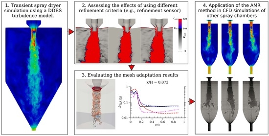
This paper proposes the application of AMR methods to reduce computational costs in transient simulations of spray dryers. To the authors’s knowledge, the application of AMR methods in spray dryer simulations is a novel approach. Consequently, there is uncertainty about whether using specific AMR configuration parameters that have demonstrated effectiveness in other applications will be suitable in this context. This study evaluates three refinement criteria and two AMR configuration parameters to model airflow in two distinct spray drying chambers operating with a co-current flow configuration. The criteria for evaluation are based on the relative errors associated with velocity gradient, pressure gradient, and vorticity, while the AMR configuration parameters are the refinement level and threshold. The first drying chamber is of pilot size, has an annular inlet with Re = 19,600, and has been studied by Gutiérrez Suárez [27] and by Benavides-Morán et al. [18]. The second drying chamber is of semi-industrial size, has an annular inlet with Re = 41,200, and was studied by Kieviet [3]. For both drying chambers, the cited studies provide experimental airflow data obtained by hotwire anemometry (HWA), serving as a base for validation. To account for the unsteady nature of the internal airflow, a transient modeling approach in a fully three-dimensional domain is used. Turbulence resolution capability is provided by a delayed-DES model, which is suitable for the simulation of spray dryers [26]. Special attention is paid to the full development of flow instabilities. The primary objective is to determine an AMR configuration that reduces the computational costs of transient CFD simulations of spray dryers while maintaining solution accuracy.
This paper is organized into five sections. Section 2 provides a description of the numerical methods employed in the study. In Section 3, the computational configuration is discussed, including details about the domain, base grid, and boundary conditions. Section 4 outlines the numerical experiments and the simulation methodology employed. The results and discussion are presented in Section 5, where the evaluation of each AMR criterion, threshold values, and refinement limits are discussed. Finally, Section 6 presents the conclusions derived from the study.

2. Numerical Methods and Turbulence Modeling

2.1. Governing Equations and Turbulence Modeling

The governing equations for this problem are the incompressible-flow unsteady Navier–Stokes equations for continuity (Equation (1)) and momentum (Equation (2)):
u i x i = 0
u i t + u i u j x j = 1 ρ p x i + ν + ν u i x j .
Due to the use of a hybrid LES/RANS turbulence model, these equations may adopt unsteady RANS and filtered (LES) formulations through the domain (see [26,28]). In URANS, an averaging operation is performed on pressure and velocity terms ϕ n = ϕ n , and the modeled viscosity ν is replaced by the turbulent viscosity ν T , which is calculated by the RANS turbulence model. In LES mode, spatial filtering is used, with ϕ n = ϕ n ¯ , and the modeled viscosity ν is replaced by the sub-grid scale (SGS) viscosity, with ν = ν SGS , calculated by the delayed-DES model.
The delayed-DES (DDES) model is classified as an interfacing LES/RANS turbulence formulation [29]. This model is characterized by an improved behavior in near-wall regions, avoiding an early switch from RANS to LES mode [30]. The early switching may happen in conditions of low-flow instabilities or thick boundary layers. This near-wall functionality under very coarse grids has been verified in a prior work by Gutiérrez Suárez et al. [26]. In the SST-DDES model, the transport equation for the turbulent kinetic energy (k) is defined as:
ρ k t + ρ u j k x j = ρ p D DDES k + μ + μ t σ k k x j x j .
Here, the term D DDES k represents a relation between RANS and LES turbulence length scales:
D DDES k = ρ k 3 / 2 / l DDES ,
with
l DDES = l RANS f d max ( 0 , l RANS l LES ) .
In this equation l RANS is the length scale defined for the SST k ω model as l RANS = k / C μ ω . l LES is defined in terms of a model constant C DES and the local maximum grid spacing Δ as l LES = C DES Δ . The empirical delay function f d protects the boundary layers from switching into LES mode. This function includes a correction ratio, which includes the molecular and turbulent viscosities, the strain-rate and vorticity vectors, and the distance to the nearest wall. Additional details of the DDES model, including the values of its constants, can be found in Gritskevich et al. [31].

2.2. Adaptive Mesh Refinement

The quantitative error analysis performed by Gutiérrez Suárez et al. [26] when numerically studying an annular swirling jet gives insight about key zones, where refinement would have a larger impact on improving the solution accuracy. These zones were found to be high-shear regions, where the high-velocity jet interacts with its lower-velocity surroundings and regions with high velocity and pressure fluctuations, such as those found beneath the bluff-body. In order to prioritize the refinement in these regions, three sensors are used for adaptation, of which two are based on gradient (velocity and pressure fields) and the third on vorticity.
A general refinement strategy based on Bathe and Zhang [22] is implemented in this work. This criterion determines whether or not an element should be refined/unrefined according to its local error. For any grid element, the local error c l is defined in terms of its mean edge length Δ l and the norm of a flow-solution variable in the element F e as:
c l = Δ l F e .
The flow-solution variable F e will be defined in this paper in terms of the velocity gradient U , the pressure gradient p , or the vorticity Ω . For the whole domain, an averaged error c avg can be determined from the local error c l of each of the grid elements as:
c avg = 1 N e e Δ l F e ;
here, N e represents the actual number of grid elements. Defining the error relation for any grid element as:
c rel = c l / c avg ,
the decision whether to refine a grid element or not is established in terms of a given refining criterion c crit . If c rel > c crit , the local element is refined. The selection of this refinement criterion is dependent on the case and physical phenomenon represented. Its value should be weighted according to the maximum level of refinement and the computational resources available.
Cell unrefinement occurs when c rel < c un , where c un represents an unrefinement criterion, assumed in this study as c un = 0.75 c crit . This selection is experience-based, enabling a balance between the number of refined elements and the desired refinement coverage. Increasing this value may amplify instabilities and lead to additional numerical fluctuations, whereas decreasing this value would keep cells refined where the relative error is not significant, resulting in inefficiency in the grid adaptation process. The selected value presented a good tradeoff between these discussed effects across all the studied cases.
Because the value of c rel changes for different flow velocities and annular jet configurations, in this paper, a better definition is given using the Reynolds number as:
C crit = c crit R e , C rel = c rel R e .

2.3. Numerical Schemes and Methods

The open-source CFD software OpenFOAM V1706 was used to solve the governing equations (Equations (1) and (2)). The viscous terms were resolved using DES-based turbulence models. The discretization methods for different terms are presented in Table 1. All temporal and spacial terms used are second-order accurate. The pressure–velocity coupling was achieved using the PIMPLE algorithm. The PIMPLE algorithm, described in Holzmann [32], is a combination of SIMPLE and PISO algorithms. This algorithm allows running transient problems under large Courant numbers. For pressure and velocity, the settings used for residual control include a solver tolerance of 1.0 × 10 05 , a relative tolerance of 0.001 , and a maximum number of iterations of 10 (per outer PIMPLE loop). Adaptive mesh refinement (AMR) is implemented through relative error criteria (see Equations (6)–(9)). These equations were incorporated into the OpenFOAM solver pimpleDyMFoam and compiled as a new solver for the purposes of the present study.

3. Computational Configuration

3.1. Flow Configuration and Domain

The modeling of the airflow (cold flow) is performed in two spray drying chambers, whose geometries and domains are presented in Figure 1. Both drying chambers are of co-current type and have an annular inlet. A significant portion of the annular duct is included in order to develop the flow before it is discharged into the chamber. The flow characteristics and annular jet geometries for both dryers are presented in Table 2. For the semi-industrial-size dryer, the flow velocity measured at the discharge [35] was used as a reference. With this value and assuming a developed turbulent velocity profile [36], the volumetric flow rate upstream Q = 0.377   m 3 s 1 was calculated. This value is approximately 10 times higher than that of the pilot-size chamber. Because Kieviet et al. [35] removed the upper section of the air disperser, where the swirl vanes are located, this case was modeled without swirl.
For the pilot-size dryer, the values reported in Benavides-Morán et al. [18] were used, with the exception of the swirl number at the jet discharge, which was obtained from the experimental measurements of Gutiérrez Suárez [27]. The swirl number S n at the discharge was calculated using the reported value of 238 RPM through the following equation:
S n = 0 R ρ U x U θ r 2 d r R 0 R ρ U x 2 r d r .
Table 2 presents the flow and geometry characteristics of the annular entrances for the pilot-size and semi-industrial-size spray drying chambers.
The same boundary condition (BC) types were used for both drying chambers. For the air inlet, a constant volumetric flow condition was used. As was done in Gutiérrez Suárez et al. [26], turbulent variables k and ω were defined through a fixed-value BC using very low initial values ( 1 × 10 6 ) . These values are expected to develop throughout the inlet duct, all the way to discharge. In the walls, the velocity was defined through a no-slip BC, which enforces a Dirichlet-type BC ( U x , θ , r = 0 ) . Turbulence variables k and ω were defined in this zone through standard wall functions.For the outlet, a zero-gradient boundary condition was applied to the velocity and turbulence variables, while the pressure was defined through a fixed-value BC, with p outlet = 0 .

3.2. Grids

The base grids for both drying chambers are presented in Figure 2. Both grids are structured and include a prerefined (to level 1) region covering the inlet duct. (The level of refinement refers to the number of refinement operations performed on the base grid element and subsequently to the new elements created after each refinement operation. Therefore, a level 2 refined cell is created from a base cell (level 0) that was refined 2 times. During this operation, 64 cells are created from the original cell.) The operation was carried out to improve the accuracy and stability of the solution in the near-field of the jet during the initialization of the cases. Upon activation of the AMR, the refinement of this region was directly controlled by the mesh adaptation algorithm.
For both grids, the elements are concentrated in the jet discharge and in the outlet duct. A positive growth factor from this point towards the radial boundaries and the outlet was implemented. The growth factor was adjusted to maintain values of y + between 100 and 300 on the chamber walls following activation of the AMR, assuming a flow recirculation velocity of 0.5 m/s. Due to the use of adaptive meshing, the base grids (level 0, without prerefinements) are very coarse: the mesh of the pilot-size chamber has 27,550 cells and the grid of the semi-industrial-size chamber has 39,540 cells. The distribution of elements in axial, tangential, and radial directions is presented in Table 3. For the pilot-size chamber dryer, the mesh is completely structured and is composed of hexahedral cells. For the semi-industrial-size chamber, the outlet pipe crosses the conical section of the chamber and makes the construction of the mesh more difficult. In a previous study, Anandharamakrishnan et al. [38] used a hexahedral mesh for the cylindrical section and a tetrahybrid mesh for the bottom conical section. In the present study, a structured mesh composed of hexahedral cells is used as the background mesh, and the outlet pipe is incorporated using split-hexahedral cells.
Due to AMR, the number of grid elements varies dynamically depending on the value of the non-dimensional refining criteria C crit (see Equation (9)) and on the maximum refinement level allowed ref max . The aim of grid adaptation is to produce a numerical solution equivalent in accuracy to that which could be obtained if the entire grid was refined but using fewer elements. For this reason, grid independence is not evaluated by consecutively increasing the overall element level but by testing different AMR configurations and their effect on the accuracy of the results.
For reference, a global refinement of the base grids (up to level 2) would result in a number of elements comparable to that reported in other studies (see Table 4). For the pilot-size chamber, the resulting number of elements is similar to that reported by Benavides-Morán et al. [18]. For the semi-industrial-size chamber, the number of elements is higher than that reported by most previous studies and is similar to that used by Saleh [39]. However, the effective grid sizes when using AMR are significantly smaller (see Table 5).

4. Numerical Experiments

4.1. Study Cases

Table 5 presents the main characteristics of the studied cases. The initial seven cases are specifically centered around the pilot-size drying chamber. Case C, serving as a base case, employs a fixed mesh (without AMR) consisting of 1.75 million elements, achieved by a global refinement of all elements of the base grid to level 2. This reference case enables the evaluation of results variations upon the activation of AMR.
Cases C1, C2, and C3 evaluate the effect of using different flow-solution variables as the basis for AMR. In these cases, the maximum refinement level is 2, and the refinement threshold is adjusted to obtain around 300,000 grid elements. Cases C2-1 and C2-2 evaluate the effects of the threshold values and maximum refinement level over the solution. Case C2-1 maintains the variable flow solution of case C2 ( p ) but uses a higher refinement threshold, significantly reducing the number of typical grid elements. Case C2-2 also uses the same variable flow-solution as C2 and C2-1, but the maximum level of refinement is set to level 3. In this case, the refinement threshold is significantly increased to reduce the number of refined elements and obtain a computational cost similar to cases C1, C2, and C3. For Case C2-3, a fixed prerefinement is performed on the entire base grid (to level 1) and a further level of refinement is allowed (up to level 2). For the semi-industrial-size chamber, three cases were studied using the same variable flow-solution ( U ). These cases were selected to determine the effect of the threshold value on the numerical results in a different drying chamber.
For all cases with AMR, the mesh adaptation was triggered every five time steps ( t AMR = 5 Δ t ), with a two-cell refinement buffer around refined cells. This choice was experience-based and aimed to balance computational efficiency while preventing information loss caused by a slow response of the adaptation method to rapidly changing flow features. The maximum Courant number was set to Co max = 0.85 , primarily reached at the jet discharge, where the refinement behavior tended to be uniform. In other regions within the drying chamber, the maximum Courant number was significantly lower than the inverse of the adaptation time ( Co max < 1 / t AMR ), ensuring adequate time for the AMR method to react to dynamic flow changes. The choice of Co max was based on findings from a previous study [26]. While the PIMPLE algorithm permits the use of higher Co max values, configuring it in this manner is not recommended due to the generation of artificial fluctuations at the jet discharge and an excessive dissipation downstream [26].

4.2. Simulation Times and Sampling of Data

The simulation times in this study are described in terms of a non-dimensional characteristic time t c defined as:
t c = t s t f = t s Q / V c .
Here, t s represents the time elapsed since the start of the simulation, t f is the time to fill the chamber, Q is the volumetric flow rate at the inlet, and V c is the volume of the chamber. For the pilot-size chamber, t f = 12.81 s, and for the semi-industrial-size chamber, t f = 23.85 s. The characteristic time t c represents the non-dimensional time required to fill the chamber once. All cases are initialized from t c = 0 to t c = 0.5 without AMR and using the basic grid presented in Figure 2. Then, from t c = 0.5 to t c = 2.0 , all the elements are refined to level 1. After t c = 2.0 , the AMR method is activated and the cases are run up to t c = 5.0 using the specific configurations described in Table 5.
Data collection by the probes is active during the entire simulation. However, only the data obtained after 3.5 t c are used for the analysis of the internal flow pattern. The criteria to determine these sampling times are presented in the results Section 5.1. The data collected by the probes are the instantaneous flow velocity and the turbulent kinetic energy calculated by the RANS component of the SST-DDES model. These data are sampled at 100 Hz using probes distributed in different axial and radial positions. Figure 3 presents the axial sampling positions and radial paths for both drying chambers. For the pilot-size chamber, the measured axial positions are x = ( 0.1 , 0.2 , 0.3 , 0.6 ) m. A total of 15 probes were set per axial position. Because the flow pattern in this drying chamber is asymmetric (as the annular duct is not concentric), the same measurement positions reported in previous studies [18,27] were used, varying the tangential position for each radial position. For the semi-industrial-size chamber, the axial positions are x = ( 0.3 , 0.6 , 1.0 , 2.0 ) m, with the same radial arrangement used by Kieviet et al. [35]. The mean-velocity profiles were obtained by averaging the data sampled by each probe. This sampling frequency was ensured by a dynamic adjustment of the simulation time step size Δ t .

5. Results

5.1. Computational Costs

The simulations were conducted on the JFF2 cluster at the CTTC (Heat and Mass Transfer Technological Center) of the Polytechnic University of Catalonia. This cluster comprises a total of 128 nodes, each equipped with 2 AMD Opteron Quad Core processors and 16 GB of RAM. These nodes are interconnected via an Infiniband DDR 4X network with a latency of 2.6 microseconds and a bandwidth of 20 Gbits/s. Cases C1 to C3 and S1 to S3 were executed using six processors, while cases C2-1 and C2-2 used four processors. For case C (base case), 16 processors were employed. This selection of cores per case was made to maintain an optimal range of cells per processor across all computational cases. Consequently, it helped reduce bottleneck effects associated with parallel computing, enabling a consistent comparison of computational costs. Further information on HPC scalability and bottleneck effects in OpenFOAM can be consulted in Culpo [43].
Figure 4 presents the computational costs in terms of effective processor hours ( P H ) per characteristic time t c . For similar grid sizes, costs are slightly higher in the pilot-size dryer than in the semi-industrial dryer. This is probably because its annular section is comparatively smaller and thinner, thus requiring a smaller time step. Compared to the base case (C), the reduction in computational cost when using AMR is between 3.2 and 11 times. Case C2-2 (up to three refinement levels) is an exception. This indicates that solving a larger fraction of the turbulence brings with it a substantial increase in computational cost, even if fewer grid elements are used.
Compared to the base case (C), the reduction in computational costs primarily results from a decrease in the number of grid elements, significantly lowering the cost of each time step. On the other hand, the cost is not affected by the time step size, which remains unchanged. This occurs because the regions with the largest influence on the time step size (where the Courant number is the highest) tend to remain refined throughout the simulation. There is a minor additional cost associated with running the AMR algorithm, which counts as running an additional time step in terms of cost.

5.2. Flow Development and Sampling Times

This section presents the results of the time-dependent flow development in the pilot- and semi-industrial-size drying chambers. These results support the criteria to sample the data presented in Section 4.2. The development times are represented by a characteristic time t c and are presented for cases C and S2 in Figure 5. The mean axial velocity U x and its rms fluctuations are used to evaluate the evolution of the flow development. These values are presented in intervals using a moving window average.
Figure 5a presents the mean U x results for the pilot-size drying chamber. At the centerline ( r / R = 0 ), a stabilization in the sampled velocity values is observed after t c = 2.5 . At the recirculation region ( r / R = 0.96 ), there is an increasing trend in the velocity magnitude, which means that the recirculation zone is becoming stronger. For the same drying chamber, rms fluctuations of the axial velocity U x are presented in Figure 5b. It is observed that after t c = 2 , the values of the rms fluctuations in the centerline and the recirculation region achieve a semi-stable behavior.
Figure 5c presents the mean U x results for the semi-industrial-size drying chamber. In this case, a clear trend is not observed in the time evolution of the results of the measurement points at r / R = 0 and r / R = 0.866 . A slight decrease in the axial velocity values is observed in the central jet around t c = 3 , which is related to an increase in velocity magnitude in the recirculation zone. However, after this point, the velocity shows an increasing trend with a wavelike pattern. Because of this, the measurement was extended from t c = 5 to t c = 8 . The results of this extended measurement (average velocity over the range) are shown as pointed horizontal lines in Figure 5c. It is observed that the recirculation flow becomes stronger and that the velocity in the central zone ( r / R = 0 ) takes an intermediate value. Figure 5d presents the sampled values of rms fluctuations. A clear increasing trend is observed at the center point ( r / R = 0 ) and recirculation zone ( r / R = 0.866 ). The increasing trend is more marked at the recirculation point, although the slope decreases slightly after t c = 1.2 .
These results show that the flow structure inside the drying chamber requires considerable time to fully develop. They also present evidence that the fluctuations are self-sustained by finding a correlation between the fluctuations in the recirculation zone and at the central point. Based on a qualitative analysis of the results, for both cases, after 3.5 t c , a decrease in the variation of axial velocities and rms fluctuations per segment is observed. Therefore, this time is selected to start the sampling of data. Given the results presented here, where the most significant variations in velocities and rms fluctuations occur before t c = 1 , the choice of measurement times is considered sufficient for the purpose of this study. For simulations of other spray dryers under different operating conditions, a trade-off between computational costs, grid refinement, and measurement time should be made.

5.3. Typical Refinement Regions

5.3.1. Pilot-Size Spray Chamber

Figure 6 presents the transient behavior of the airflow inside the pilot-size chamber obtained from the base case. The ability of the model to resolve turbulence is observed, in which detached eddies are captured just downstream of the discharge (see Figure 6a). These eddies grow in size downstream as the jet decays. Regarding the velocity along the radial direction at x / H = 0.367 (see Figure 6b), strong flow asymmetry is observed from the centerline. This asymmetry is a usual behavior in actual spray dryers, but in this particular case, it is most likely amplified by the defect in the concentricity of the annular entrance (see Figure 1c). This leads to a strong deflection of the jet, which sometimes can result in velocities close to 0 in the centerline.
Figure 7a–c presents the effect of the refinement criteria ( U , p , Ω ) on the relative error fields C rel . This visualization is important because it gives insight into the nature of each of the criteria and the regions that would be selected for refinement ( C rel > C crit ) in case of using adaptive meshing.
The first evaluation of these relative error fields is performed on a computational solution developed on a fixed grid (case C), which is presented in Figure 7a,b. In the near-field of the jet (Figure 7a), the differences are mainly observed in two regions: in the inlet diffuser, including the jet discharge, in the air disperser, and in the cells near the wall. The regions marked for refinement by the vorticity and velocity gradient criteria are quite similar. Both criteria refine cells along a large section of the inlet duct, but this refinement is only performed in near-wall cells. These criteria also exhibit high values of C rel in the high shear stress zone downstream of the discharge, where the high-velocity flow interacts with the surroundings. In some cases, near-wall cells on the upper walls of the chamber are marked for refinement. This behavior is undesirable because such cells do not interact with high-flow velocities. It occurs mainly because of the high aspect ratio of the elements in this zone (see Figure 2a). Since the mean element length Δ l in Equation (6) is calculated from the cubic root of its volume Δ l = V c 3 , in cells with a high aspect ratio, the magnitude of the local error is overpredicted. Regarding the pressure gradient criterion, high values of C rel are presented in the entire lower section of the air disperser, near the jet discharge. This behavior differs from that of the other two criteria. Additionally, it does not present high values of C rel in the upper wall due to the condition imposed p = 0 on the walls, which hinders the refinement of these cells.
Downstream of the jet discharge (Figure 7b), the C rel fields generated by the U and Ω criteria remain similar. In both cases, some elements near the lower walls are refined, which is desirable if high velocities are present in those areas. In detail, the U criterion presents a slightly higher coverage of the far zone of the jet. To reach the same coverage, the Ω criterion would require a C crit threshold significantly lower than 240.
Figure 7c presents the effective C rel fields obtained using AMR for cases C1, C2, C3, C2-1, and C2-2 taken at t c = 3.0 . In general, for cases C1 to C3, the behavior in the inlet duct zone and at the jet discharge is very similar to that obtained for the base case (Figure 7a). Downstream, however, the zone selected for refinement ( C rel > C crit ) exhibits a smaller extent, covering less than half the height of the chamber and terminating abruptly. This limitation arises because the base grid in this instance is too coarse to raise the local error above the refinement threshold. Regarding C2-1 and C2-2 cases, they presented a much lower coverage, especially for case C2-2, limiting itself to the discharge and the very-near region of the jet.
Figure 7d presents the effective refined regions (in terms of the cell level) for all the cases related to the pilot-size dryer. A two-cell refinement buffer is implemented around each refined cell to ensure smooth grid transitions. For cases C1 to C3, this approach effectively enhances the refinement area around the jet discharge, containing more cells than those initially selected for refinement ( C rel > 320 ). However, this strategy proves less effective for the other cases (C2-1 and C2-3), particularly for case C2-2, where a refined region is not retained at the jet discharge. Because the level of refinement in the discharge is crucial for modeling the development and decay downstream of the annular jet, this behavior is deemed unsatisfactory. Downstream of the discharge, the extent of the refined zone is similar to that selected for refinement ( C rel > C crit ).
Overall, case C2-3 presents a superior behavior to all the other AMR cases in this region by avoiding an abrupt transition between the refinement zones. This behavior aligns with the C rel fields observed for the base case (Figure 7a,b), further affirming the previously mentioned influence of the background grid on grid adaptation behavior. Near the output duct, the pressure gradient criterion generates a homogeneous refinement, which contrasts with the velocity gradient and vorticity criteria exhibiting similar operating characteristics to those observed in the inlet duct.

5.3.2. Semi-Industrial-Size Spray Chamber

Figure 8 presents the temporal evolution ( t c = 4.5 , 5.5 , 6.5 ) of velocity contours and refinement regions for case S2. Figure 8a shows the instantaneous contours of absolute velocity. In the high-velocity jet, the formation of detached eddies is observed just downstream of the annular blockage. The size of these eddies increases downstream as the jet widens and decays. Some recirculatory phenomena in the periphery of the jet are also observed. These flow phenomena may be related to the zones chosen for refinement, as shown in Figure 8b. These zones are presented as contours of the relative error C rel . As shown in Equations (8) and (9), the values of C rel and C crit determine the refining operations through the domain. As expected, the higher relative errors are present in high-shear zones, which are related to the jet, eddies, and the walls of the domain. Compared to the pilot-size dryer, in this case, the entire jet discharge region is not selected for refinement. This is mainly due to two factors: the low production of turbulence upstream (a turbulence intensity at the discharge of 2%), which is influenced by the absence of inlet swirl, and a slow reattachment of the jet. This results in low-velocity gradients in the central section and hence low levels of refinement. The delay in jet reattachment is further exacerbated by the open bluff-body cover (it is not completely clear in the article of Kieviet et al. [35] if the cover of the bluff-body was left open; it was assumed that it was from the interpretation of the drying chamber figures and the computational grid presented in that study), generating large pressure fluctuations that prevent the two sections of the annular jet from merging.
Downstream of the discharge, some regions marked for refinement follow the large-detached eddies resolved by the DDES model. These refinement regions travel with the eddy until it loses energy and is dissipated. Regions marked for refinement are also observed around the outlet duct, including the pipe walls and below the outlet duct, where the flow experiences a sudden change in direction. Recirculation regions are not selected for refinement due to the low energy of recirculating eddies. However, some near-wall elements are marked for refinement in regions where flow impingement occurs. This occurs especially in the section where the shape of the chamber changes from cylindrical to conical and in the areas opposite the outlet duct. A correct capture of the flow behavior in these regions appears to have a significant effect on flow stability, as mentioned by Keshani et al. [42], making their refinement desirable.

5.4. Turbulence Resolution at the Jet Discharge

Table 6 presents some parameters related to turbulence resolution measured at the jet discharge for the pilot-size dryer. These parameters are the rms fluctuations of the axial velocity (rms U x ), the resolved turbulent kinetic energy ( k LES ) , the modeled turbulent kinetic energy k RANS , the total turbulent kinetic energy k, and the resolved turbulent kinetic energy fraction Γ . The resolved fraction is calculated from the resolved turbulent kinetic energy k LES and the modeled turbulent kinetic energy k RANS as:
Γ = k LES k LES + k RANS .
According to Pope [21], for a well-resolved LES simulation, Γ > 0.8 . For the base case (C), it is observed that the resolved fraction of turbulence is very low compared to a LES study ( Γ = 0.191). This means that only a small number of very large turbulent structures are being resolved and that most of the turbulent kinetic energy corresponds to the modeled fraction ( k RANS ). The low fraction of resolved turbulence is a consequence of the coarseness of the grids and the very low inlet swirl values. Increasing this resolved fraction would imply radically increasing the number of elements in the inlet duct region, which results in very large computational costs.
The effect of using the different AMR criteria (C1, C2, C3) is presented next. For rms U x , k LES , and k RANS , a substantial increase is observed when using any of the criteria, especially for p (case C2), where the generated rms U x fluctuations are much higher than those predicted with the fixed grid, and results in a generalized increase in the resolved turbulent kinetic energy k LES . Since the resolution of the grid is much the same as that of the reference case (case C), it is evident that a problem of artificial fluctuations is occurring, most likely due to drastic changes in the level of refinement in this critical zone. This leads to interpolation errors, which, in turn, cause artificial fluctuations. The increase is more marked in case C2 ( p criterion), possibly because, upstream of the discharge, the grid level changes more abruptly than for the other cases, as shown in Figure 7. For cases C1 and C3, the increase in rms U x does not produce an increase in Γ because the increase in k RANS is proportionally higher, making the Γ value lower than that of the base case (C). In case C3 ( Ω criterion), the increase in resolved turbulent kinetic energy k LES is greater than the increase in modeled turbulent kinetic energy k RANS , resulting in a total turbulent kinetic energy value similar to that of the base case.
Regarding cases C2-1 and C2-2, using a pressure gradient refinement criterion, and different threshold and maximum refinement level values, the following results are obtained. For case C2-1, using a larger threshold and consequently a smaller number of elements than in case 2, the rms U x values are increased. This occurs due to the lower coverage of refined regions in the input diffuser, limiting themselves to the jet discharge. Therefore, near the jet discharge, sudden changes in the refinement level and the mode of operation (RANS or LES) occur constantly, generating strong artificial oscillations. On the other hand, since most of the diffuser is unrefined to an extremely coarse, level 0 grid, the production of modeled turbulent kinetic energy k RANS is reduced. This is due to the incorrect calculation of wall shear stresses and low shear stresses between cell faces. The resulting overprediction of rms U x and underprediction of k RANS artificially increase the resolved fraction Γ . For case C2-2, where a higher level of refinement (level 3 refinement) is allowed, something similar happens. The resolved fraction of turbulence reaches a value of Γ = 0.71 , which is close to the required value for LES. Compared to the base case, the resolved turbulent kinetic energy k LES increases 12 times, and the modeled turbulent kinetic energy k RANS decreases by half. This increase in the resolved fraction is related to the finer grid but also to the same artificial fluctuations presented in case C2-1. For case C2-3, running under a more refined background grid, the values of k RANS and k are similar to those obtained in the base case, while k DES and Γ are slightly overpredicted. This indicates that the effect of the artificial fluctuations is less marked than in the previous cases, affecting only the resolved portion of the turbulence.
The various turbulence-resolving behaviors presented in the discharge have effects downstream. Visualization of coherent structures in the flow is used to observe these effects. Figure 9 presents these coherent structures downstream of the discharge. The coherent structures are colored by the instantaneous pressure value and are generated as iso-surfaces of the so-called Q-criterion. For the base case (without AMR) presented in Figure 9a, some vortical structures can be visualized, which break into smaller structures at the end. Comparatively, for the U criterion presented in Figure 9b, no such larger structures are observed, although the amount of smaller structures is qualitatively similar. For the pressure gradient criterion (Figure 9c), much larger structures are observed than in the base case, which is related to the stronger fluctuations (due to artificial effects already explained) and to higher rms values. Compared to the U case, the p case seems to present a smaller amount of smaller structures, which would explain why the k LES values are not so different. Regarding the Ω criterion, qualitatively, the behavior is similar to that of the base case, but the structures seem to be larger. Hence, the increase in the resolved fraction of turbulence would be due to the increase in the size of these structures due to artificial effects. From these results, it is concluded that abrupt transitions in refinement levels at the discharge are not desirable due to the negative effect downstream.

5.5. Effects of the AMR Approach on the Mean Axial Velocity Profiles and Turbulence Resolution in the Pilot-Size Spray Chamber

5.5.1. Mean Axial Velocity Profiles

Figure 10 presents the effects of the different AMR criteria on the radial profiles of the axial velocity U x in the pilot-size chamber. For comparison purposes, the experimental HWA data reported by Gutiérrez Suárez [27] are included. Overall, no significant differences are observed between the results predicted by the reference case without AMR (case C) and the cases using AMR (C1, C2, C3). It is observed that at lower axial positions (starting at x / H = 0.22 ), case C1 ( U criterion) underpredicts the jet decay rate, while case 2 ( p criterion) predicts a higher decay rate than the reference case. This is an effect of the overprediction on the turbulent kinetic energy in the discharge. Compared to experimental measurements, the CFD results underpredict the jet decay and widening, which is evident from x / R = 0.147 . This behavior has been observed in computational studies of average velocities for this and other spray chambers and is explained in part by the mesh resolution requirements in the near-field of the annular jets.
Still, for the pilot-size spray chamber, these results are an improvement over those obtained in a previous study [18], as presented in Figure 11.

5.5.2. Turbulence Statistics

Figure 12 presents the radial profiles of the fraction of the resolved turbulent kinetic energy Γ for the base case (case C) and AMR cases (C1, C2, and C3) obtained in different axial positions downstream of the jet discharge. In general, it is observed that the base grid (case C) presents the best overall results in terms of the portion of turbulence resolved. This result is expected since it has all elements refined to level 2 in a fixed grid. For all cases, close to the discharge ( x / H = 0.073 and r / R = 0 to 0.15), the resolved fraction Γ varies between 0.8 and 0.9. This stands in contrast to the results presented in Table 6, where much lower values were obtained. For all cases, this value becomes larger at lower axial positions, being close to 1.0. This is explained by the transition to larger turbulent structures, which are better captured in lower axial positions by maintaining grid resolution. In this zone, case C2 (criterion p ) predicts a higher fraction of turbulence than the reference case. This is most likely due to the abrupt change in the level of refinement in the outflow duct, which generates some artificial oscillations. Outside the central jet ( r / R > 0.2 ), all criteria would be expected to have a lower resolved fraction than the base case (case C) since they do not explicitly refine the recirculation zone. However, the p criterion predicts at various times higher resolved fraction values than the base case, indicating that the artificial fluctuations generated in the discharge also affect the recirculation zone. For this zone, the vorticity criterion offers the best results.

5.6. Effects of the Refinement Threshold and Cell Level

5.6.1. Pilot-Size Spray Chamber

Axial Velocity Profiles

Figure 13 presents the effects of using a lower threshold (case C2-1) and different refinement settings (cases C2-2 and C2-3) on the mean axial velocity U x . For comparison purposes, data from cases C and C2 are included. Overall, cases C2-1 and C2-2 offer a similar behavior at all axial positions, predicting lower axial velocities than the base case (C). On the other hand, the C2-3 case predicts very similar results to those obtained by the base case. The apparent improvement in the results predicted by cases C2-1 and C2-2 is most likely due to incorrect turbulent kinetic energy production in the jet discharge (see Table 6), along with low refinement coverage in the jet (see Figure 7d), as discussed in the next section.

Turbulence Statistics

Figure 14 presents the radial profiles of the fraction of the resolved turbulent kinetic energy Γ for cases C, C2, C2-1, C2-2, and C2-3. In the high jet velocity zone, cases C2-1 and C2-2 present a similar behavior, predicting lower resolved fraction values than the reference cases (C and C2). This is especially noticeable in the high shear stress zone that marks the periphery of the jet with its surroundings ( x / H = 0.147 , 0.22 ; r / R 0.25 ), indicating a significative coarseness of the grid. On the other hand, in these regions, case 2-3 presents similar results to those of the base case. In the recirculation zone, which starts at r / R 0.25 in the upper lines and r / R 0.45 in the lower lines, different behaviors are presented. In this region, cases C2-2 and C2-3 tend to predict higher resolved fractions than that of the base case. This behavior is explained by Figure 15, showing that the increase of the resolved fraction in the recirculation region is related to a decrease in the turbulent kinetic energy k RANS values. On the other hand, case C2-1 underpredicts the resolved fraction in all regions and axial positions. It is concluded that the discrepancies obtained are due to insufficient mesh coverage and abrupt transitions in the mesh refinements in the initial region of the jet, which are more evident for cases C2-1 and C2-2 than for C2-3. Moreover, turbulence resolution quality indicators should be analyzed comprehensively. For example, for C2-1 and C2-2, the maximum discrepancy with case C results in the resolved fraction of the near-jet region ( x / H = 0.147 , r / R < 0.2 ) being less than 10%, while for the modeled kinetic energy ( k RANS ), it is more than 250% (Figure 15).

5.6.2. Semi-Industrial-Size Spray Chamber

Axial Velocity Profiles

Figure 16 presents the radial profiles of the mean axial velocity at five different axial positions. Overall, the CFD results follow well the trend of experimental data. Compared with the experimental data, in the central jet, in the near-field region ( x = 0.3 m ) , all cases predict well the characteristic shape of the annular jet, with higher velocities below the annular entrance and lower below the bulk-body. From x / H = 1.0 , all cases overpredict the experimentally measured mean velocity values. Although experimental measurements of mean velocity are unavailable at x / H = 1.4 and x / H = 2.0 , the CFD predicted values appear similar to the maximum measured values, thus are assumed to be higher than the mean velocity. The differences in the results among different AMR thresholds are very small. It is observed that the S2 and S3 cases behave almost identically, while the S1 case predicts slightly lower decay rates in the central region. This is most evident at x / H = 0.536 and r / R = 0 , where case S3 predicts a velocity 10% larger than cases S1 and S2. In the recirculation zone, the velocity predicted by case S3 tends to be lower than for cases S1 and S2. In summary, using a higher refinement threshold (case S3) reduces the decay rate of the main jet and generates lower velocities in the recirculation zone.
Figure 17 compares the results obtained from case S3 with the results obtained by other studies. Details of these studies can be consulted in Table 4. At x = 1.0 m, the velocity profile predicted by case S3 is very similar to the one reported by the transient simulation of Saleh [39], which used three times more grid elements. At x = 2.0 m, case S3 has a much better prediction of the radial velocity profiles than those reported by Anandharamakrishnan et al. [38] and by Huang et al. [40], which use a steady-state approach. In these studies, the asymmetry of the jet appears exaggerated, which might be related to a non-converged solution. A more extensive comparison with results from other studies was not performed since the vast majority of those do not use a three-dimensional transient approach. In addition, many papers do not report results at lower axial positions, limiting the discussion to upper lines ( x = 0.3 ; 0.6 ), where discrepancies are less significant.

Velocity Intervals: Comparison with Experimental Data

Figure 18 presents the radial profiles of axial velocity intervals at different axial positions. In general, using lower C crit threshold values increases the maximum axial velocity at most measurement positions. This is especially noticeable in the high-shear zone, where the jet interacts with its surroundings, and in the recirculation zone. In high-shear zones ( r / R 0.15 ) , the maximum velocity values predicted with case S3 are up to 80% higher than those of case S1. Nonetheless, around the jet and towards the walls, all cases follow well the pattern of the measured velocity intervals.

6. Conclusions

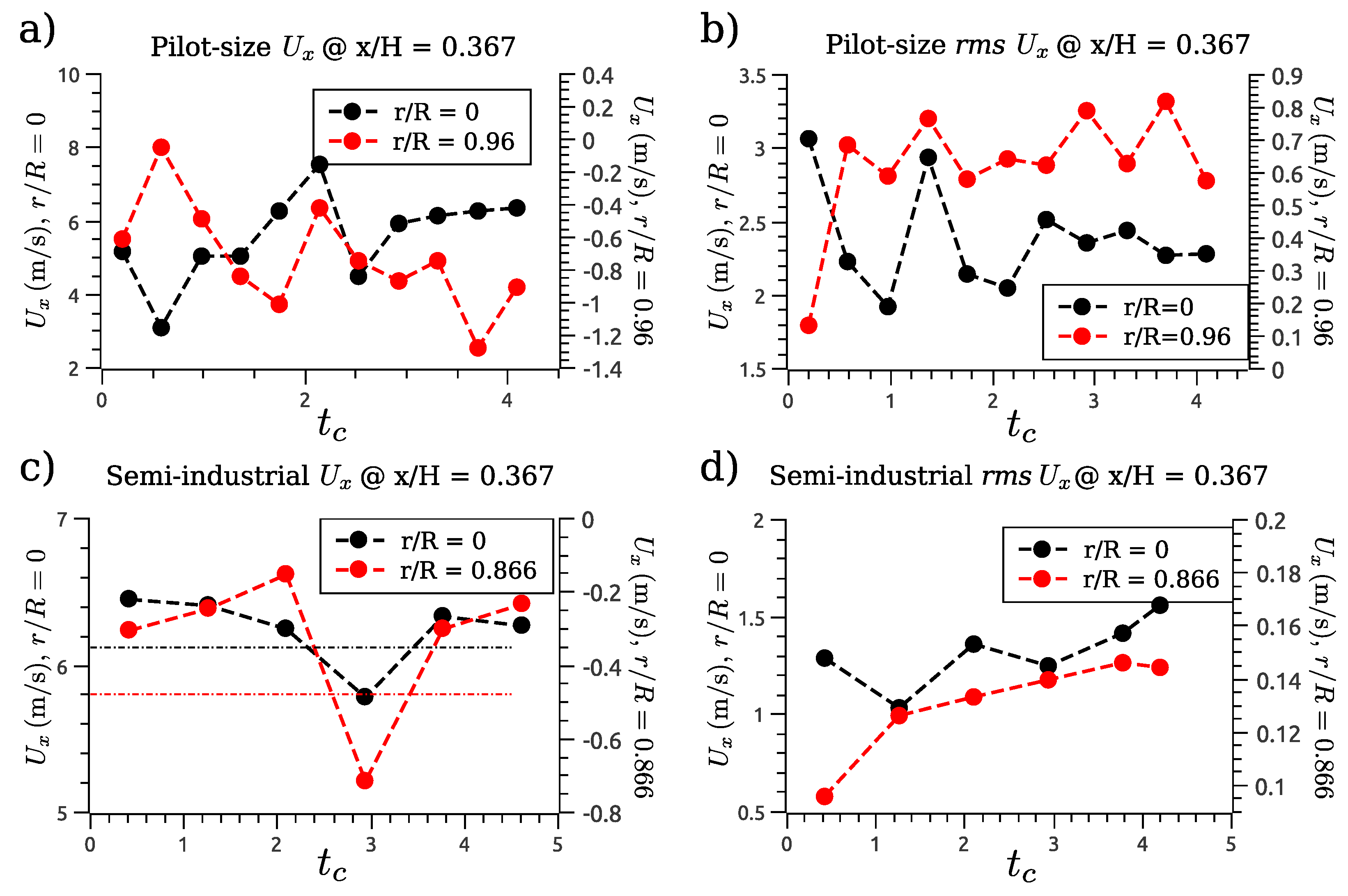
In this study, adaptive mesh refinement (AMR) is used in conjunction with a hybrid LES/RANS turbulence model to simulate the airflow in two different spray drying chambers. The use of AMR allowed a significant computational cost reduction. Compared to the base case (fixed grid with two refinement levels), the cases evaluated showed a 70% to 91% reduction in computational cost. This computational cost reduction becomes critical due to the long simulation times required to develop the internal flow ( t c > 2.5 ). The AMR approach presented in this study can be used in parametric studies of spray drying processes and other confined jet applications where computational costs become a major limiting factor. In this way, it is possible to run numerous simulation cases using a high-end workstation. However, cost reduction strategies must be accompanied by a careful application of the AMR methods to avoid an impact on the accuracy of the results.
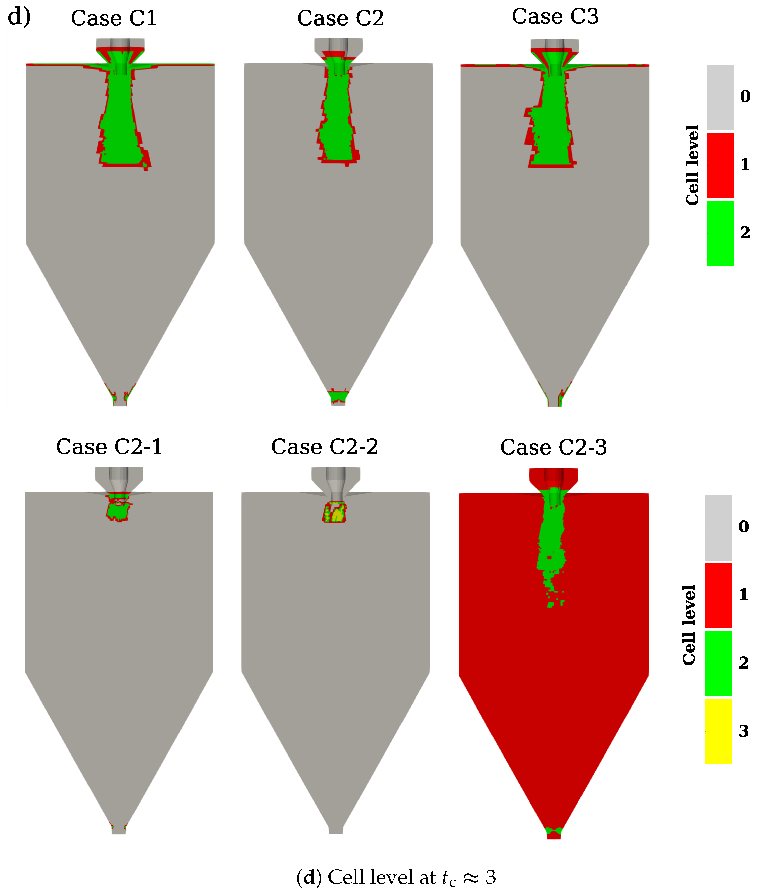
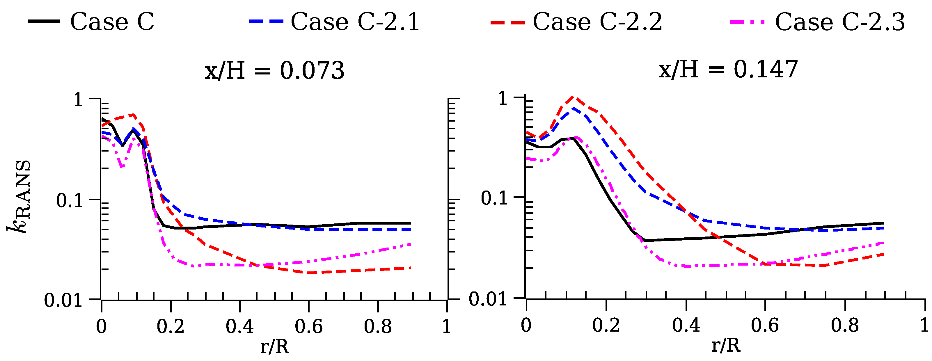
In general, the effect of different factors on mesh adaptation behavior must be assessed for all the criteria evaluated. In the absence of swirl at the discharge (as is the case in the semi-industrial-size dryer), the radial coverage of the refining zone is very different from that obtained in a low-swirl jet (pilot-size chamber). The size of the background grid (level 0) is also influential, since if it is excessively coarse, a sufficiently high relative error will not be generated to trigger the mesh adaptation. Finally, the refinement threshold must also be balanced against the maximum refinement level allowed. Based on the results of this study, it does not always seem appropriate to reduce refinement coverage by a higher level of refinement. It is estimated that the ideal refinement threshold should generate a grid containing between 25% and 40% of the elements of a fixed grid. The use of lower threshold values, such as that of case S3, which generates a grid with a proportion greater than 40%, does not seem to bring a noticeable improvement in the results.
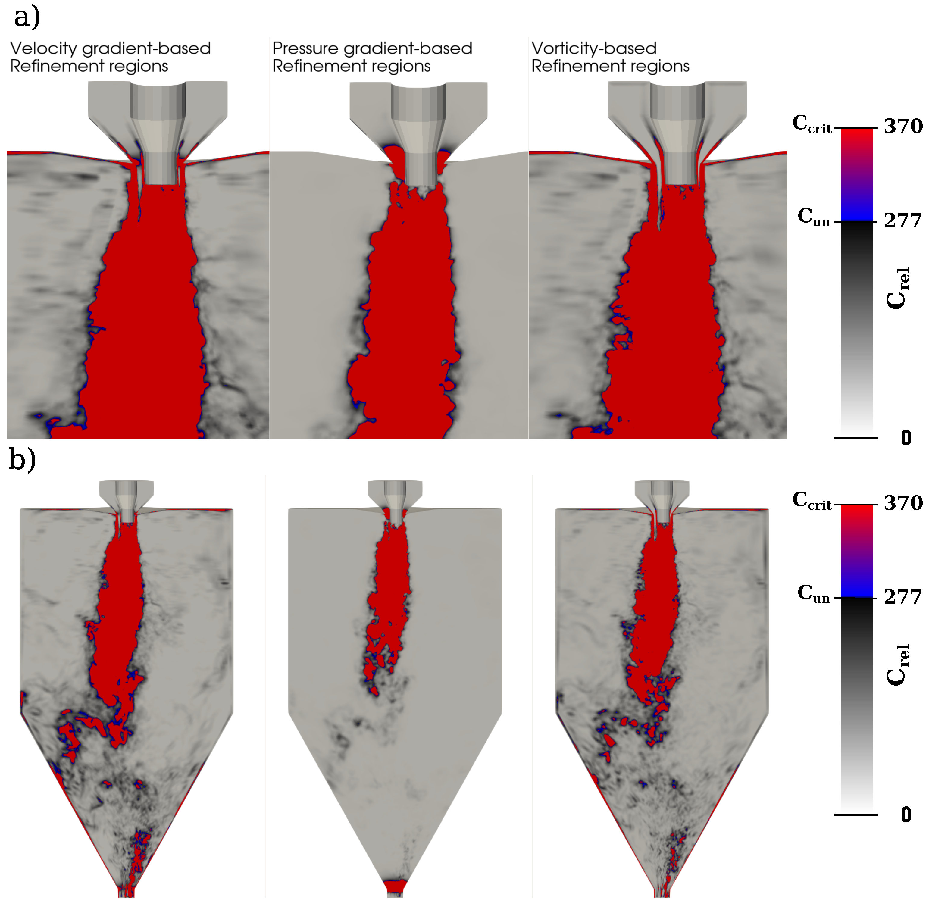
In detail, the differences in results when using various AMR criteria ( U , p , Ω ) are small but significant. At first glance, the pressure gradient-based criterion allows for a better modeling of the jet discharge by ensuring its complete refinement. However, the transition between different refinement levels is abrupt, generating artificial oscillations. Moreover, as it focuses solely on a narrow region, at the jet discharge, it inaccurately models the kinetic energy k RANS upstream. Both the U and Ω criteria generate a smoother transition between refinement levels in the inlet duct but are not consistent in refining to the highest level of the section with the highest axial velocity in the discharge. Due to these sporadic changes in the level of refinement, some artificial fluctuations are generated but of lesser intensity than in the case of the p criterion. To eliminate or reduce these fluctuations, there are several alternatives: The first one is to carry out a fixed prerefinement in the cells around the inlet diffuser. In this way, AMR-controlled unrefinement would not be allowed in such cells, and these artificial fluctuations would be eliminated. According to the results of Mozaffari et al. [24], it is recommended to extend the prerefining to the recirculation zone under the bluff-body to remove truncation errors due to the high flow instability; the second is to increase the number of buffer cells between cells with different refinement levels. In this way, the transition between cell levels would be smoothed, and the results of the p criterion would be enhanced; the third alternative is to combine the p criterion with one of the other two to generate a more homogeneous refinement in the discharge and in the near-region of the jet; the fourth is incorporating nonlinear terms in the relative error calculation, such as C rel = c rel R e 3 . This would smooth the transition between refinement levels and increase the coverage of transition cells.
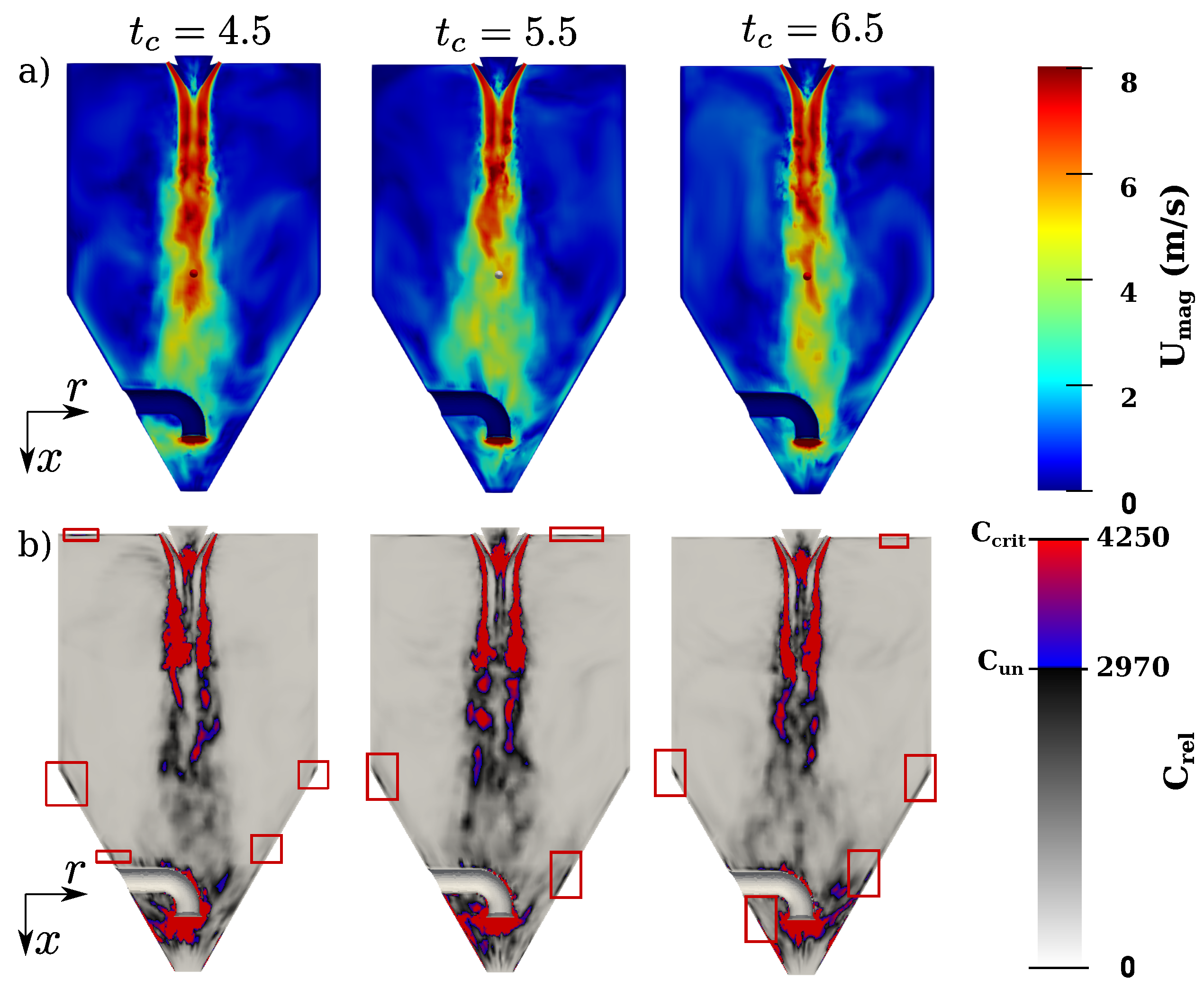
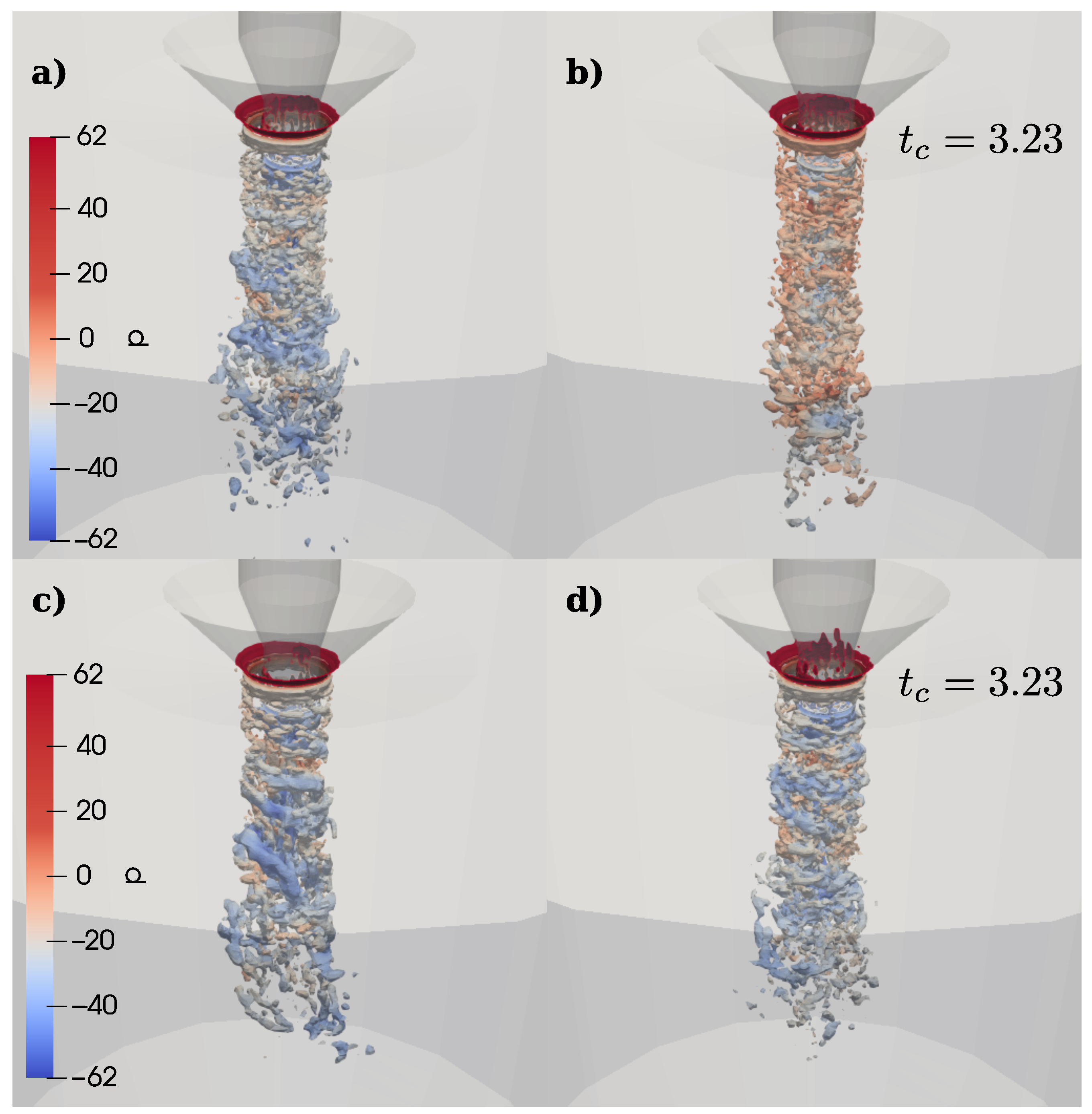
Downstream of the discharge, the cases with higher jet refinement coverage (C1–C3 and S1–S3) manage to capture by dynamic grid adaptation the transient motion of the jet. The operational differences between the AMR methods are mainly observed in their interaction with the walls. The criterion p does not perform refinements on the chamber walls (except for the inlet and outlet ducts). The U and Ω criteria do perform refinements on the walls. This can be an advantage in improving the accuracy of the results where there is impingement between the gas or particles with the chamber walls or internal ducts, as in the case of the semi-industrial-size dryer. Regarding the axial velocity profiles, all cases predict good results compared to experimental results and those obtained in previous studies. However, it is necessary to properly adjust the AMR method to reduce the generation of artificial oscillations in the jet discharge, which can potentially increase the turbulent kinetic energy dissipation rate and artificially increase the jet decay rate. To better assess this impact and improve the applicability of AMR methods along turbulence-resolving models in spray drying simulations, it is desirable that future work include experimental measurements of turbulence inside the chamber.

Author Contributions

Conceptualization, J.A.G.S. and C.H.G.U.; Methodology, J.A.G.S., A.G.M. and C.H.G.U.; Resources, A.G.M. and C.H.G.U.; Supervision, A.G.M. and C.H.G.U.; Software, J.A.G.S. and C.H.G.U.; Validation J.A.G.S.; Writing, J.A.G.S., A.G.M. and C.H.G.U.; Review and Editing. A.G.M. and C.H.G.U. All authors have read and agreed to the published version of the manuscript.

Funding

J.A. Gutiérrez acknowledges the PhD scholarship from COLCIENCIAS (PDBCNal, COLDOC-Convocatoria 647).

Acknowledgments

The authors wish to thank the CTTC—Centre Tecnològic de Transferència de Calor—Universitat Politècnica de Catalunya and Assensi Oliva for their support in economic, computational, and physical resources for the development of this study.

Conflicts of Interest

The authors declare no conflict of interest.

References

  1. Santos, D.; Maurício, A.C.; Sencadas, V.; Santos, J.D.; Fernandes, M.H.; Gomes, P.S. Spray drying: An overview. In Biomaterials-Physics and Chemistry-New Edition; IntechOpen: Londone, UK, 2018; pp. 9–35. [Google Scholar] [CrossRef]
  2. Sommerfeld, M. Modelling Requirements for CFD Calculations of Spray Dryers. Jornada em escoamentos multifásicos 2015. 2015. Available online: https://eventos.abcm.org.br/jem2015/KEYNOTES/K03_PRESENTATION.PDF (accessed on 26 September 2023).
  3. Kieviet, F. Modelling Quality in Spray Drying. Ph.D. Thesis, Eindhoven University of Technology, Eindhoven, The Netherlands, 1997. [Google Scholar] [CrossRef]
  4. Zbicinski, I. Modeling and scaling up of industrial spray dryers: A review. J. Chem. Eng. Jpn. 2017, 50, 757–767. [Google Scholar] [CrossRef]
  5. Kieviet, F.; Kerkhof, P. Air flow, temperature and humidity patterns in a co-current spray dryer: Modelling and measurements. Dry. Technol. 1997, 15, 1763–1773. [Google Scholar] [CrossRef]
  6. Woo, M.W.; Huang, L.X.; Mujumdar, A.S.; Daud, W.R.W. CFD Simulation of Spray Dryers; Number 1; National University of Singapore: Singapore, 2010; Chapter 1; pp. 1–36. Available online: https://www.yumpu.com/en/document/view/32880341/spray-drying-technologypdf-national-university-of-singapore (accessed on 26 September 2023).
  7. Southwell, D.; Langrish, T. Observations of flow patterns in a spray dryer. Dry. Technol. 2000, 18, 661–685. [Google Scholar] [CrossRef]
  8. Southwell, D.; Langrish, T. The effect of swirl on flow stability in spray dryers. Chem. Eng. Res. Des. 2001, 79, 222–234. [Google Scholar] [CrossRef]
  9. Fletcher, D.; Guo, B.; Harvie, D.; Langrish, T.; Nijdam, J.; Williams, J. What is important in the simulation of spray dryer performance and how do current CFD models perform? Appl. Math. Model. 2006, 30, 1281–1292. [Google Scholar] [CrossRef]
  10. Lebarbier, C.; Kockel, T.; Fletcher, D.; Langrish, T. Experimental measurement and numerical simulation of the effect of swirl on flow stability in spray dryers. Chem. Eng. Res. Des. 2001, 79, 260–268. [Google Scholar] [CrossRef]
  11. Langrish, T.; Williams, J.; Fletcher, D. Simulation of the effects of inlet swirl on gas flow patterns in a pilot-scale spray dryer. Chem. Eng. Res. Des. 2004, 82, 821–833. [Google Scholar] [CrossRef]
  12. Jin, Y.; Chen, X.D. A three-dimensional numerical study of the gas/particle interactions in an industrial-scale spray dryer for milk powder production. Dry. Technol. 2009, 27, 1018–1027. [Google Scholar] [CrossRef]
  13. Jongsma, F.; Innings, F.; Olsson, M.; Carlsson, F. Large eddy simulation of unsteady turbulent flow in a semi-industrial size spray dryer. Dairy Sci. Technol. 2013, 93, 373–386. [Google Scholar] [CrossRef]
  14. Fletcher, D.; Langrish, T. Scale-adaptive simulation (SAS) modelling of a pilot-scale spray dryer. Chem. Eng. Res. Des. 2009, 87, 1371–1378. [Google Scholar] [CrossRef]
  15. Afshar, S.; Jubaer, H.; Chen, B.; Xiao, J.; Chen, X.; Woo, M. Computational fluid dynamics simulation of spray dryers: Transient or steady state simulation? In IDS 2018 21st International Drying Symposium Proceedings; Editorial Universitat Politècnica de València: Valencia, Spain, 2018; pp. 395–402. [Google Scholar] [CrossRef]
  16. Lampa, A.; Fritsching, U. Large Eddy Simulation of the spray formation in confinements. Int. J. Heat Fluid Flow 2013, 43, 26–34. [Google Scholar] [CrossRef]
  17. Gimbun, J.; Muhammad, N.I.S.; Law, W.P. Unsteady RANS and detached eddy simulation of the multiphase flow in a co-current spray drying. Chin. J. Chem. Eng. 2015, 23, 1421–1428. [Google Scholar] [CrossRef]
  18. Benavides-Morán, A.; Cubillos, A.; Gómez, A. Spray drying experiments and CFD simulation of guava juice formulation. Dry. Technol. 2021, 39, 450–465. [Google Scholar] [CrossRef]
  19. Saleh, S.; Nahi Saleh, S. Transient simulation of air flow in a co-current spray dryer. In Proceedings of the European Drying Conference–EuroDrying, Palma, Spain, 26–28 October 2011; pp. 26–28. Available online: https://www.researchgate.net/publication/270506995_TRANSIENT_SIMULATION_OF_AIR_FLOW_IN_A_CO-CURRENT_SPRAY_DRYER (accessed on 26 September 2023).
  20. Antepara, O.; Lehmkuhl, O.; Borrell, R.; Chiva, J.; Oliva, A. Parallel adaptive mesh refinement for large-eddy simulations of turbulent flows. Comput. Fluids 2015, 110, 48–61. [Google Scholar] [CrossRef]
  21. Pope, S.B. Ten questions concerning the large-eddy simulation of turbulent flows. New J. Phys. 2004, 6, 35. [Google Scholar] [CrossRef]
  22. Bathe, K.J.; Zhang, H. A mesh adaptivity procedure for CFD and fluid-structure interactions. Comput. Struct. 2009, 87, 604–617. [Google Scholar] [CrossRef]
  23. Muralidharan, B.; Menon, S. Large eddy simulation of turbulent reacting jet in cross flow with adaptive mesh refinement. In Proceedings of the 52nd Aerospace Sciences Meeting, National Harbor, MD, USA, 13–17 January 2014; p. 0825. [Google Scholar] [CrossRef]
  24. Mozaffari, S.; Visonneau, M.; Wackers, J. Average-based Adaptive Grid Refinement in Hybrid LES. In Direct and Large Eddy Simulation XII; García-Villalba, M., Kuerten, H., Salvetti, M.V., Eds.; Springer Nature: Cham, Switzerland, 2020; Volume 27, pp. 449–455. [Google Scholar] [CrossRef]
  25. Wackers, J.; Visonneau, M.; Ali, Z. Automatic grid adaptation for unstructured finite volumes. Int. J. Eng. Syst. Model. Simul. 2010, 2, 2–11. [Google Scholar] [CrossRef]
  26. Gutiérrez Suárez, J.A.; Galeano-Urueña, C.H.; Gómez-Mejía, A. Low-Cost Eddy-Resolving Simulation in the Near-Field of an Annular Swirling Jet for Spray Drying Applications. ChemEngineering 2021, 5, 80. [Google Scholar] [CrossRef]
  27. Gutiérrez Suárez, J.A. Modelación CFD y validación experimental del proceso de evaporación de agua en un secador por aspersión. Master’s Thesis, Universidad Nacional de Colombia-Sede Bogotá, Bogota, Colombia, 2015. Available online: https://repositorio.unal.edu.co/handle/unal/56048 (accessed on 26 September 2023).
  28. Davidson, L. Fluid Mechanics, Turbulent Flow and Turbulence Modeling. Lecture Notes; Chalmers University of Technology. 2015. Available online: https://www.tfd.chalmers.se/~lada/postscript_files/solids-and-fluids_turbulent-flow_turbulence-modelling.pdf (accessed on 26 September 2023).
  29. Fröhlich, J.; von Terzi, D. Hybrid LES/RANS methods for the simulation of turbulent flows. Prog. Aerosp. Sci. 2008, 44, 349–377. [Google Scholar] [CrossRef]
  30. Travin, A.K.; Shur, M.L.; Spalart, P.R.; Strelets, M.K. Improvement of delayed detached-eddy simulation for LES with wall modelling. In Proceedings (CDROM) of the European Conference on Computational Fluid Dynamics ECCOMAS CFD, Egmond aan Zee, The Netherlands, 5–8 September 2006; Available online: https://www.cobaltcfd.com/pdfs/ECCOMAS_2006_improvement_DDESl.pdf (accessed on 26 September 2023).
  31. Gritskevich, M.S.; Garbaruk, A.V.; Schütze, J.; Menter, F.R. Development of DDES and IDDES formulations for the k-ω shear stress transport model. Flow Turbul. Combust. 2012, 88, 431–449. [Google Scholar] [CrossRef]
  32. Holzmann, T. Mathematics, Numerics, Derivations and OpenFOAM®, 4th ed.; Holzmann CFD: Loeben, Germany, 2017; Available online: https://www.academia.edu/download/56994390/MathematicsNumericsDerivationsAndOpenFOAM.pdf (accessed on 26 September 2023).
  33. Moukalled, F.; Mangani, L.; Darwish, M. Temporal Discretization: The Transient Term. In The Finite Volume Method in Computational Fluid Dynamics; Springer: Cham, Switzerland, 2016; pp. 489–533. [Google Scholar] [CrossRef]
  34. Travin, A.; Shur, M.; Strelets, M.; Spalart, P. Physical and numerical upgrades in the detached-eddy simulation of complex turbulent flows. In Advances in LES of Complex Flows; Springer: Dordrecht, The Netherlands, 2002; pp. 239–254. [Google Scholar] [CrossRef]
  35. Kieviet, F.; Van Raaij, J.; De Moor, P.; Kerkhof, P. Measurement and modelling of the air flow pattern in a pilot-plant spray dryer. Chem. Eng. Res. Des. 1997, 75, 321–328. [Google Scholar] [CrossRef]
  36. Okiishi, T.H. Fluid Velocity Profile Development for Turbulent Flow in Smooth Annuli; Digital Repository; Iowa State University: Ames, IA, USA, 1965. [Google Scholar] [CrossRef]
  37. Cubillos Varela, A. Modelación del proceso de deshidratación por espray de jugo de guayaba. Ph.D. Thesis, Universidad Nacional de Colombia, Bogotá, Colombia, 2017. Available online: https://repositorio.unal.edu.co/handle/unal/62971 (accessed on 26 September 2023).
  38. Anandharamakrishnan, C.; Gimbun, J.; Stapley, A.G.F.; Rielly, C.D. A study of particle histories during spray drying using computational fluid dynamic simulations. Dry. Technol. 2010, 28, 566–576. [Google Scholar] [CrossRef]
  39. Saleh, S.N. CFD simulations of a co-current spray dryer. World Acad. Sci. Eng. Technol. 2010, 62, 772–777. [Google Scholar] [CrossRef]
  40. Huang, L.; Kumar, K.; Mujumdar, A. A comparative study of a spray dryer with rotary disc atomizer and pressure nozzle using computational fluid dynamic simulations. Chem. Eng. Process. Process Intensif. 2006, 45, 461–470. [Google Scholar] [CrossRef]
  41. Noor, M.; Jolius, G. Detached eddy simulation (DES) of co-current spray dryer. Int. J. Technol. Manag. 2013, 2, 17–22. Available online: https://core.ac.uk/download/pdf/159178374.pdf (accessed on 26 September 2023).
  42. Keshani, S.; Montazeri, M.H.; Daud, W.R.W.; Nourouzi, M.M. CFD modeling of air flow on wall deposition in different spray dryer geometries. Dry. Technol. 2015, 33, 784–795. [Google Scholar] [CrossRef]
  43. Culpo, M. Current Bottlenecks in the Scalability of OpenFOAM on Massively Parallel Clusters. PRACE White Paper 2011. Available online: https://citeseerx.ist.psu.edu/document?repid=rep1&type=pdf&doi=308b983be3866f527931149b5686335fd8cb99b5 (accessed on 26 September 2023).
Figure 1. Geometry and domain of the two spray drying chambers modeled in this study. (a) Pilot-size co-current drying chamber studied by Benavides-Morán et al. [18], Cubillos Varela [37], Gutiérrez Suárez [27]. (b) Detail of the air disperser region featuring an annular inlet. (c) Defect in the concentricity of the annular entrance reported by Gutiérrez Suárez [27]. (d) Semi-industrial-size drying chamber studied by Kieviet et al. [35]. (e) Detail of the air disperser region. For both drying chambers, the position of the HWA probe during inlet air flow measurement is denoted by a red asterisk.
Chemengineering 07 00100 g001
Figure 2. Grid configuration for initial simulation setup (before AMR activation) in both drying chambers: (a,c), grid details in the near-field region of the jet, including the prerefinement, for the pilot-size and semi-industrial-size chambers; (b,d), cross-sectional view of the grid for the pilot-size and semi-industrial-size chambers. With the exception of the elements forming the outlet duct of the semi-industrial dryer, both grids are structured and concentrate the grid elements around the jet discharge and outlet duct regions.
Chemengineering 07 00100 g002
Figure 3. Axial positions and radial paths sampled in the CFD simulations. (a,b), sampled axial positions in the pilot-size and semi-industrial size spray chambers; (c,d), top view of the pilot-size and semi-industrial-size drying chambers showing the sampled path and some radial positions for reference. The sampled path replicates the movement of the hot-wire probe during the experimental measurements reported by Gutiérrez Suárez [27] and by Kieviet and Kerkhof [5].
Chemengineering 07 00100 g003
Figure 4. Computational costs in terms of the total processor hours per characteristic time ( P H / t c ) for all studied cases.
Chemengineering 07 00100 g004
Figure 5. Temporal evolution of mean and rms values of the axial velocity U x in the central jet and flow recirculation regions. For all cases, the x-axis represents the characteristic time t c . (a,b): mean and rms U x for the pilot-size drying chamber; (c,d) mean and rms U x for the semi-industrial-size drying chamber. The pointed horizontal lines in (c) represent the mean U x values when the simulation is run from t c = 5 to 8.
Chemengineering 07 00100 g005
Figure 6. Unsteady flow inside the pilot-size spray chamber at different characteristic times ( t c = 2.55; 2.95; 3.45) for the base case: (a) 2D cross-section of the contours of velocity magnitude; (b) axial velocity U x measured at x / H = 0.367 .
Chemengineering 07 00100 g006
Figure 7. Effect of the AMR criterion on the C rel fields and cell level for the pilot-size drying chamber taken at t c = 3 : (a,b) cross-section of the C rel fields for case C taken at t c = 3 ; (c) C rel for cases C1, C2, C3, C2-1, and C2-2; (d) fields of cell level for cases C1, C2, C3, C2-1, C2-2, and C2-3.
Chemengineering 07 00100 g007aChemengineering 07 00100 g007bChemengineering 07 00100 g007c
Figure 8. Unsteady flow inside the semi-industrial-size spray chamber and grid adaptation at different characteristic times ( t c = 4.5 ; 5.5 ; 6.5 ) for case S2: (a) 2D cross-section showing contours of absolute velocity; (b) 2D cross-section of the relative error C rel indicating zones subject to refining ( C rel > C crit ) and unrefining ( C un < C rel < C crit ).
Chemengineering 07 00100 g008
Figure 9. Coherent structures (contours with Q > 200,000 ) taken at t c = 3.23 for different study cases: (a) base case (case C); (b) case C1 ( U criterion); (c) case C2 ( p criterion); (d) case C3 ( Ω criterion).
Chemengineering 07 00100 g009
Figure 10. Radial profiles of the effects of the AMR criterion ( U , p , Ω ) on the mean axial velocity U x at different axial positions ( x / H = 0.073 , 0.147 , 0.22 , 0.367 ) of the pilot-size spray chamber. Black line: reference case (case C) using a fixed grid; blue, red, and green lines represent simulation data using different AMR criteria; black squares: experimental hot-wire anemometry data from Gutiérrez Suárez [27].
Chemengineering 07 00100 g010
Figure 11. Radial profiles of the mean axial velocity U x at two axial positions ( x / H = 0.22 , 0.294 ) for the pilot-size spray chamber. Blue line: reference case (case C) using a fixed grid; red line: CFD data reported in Benavides-Morán et al. [18] using a SAS (scale adaptive simulation) turbulence method; black squares: experimental hot-wire anemometry data from Gutiérrez Suárez [27].
Chemengineering 07 00100 g011
Figure 12. Comparison of the radial profiles of resolved turbulence fraction Γ obtained from the base case (C), and adaptive meshing criteria (C1, C2, and C3) at different axial positions.
Chemengineering 07 00100 g012
Figure 13. Radial profiles of the effect of the AMR threshold and maximum refinement level on the mean axial velocity U x at different axial positions ( x / H = 0.073 , 0.147 , 0.22 , 0.367 ) of the pilot-size spray chamber. Black line: reference case (case C) using a fixed grid; red line: higher threshold value (case 2-1); blue line: higher maximum refinement level (case 2-2); black squares: experimental hot-wire anemometry data from Gutiérrez Suárez [27].
Chemengineering 07 00100 g013
Figure 14. Radial profiles of the effect of the AMR threshold and maximum refinement level on the resolved fraction Γ at different axial positions ( x / H = 0.073 , 0.147 , 0.22 , 0.367 ) of the pilot-size spray chamber. Black line: reference case (case C) using a fixed grid; red line: higher threshold value (case 2-1); blue line: higher maximum refinement level (case 2-2).
Chemengineering 07 00100 g014
Figure 15. Radial profiles of the modeled turbulent kinetic energy ( k RANS ) for cases C, C2-1, and C2-2 at two different axial positions ( x / H = 0.073 , 0.147 ) of the pilot-size spray chamber. Black line: reference case (case C) using a fixed grid; blue dotted line: higher threshold value (case 2-1); green line: higher maximum refinement level (case 2-2).
Chemengineering 07 00100 g015
Figure 16. Radial profiles of mean axial velocity of the air ( U x ) at different axial positions x = ( 0.3 , 0.6 , 1.0 , 2.0 ) m. Red, blue, and green symbols represent cases S1, S2, and S3; black squares: hot-wire anemometry data from Ref. [5]; error bars: interval of axial velocities estimated from measurements by the same author.
Chemengineering 07 00100 g016
Figure 17. Radial profiles of mean axial velocity of the air ( U x ) at different axial positions x = ( 1.0 , 2.0 ) m. The results from case S2 are compared with the CFD results from [19,38,40].
Chemengineering 07 00100 g017
Figure 18. Radial profiles of maximum and minimum axial velocities ( U x ) at different axial positions x = ( 0.3 , 0.6 , 1.0 , 2.0 ) m. Red, blue, and green symbols represent cases S1, S2, and S3; error bars: interval of axial velocities measured by [5].
Chemengineering 07 00100 g018
Table 1. Numerical schemes and coupling methods used in the present study.
SchemesDescription
Temporal termsSOUE (Adams Moulton), second-order implicit, described in Moukalled et al. [33].
Gradient— ϕ CDS (central differencing scheme).
Gradient— u Limited-CDS.
Advective terms—div ϕ Hybrid scheme, described in Gutiérrez Suárez et al. [26], Travin et al. [34].
RANS modeLUD (linear upwind differencing).
LES modeCDS.
Pressure–velocity couplingPIMPLE algorithm, described in Holzmann [32].
Table 2. Flow and geometry characteristics of the annular entrances for the pilot-size and semi-industrial-size spray drying chambers.
DescriptionPilot-Size Spray Drying ChamberSemi-Industrial Spray Drying Chamber
Volumetric flow 0.0342   m 3 s 1 0.377   m 3 s 1
RPMs at the discharge2380
Swirl number0.0520
R o 0.0355 m0.244 m
R i 0.0260 m0.2024 m
D h = 4 A w e t / 2 π D a v g 0.0190 m0.084 m
Re19,60041,200
Reference air density 1.1 kg m 3 1.23 kg m 3
Kinematic air viscosity 1.42 × 10 5 m 2 s 1 1.48 × 10 5 m 2 s 1
Table 3. Total and direction-wise number of elements for the level 0 base grids of the pilot-size and semi-industrial-size drying chambers (without prerefinement). The elements of the air disperser are not included in the directional count.
Spray Drying ChamberElementsx θ r
Pilot-size chamber27,505881916
Semi-industrial-size chamber39,540521928
Table 4. Grid sizes, turbulence model, and time treatment in previous CFD studies of the pilot-size and semi-industrial-size drying chambers. For comparison purposes, the values used in the present study include a globally refined level 2 base grid. See Table 5 for the effective grid sizes when using AMR.
Drying ChamberAuthorYearGrid SizeTurbulenceTime
Pilot sizeGutiérrez Suárez [27]201512,672 (2D-axi-symmetric) k ϵ steady
Benavides-Morán et al. [18]20202,200,000SST k ω and SAStransient
Present study (level 2 refined base grid)20231,750,000SST-DDEStransient
Semi-industrial sizeHuang et al. [40]2006not reported k ϵ steady
Anandharamakrishnan et al. [38]2010294,237 k ϵ steady
Saleh [39]2010840,000 k ϵ transient
Noor and Jolius [41]2011503,000SA-DEStransient
Saleh and Nahi Saleh [19]2011516,000RNG k ϵ transient
Gimbun et al. [17]2015420,000SA-DEStransient
Keshani et al. [42]20151,223,675 (Case A)RNG k ϵ transient
Present study (level 2 refined base grid)2023736,000SST-DDEStransient
Table 5. Study cases for the pilot-size and semi-industrial-size spray chambers.
Pilot-size drying chamber
CaseNumber of cellsAMR flow variable C crit Max. refinement levelTurbulence
C (base)1,750,000fixed grid-Level 2 globally refined base gridDDES
C1300,000 U 370 (ref)2DDES
C2300,000 p 3702DDES
C2-178,000 p 37002DDES
C2-2180,000 p 37003DDES
C2-3380,000 p 3702 using a level 1 globally refined base gridDDES
C3300,000 Ω 370 (ref)2DDES
Semi-industrial-size drying chamber
S1170,000 U 12,3602DDES
S2220,000 U 41202DDES
S3378,000 U 12362DDES
Table 6. Turbulence-related parameters measured at the discharge of the jet for all study cases of the pilot-size spray drying chamber.
Referencerms  U x k LES k RANS k Γ
C0.00520.01860.07890.0970.191
C10.00730.02710.24430.2710.100
C20.01410.02330.32890.3520.066
C30.01100.02650.09500.1220.218
C2-10.01460.01560.02470.0400.387
C2-20.04160.12390.04920.1730.716
C2-30.07110.02250.075080.0950.237
Disclaimer/Publisher’s Note: The statements, opinions and data contained in all publications are solely those of the individual author(s) and contributor(s) and not of MDPI and/or the editor(s). MDPI and/or the editor(s) disclaim responsibility for any injury to people or property resulting from any ideas, methods, instructions or products referred to in the content.

