Pseudo-Spatially-Distributed Modeling of Water Balance Components in the Free State of Saxony

Abstract

Highly-resolved data on water balance components (such as runoff or storage) are crucial to improve water management, for example, in drought or flood situations. As regional observations of these components cannot be acquired adequately, a feasible solution is to apply water balance models. We developed an innovative approach using the physically-based lumped-parameter water balance model BROOK90 (R version) integrated into a sensor network platform to derive daily water budget components for catchments in the Free State of Saxony. The model is not calibrated, but rather uses available information on soil, land use, and precipitation only. We applied the hydro response units (HRUs) approach for 6175 small and medium-sized catchments. For the evaluation, model output was cross-evaluated in ten selected head catchments in a low mountain range in Saxony. The mean values of Kling–Gupta efficiency (KGE) for the period 2005–2019 to these catchments are 0.63 and 0.75, for daily and monthly discharge simulations, respectively. The simulated evapotranspiration and soil wetness are in good agreement with the SMAP_L4_GPH product in April 2015–2018. The study can be enhanced by using different data platforms as well as available information on study sites.

1. Introduction

Spatiotemporal information of water balance components is important for many aspects of water management, hydrological modeling, and forest management [1,2,3]. It often serves as the initial information used by hydrological models to describe discharge generation processes [4,5] and, thus, can be applied in the impact assessment of flood events. However, information on precipitation, evapotranspiration (ET), and soil moisture (SM) on a regional scale are increasingly important for assessing droughts as well [6,7,8]. This is especially the case in Europe, which has suffered in various economic and social sectors in recent years due to ongoing droughts, even though it is considered a water-rich continent [9,10]. With the increasing effects of climate change, the need for regional hydrological information becomes more relevant because of the high intensity of the increase of all kinds of water-related extreme events [11,12].

The ability to describe the water balance on a regional level thoroughly is linked to the information availability of its components. While precipitation, main driver of the water balance, and discharge (Q) can both be measured and interpolated via different methods, information on ET and SM are rather limited. On a regional scale, it is not feasible to measure such components due to the high-cost demand for logistics and technical devices [13,14]. Despite the growth of in-situ measurement networks, for instance, the International Soil Moisture Network [15], SM data is still scarcely available [1]. Besides, information from these sources are point-scale observations, which are representative over only a volume of a few centimeters [14,16]. Regarding ET, a global network of micrometeorological tower sites are putting effort to capture ET using the eddy covariance technique, for footprints of 10 to 100 m; however, the number of these sites is still limited to around 1000 worldwide [17].

To compensate for the spatial limitations of in-situ measurements, remote sensing products are gaining rapid attention, especially in hydrological modeling [18,19]. Recent common products are soil moisture active passive data (SMAP) at 9 km × 9 km resolution from a National Aeronautics and Space Administration NASA mission [20,21], and soil moisture and ocean salinity data (SMOS) at 25 km × 25 km from a European Space Agency (ESA) mission [22]. Both have been assimilated in various hydrological models to improve Q prediction [23,24], and have also been applied in deriving SM deficit for drought monitoring in India [25]. However, the resolutions of these products are still too coarse for regional-scale applications [5], and the laser penetration of these satellites are rather shallow and confined to surface measurements (e.g., 5 cm) [26]. Due to the limitations of both in-situ measurements and remote sensing techniques to capture water balance components at high resolution, water-balance models are often considered a good alternative to derive spatially and temporally consistent water balance components.

There are numerous studies available on simulating water balance components in various spatial and temporal resolutions. At point scales, a water balance simulation is often carried out only for a specific tree species or crop type [27,28,29]. In this field, Schmidt-Walter et al. [3] contributed a remarkable work by establishing water budget simulations for 8800 inventory clusters in forests across Germany. However, the point scale approach is limited by its spatial distribution. Many efforts, hence, endeavor to upscale from point simulation to a regional scale models. For instance, Schwärzel et al. [2] applied a GIS-based modeling approach for predicting and regionalizing water balance components at a 2 km × 2 km testing area in a forest site. Zink et al. [1] established highly-resolved water fluxes at a 4 km × 4 km resolution for the entirety of Germany. Last, but not least, Vorobevskii et al. [30] upscaled it globally using global data sets. Even though the regional simulation approach can provide water balance components spatially, the current achieved resolution is not adequate or limited for hydrological applications, particularly in spatially-distributed hydrological modeling. Thus, this raises a challenge for a simulation approach to estimate water balance components at high resolution, particularly make them applicable to spatially-distributed hydrological models.

This study presents an approach to simulate spatially distributed water balance components with a plot-scale model. The physically-based lumped model, BROOK90, is set up for the whole Free State of Saxony (Germany) with automatized implementation of land cover (CORINE (2012)) and soil information (BK50), as well as automatic retrieval of meteorological input from a sensor platform. We took advantage of the EXTRUSO project as a web-based information system providing all necessary data [31]. We performed the catchment simulations based on their hydro response units (HRUs) for the whole region and compared the model results to the observed discharge and simulated ET and SM (SMAP data [20]). The focus of the validation is on small to medium-sized and headwater catchments, which are mostly ungauged [32]. In these areas, data inputs are rather unavailable; thus, automatic data retrieval is tested to overcome this limitation.

With this approach, we will clarify (1) if the automatic parameterization of HRUs works reliably throughout the whole region of Saxony based on given datasets, (2) how reliable an uncalibrated model version gives suitable results for Q and ET/SM, and, thus, can show (3) if a physically-based lumped model can substitute spatially-distributed modeling on a regional scale.

2. Materials and Methods

2.1. Study Area

The German federal state Free State of Saxony is located in the moderate climate zone of Central Europe but shows a more continental climate than the West and North of Germany [33]. Within Saxony, regional climate differences can be observed. The average annual temperature (1991–2005) in the northern flat and central hilly part (Figure 1) was between 8.5 °C and 10 °C, the low mountain ranges were between 6 °C and 7.5 °C, and Fichtelberg was the coldest region, at about 4 °C [34]. Average annual precipitation in the lowlands was 500 to 800 mm and about 900 to 1200 mm in the low mountain ranges for the same period. From the hydrological perspective, the most important and largest river is the Elbe, which flows through Saxony from southeast to northwest. The other main rivers Mulde, Weißeritz, Zschopau, and Weiße Elster, which originate from Ore Mountains, contribute to the Elbe river system from the southern direction (Figure 1). The most common land-use in the whole region are agriculture and forestry, with additional urban areas and open water bodies spread over Saxony. The soil varies from loamy soils and sandy soils in the central and northern part of Saxony, to soils with high stone fractions in the low mountain ranges [35,36].

The validation of the model performance was carried out based on ten selected catchments according to the following criteria: (1) small to medium catchment size (<200 km²), (2) variance in area and elevation, and (3) no proven human activities (dam, reservoir, the domination of urban areas) based on satellite images. The selected catchments are shown in Figure 1. They have an area from 30 to 130 km² and are located between 124 to 660 m.a.s.l. The main characteristics of the selected catchments are summarized in

Table 1. Summary of important characteristics of selected catchments.

Catchment/ID		Area (km2)	Average Elevation (m.a.s.l.)	HRU/Km2	Land Use [%]
					Agriculture	Grass Land	Deciduous Forest	Evergreen Forest	Other
Großschweidnitz	1	41.44	239.66	7.2	47	21	2	18	12
Holtendorf	2	54.17	269.29	3.4	65	13	2	13	7
Kreischa	3	43.88	384.91	11.2	44	25	4	22	5
Krummenhenners-dorf	4	130.92	476.96	4.0	57	29	0	5	9
Neustadt	5	40.18	386.16	7.7	30	24	4	28	14
Niedermuelsen	6	49.58	355.61	9.7	47	21	1	18	13
Niederoderwitz	7	28.87	123.80	3.1	53	18	2	4	23
Niederzwoenitz	8	31.36	600.58	2.8	29	16	0	44	11
Reichenbach-Oberlausitz	9	42.51	266.05	6.2	64	18	3	6	9
Tannenberg	10	91.48	662.02	4.3	24	23	1	42	10

.

2.2. Model Setup

2.2.1. BROOK90

The BROOK90 model is a physical lumped-parameter water budget model designed for small, uniform catchments. It is widely applied to estimate daily water fluxes at the soil-plant-atmosphere interface [2,29,37], especially due to its good representation of ET. ET is considered in BROOK90 by applying the well-known Penman–Monteith equation twice: once for the canopy and once for the soil surface [38]. Soil water movement is described by multiple soil layers with saturated and unsaturated matrix flow and macrospore flow using Richard’s equation. Soil water retention and hydraulic conductivity in the soil profile is described by applying a modification of the Campbell expressions [39], with near saturation interpolation of Clapp and Hornberger [40]. The model can operate with different levels of meteorological data input, from a minimum input of daily data of precipitation and minimum and maximum temperature (Tmin and Tmax) up to daily values for precipitation, Tmin and Tmax, solar radiation, vapor pressure, and wind speed.

This study uses an identical translation of the original BROOK90 model [38] in the R environment (BR90-R), documented and available via GitHub (https://github.com/rkronen/Brook90_R). BR90-R enables not only to enhance the operation of the model in a sensor network but also to run the model in parallel modes for a large number of simulations.

2.2.2. Land Cover Parameterization

The land cover (in BROOK90: canopy) parameters, such as leaf area index (LAI), canopy height, albedo, maximum canopy conductance, a fraction of resistance, maximum leaf conductance, and relative root density are needed as model input. The land covers in this study were derived from the CORINE 2012 map (European Environment Agency), which contains 31 different categories of land cover types at high resolution (100 m). The categories are static; in other words, land cover aging is neglected. To date, there is no common way of translating land use characteristics into the mentioned parameters [30,41,42]. We simplified the 31 land cover categories into the five most common (dominated types in the study area) to reduce the associated uncertainties when considering more types. We thereby could take advantage of the well-documented canopy parameter choices by Federer et al. [38], with further adjustment from the extensive measurements in the Tharandt forest of Bernhofer et al. [43] and profound literature studies of Peters et al. and Schwärzel et al. [28,44].

Table 2. Overview of simplified land uses derived from the CORINE map applying for Saxony.

Simplified Land Used	Percentage (%)	Categories in CORINE Map
Evergreen Forest	14.0	Coniferous and mixed forest
Deciduous Forest	23.0	Broad-leaved forest
Agriculture/Cultivated Land	47.0	Land principally occupied by agriculture, significant areas of natural vegetation, complex cultivation patterns, fruit tree and berry plantations, non-irrigated arable land, agricultural farms.
Grassland/Meadows	3.2	Natural grassland, pasture, meadows and other permanent grasslands under agricultural use
Urban Infrastructure/Others	12.8	Continuous urban fabric, road and rail networks, and associated land, mineral extraction sites, airports, watercourses.

shows an overview of the simplification and the area percentage of the re-categorized land covers in Saxony. Each category of land cover was assigned a specific set of parameters. In the study sites, the coniferous and mixed forests have similar characteristics to evergreen forests and the broad-leaved forest’s characteristics are similar to the deciduous forest. Thus, we arranged them accordingly (Table 2). Due to the lack of information from specific tree species, the spruce tree was chosen as representative for the evergreen forest, and the deciduous forest, we selected the beech tree as representative. Since BROOK90 is not meant to apply in urban areas and open water bodies, those areas were parameterized and treated as missing information in the modeling approach.

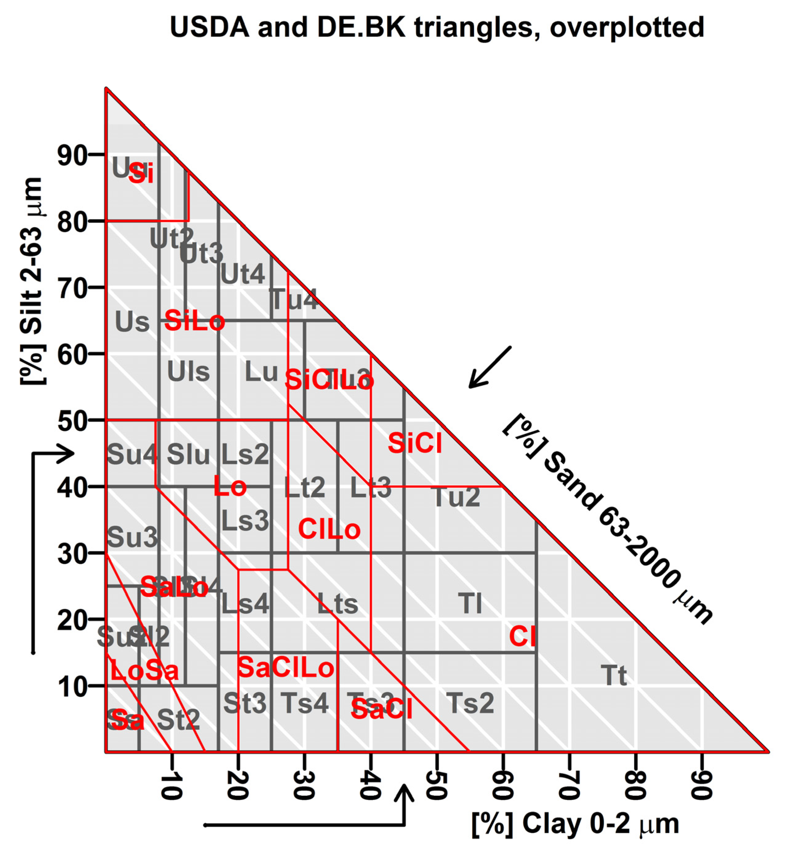
2.2.3. Soil Parameterization

The soil parameterization in BROOK90 requires information of matric potential, soil water content at saturation and field capacity, exponent in the Brooks and Corey equation as given by Clapp and Hornberger [40], hydraulic conductivity at field capacity, and wetness at the dry end of the near-saturation range for a soil layer for each layer of a soil profile. This soil information for whole Saxony can be derived from the BK50 with a 50 m resolution. The BK50 contains specific properties for each soil types, which are classified into 31 soil classes (Figure 2, in black) based on the soil textural properties (percentage of sand, loam, and clay), according to soil science mapping guide (Bodenkundlichen Kartieranleitung, version 5, table 76) [45]. In Saxony, the BK50 in total encloses approximately 1000 soil profiles. They are extended to a maximum of 2.7 m soil depth, if not limited by bedrock.

BK50’s physical properties of soil (bulk density, soil textures of sandy loam and clay) with the help of pedotransfer, can be used to describe soil hydraulic properties, such as soil water retention and hydraulic conductivity functions [3,46]. As suggested by Federer et al. [38], the Clapp and Hornberger hydraulic parameters [40] were applied to describe water movement in soils. However, the parameters sets are available for 12 different soil types (Figure 2, in red), classified according to the American system, USDA [47]. To take advantage of these detailed soil parametrization, we translated the 31 BK50 soil types of the German system into 12 USDA ones using soil texture information, particularly the percentage of sand, silt and clay provided in the associated table of the BK50 (Figure 2). Details can be found in the documentation of the R-package “soiltexture” (https://github.com/julienmoeys/soiltexture).

2.2.4. Spatial Realization

The spatial realization of the model is done with hydro response units (HRUs), also known as hydrotopes. An HRU is defined as a unique combination of topography, land cover, and soil profile. The characteristics required for model parametrization are derived from a 10 m digital elevation model (DEM) and a digitalized soil map at 50 m resolution (BK50), which are provided by LfULG (Sächsisches Landesamt für Umwelt, Landwirtschaft und Geologie, Datenportal für Sachsen), as well as a land cover map at 100 m resolution (CORINE 2012). Fixed parameters were set with default values, as suggested by Federer et al. [38].

HRUs are defined by uniform areas within the catchment according to soil and land-use via superposition. As a result, the Free State of Saxony is split into 115578 HRUs with areas ranging from 2.53 × 10⁻¹⁰ km² to 31 km² (median value at 0.037 km²). Water balance processes are simulated at the HRU scale for all catchments meaning: Each HRU is considered a homogeneous area that allows a plot-scale simulation. BR90-R is thus run for each HRU to estimate water fluxes. The area-weighted average of all HRUs inside the catchment border estimates the final catchment fluxes. Small catchments can already contain up to 100 HRUs or more depending on their location and the resolution of the underlying information of land use and soil. A high number of HRUs considers the variability of the land surface in a catchment; however, this requires high computational effort to use in models.

Since the scope of the study is to represent the water balance on a small to medium catchment scale, Saxony was simulated based on catchments with areas ranging from 0.001 to 115 km² (with a median value of 3 km²). LfULG provides the shapefiles of all 6175 catchments in Saxony. Border catchments with the German States Bavaria, Thuringia, Saxony-Anhalt, and Brandenburg, as well as the Czech Republic or Poland, are included in the simulations only if a minimum of 75% of the area is within the territory of Saxony. In these cases, the external area is not considered in the model and the information from within Saxony is used as a representative for the whole catchment. This setup is due to data availability, which is “State-based” within Germany.

An example of the described approach is given with the Niedermuelsen catchment, as shown in Figure 3. The simplified land use map (b) was intersected with the transformed soil map (c) to derive the combination of HRUs (d). Thus, approximately 500 HRUs are found in the area of 50 km² within the catchment.

Note that the model structure does not allow water exchange between the HRUs, thus, no water flow (routing) within a catchment. The modeling is not fully distributed, but a rather pseudo-spatial representation of water balance components for a catchment. Furthermore, the groundwater recharge process associated with flow parameters in the model is not considered in this study. The evaluation of bypass flow and groundwater flows to the model performance, which requires a systematic calibration, is worth to be a topic on its own. Thus, we focus on an uncalibrated model approach to evaluate the performance of the physically-based parameters. In addition, the meteorological data input is generated for the catchment only, not for each HRU.

2.2.5. Meteorological Data Input

BR90-R requires meteorological measurement information as data input. This data is obtained from the web-based information system described in Wiemann [48], which was developed as part of the EXTRUSO project (https://extruso.bu.tu-dresden.de) at TU Dresden. The platform automatically retrieves and integrates data from various in-situ sensor networks on an hourly basis. This data can be subsequently accessed, processed and downloaded, e.g., for a certain study site. For the area of Saxony, data from more than 2000 hydrological and meteorological sensors are made available. The R-based xtruso package (https://github.com/GeoinformationSystems/xtruso_R) was developed to facilitate the integration of this data for meteorological and hydrological modeling. By using this package in combination with the aforementioned sensor information system, input for the BROOK90 model is generated as follows:

• Selection of a catchment by using catchment ID number integrated with the package;
• Automated extraction of relevant catchment information, i.e., elevation, soil profiles and land covers;
• Automated search for in-situ measurement stations in the surrounding of the catchment (maximum ten stations with a maximum height difference of 200 m to avoid elevation effects);
• Automated extraction and daily aggregation of measurement time series for the identified in-situ stations.

The final input values at the catchment location are estimated from the surrounding measurements by the inverse distance weighting method, widely applied for interpolating climate variables [49,50,51]. The model input requirements are fulfilled by the following daily statistics:

• Mean global radiation;
• Maximum/minimum temperature;
• Mean vapor pressure deficit derived from the mean temperature and the mean relative humidity based on the Magnus equation;
• Mean wind speed; and
• Precipitation sum.

The generated time series serve as data input for all HRUs of the corresponding catchment.

2.3. Model Application and Validation

2.3.1. Model Applicability Test

Implementing the model approach for the whole Free State of Saxony requires a lot of computational time and effort. Each catchment simulation will use the automatic retrieval of meteorological data input, making the simulation of the whole region very time-consuming, even though a parallel mode was integrated into the code. To reduce time, we did a pre-screening of the region by applying the same meteorological data input for six years to all HRUs to test the general possibility of spatial water balance simulation. As a result, around 80% of the area of Saxony was able to be simulated (Figure 4, green color). In particular, this area covers the catchments in the mountainous areas, which have more flooding potential and are where it is difficult to acquire the water fluxes in high resolution. The model did not work for the remaining 20% (also presented in Figure 4). Most errors are caused by translating soil profiles from BK50 into BR90-R (black color). Another error was associated in areas with shallow soil in the upper layers (brown color). During periods of drought, the simulated amount of ET will exceed the simulated amount of water contained in the soil, which will cause the model to stop. Urban areas (red color) are too heterogeneous to model for BR90-R; thus, no reliable parameters are available for this category of land cover. Finally, areas of large water bodies such as rivers, lakes or reservoirs (blue color) are not considered as the BK50 does not provide any soil profile information in these areas.

2.3.2. Validation

The calibration of parameters was not the scope of this paper since we were interested in the raw results of using meaningful physical parameters in BR90-R. Thus, the model performance was directly evaluated against Q, ET, as well as SM data at different spatial and temporal resolutions. The simulation period is 2005–2019, which resulted from a limitation caused by the platform’s data storage capacity. Note that evaluating the model outputs requires excluding a three-month spin up period at the start of each BROOK90 model run to allow the SM to reach a point of equilibrium to avoid its effect on hydrological processes.

A.

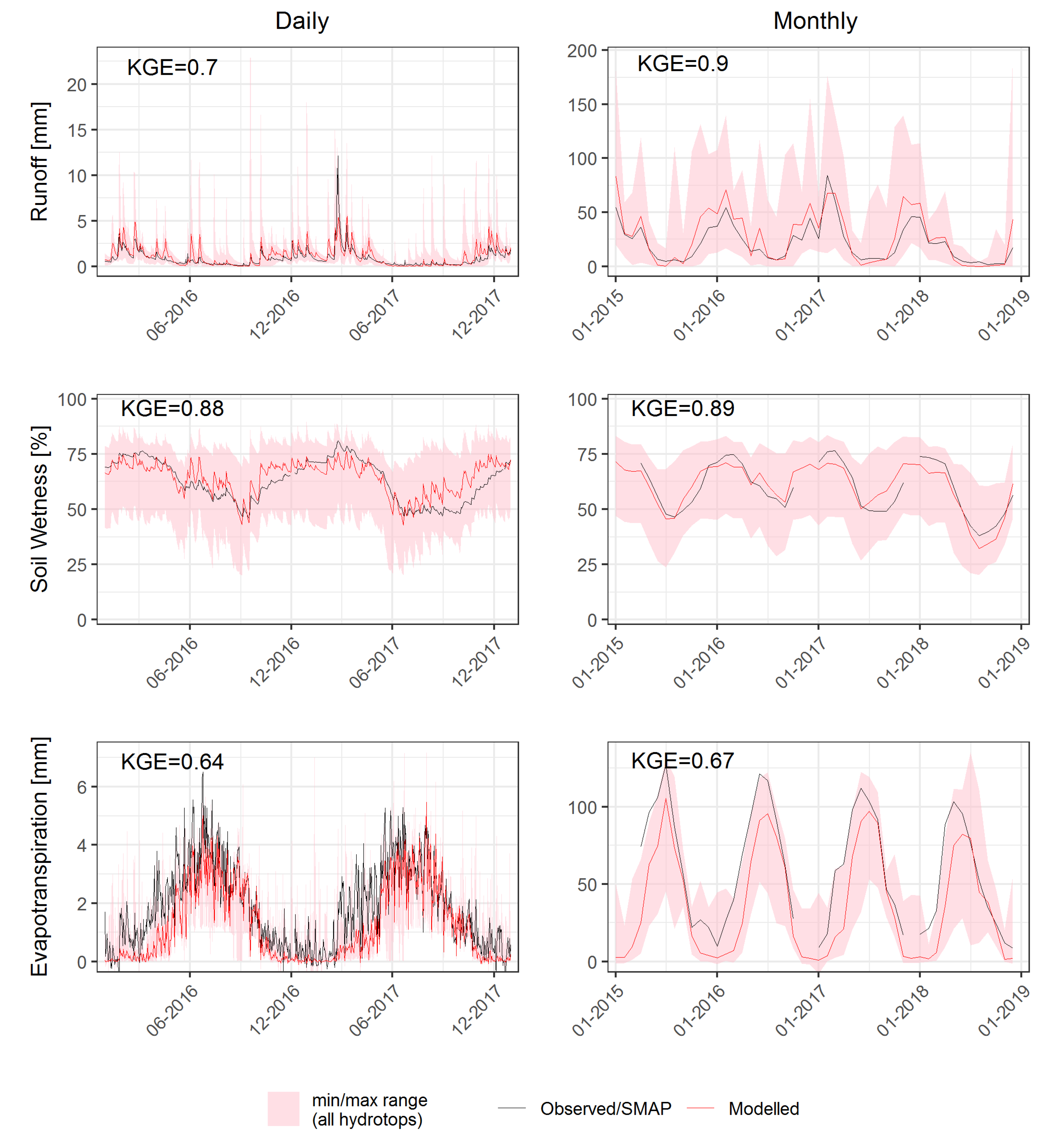
Q: simulated Q was compared with daily and monthly time series of data from flow gauges for the whole simulation period of 2005–2019. The observed Q data for the selected catchments is available in an hourly resolution and unit m³/s provided by LfULG. To use the data in BR90-R, all values were converted to mm/d by considering the catchment area and aggregating Q to daily values.

B.

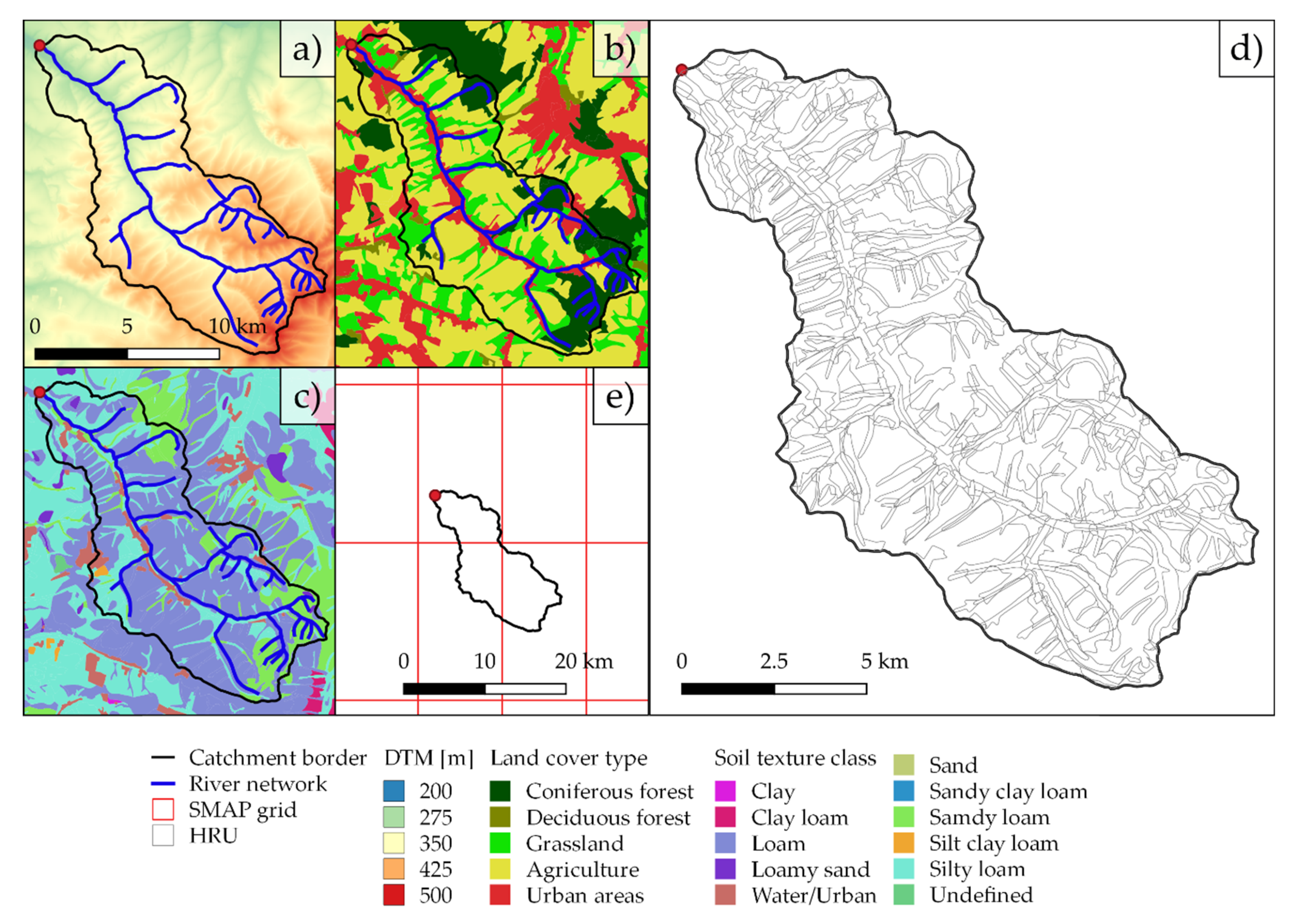
ET: since observed ET from direct measurements is not spatially available in general, we chose to take data from the satellite-based SMAP product, which is based on the Catchment land surface model (LSM) of the NASA Goddard Earth Observing System version 5 (GEOS-5) modeling and assimilation framework [20,52]. ET is taken from SMAP’s Level 4 surface and root-zone soil moisture product (SMAP_L4_GPH) with a spatiotemporal resolution of 9 km × 9 km and 3 hour intervals [20,21]. An illustration of SMAP_L4_GPH grid cells with the example of the Niedermülsen catchment can be seen in Figure 3e. ET data of the product was extracted from all grid cells that are partly or fully covering the considered catchment, area-weighted averages applied and aggregated to daily resolution for validation. Due to data availability, the validation period for ET was chosen from April 2015 to 2018.

C.

SM: SM data were retrieved from SMAP_L4_GPH similar to ET with the following additional step: SM from BR90-R was divided into the soil profile porosity (BK50) to derive SM wetness, which is comparable with SM from SMAP. The same validation period as ET was chosen. Note that both described, SM and ET are not considered true observations, rather additional sources to cross-check the model performance. Still, both assimilated values are based on observations by the satellite.

As commonly done in hydrological research and other disciplines [22,53], the skill score Kling–Gupta efficiency (KGE) [54] and its decomposition components (correlation, mean bias, and variability bias) were chosen to quantify the model results with the following Equation (1):

$$KGE=1-\sqrt{{\left(R-1\right)}^2+{\left(\alpha -1\right)}^2+{\left(\beta -1\right)}^2}$$

(1)

With R being the correlation coefficient, $\alpha ={\sigma }_{sim}/{\sigma }_{obs}$ the standard deviations $\sigma$ of simulations and observations, and $\beta ={\mu }_{sim}/{\mu }_{obs}$ being the ratio of the simulated and observed means $\mu$. KGE will equal 1 for a perfect fit of the simulation when R, $\alpha$ and $\beta$ are all at their optimal value 1. One of the advantages of using KGE is the consideration of multiple aspects in the comparison. However, according to [55], the KGE value at-0.41 shows that the model performance is as good as the observed mean flow.

3. Results and Discussions

3.1. Variation between HRUs

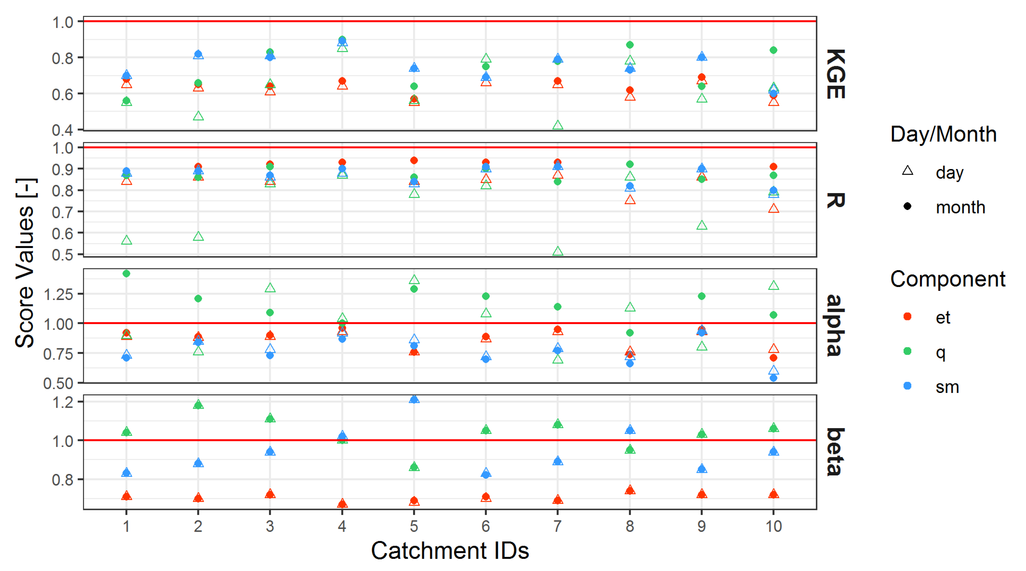
The comparison of simulated and observed water balance components are shown with the example of Krummenhennersdorf catchment in Figure 5.

Figures for other catchments can be found in the Supplementary Materials. For a better display, daily values (left column) are shown from January 2015 to December 2016 (2 years), and monthly values (right column) are shown from January 2015 to December 2018. Modeled and observed Q values matched well on the seasonal dynamics of water flow, namely high Q in the spring months due to snowmelt and low in summer months due to the high rate of ET. Generally, good agreements are seen in both temporal scales. Particularly, the long duration of low flow conditions in the year 2018 (and, not shown in Figure 5: 2019) due to the drought situation in Germany was captured well. The simulated peak flows are overestimated on a daily scale; however, they are improved on a monthly scale. The seasonal pattern of SM and ET are visible on daily and monthly scales with wet soils in winter months and dry soils in summer months, as a consequence of ET response to inter-annual radiation pattern. This behavior was observed in all selected catchments. Interestingly, the drought from 2018 (whole Germany) via SM was clearly shown in the simulation results.

Generally, the selected catchments show no distinct difference in the behavior of the water components itself since they are located in the same climate zone. Within one catchment, there is a large range between minimum and maximum values of the corresponding hydrotopes for all water balance components, indicating the great variety of possible catchment responses. Due to the general higher variability of flow values, the range of simulated discharge values is higher than for ET and SM. From the first impression, it seems that the average values of simulated SM especially fits well with the SMAP observations and that there is a good representation of the ET pattern while the ET values of SMAP seem to be a bit replaced, especially for summer months. One interesting observation was that the range of SM values between the HRUs is similarly high for all catchments, independent of their area sizes. These variations show the high spatial heterogeneity of SM and, thus, emphasizes the importance of representing SM at a high resolution [16,56].

3.2. Skill Score

3.2.1. Catchments Average

In this section, we present a quantitative evaluation via selected skill scores for simulated water balance components. The area-weighted mean values of the considered variables Q, SM, and ET (red lines in Figure 5) were used as representatives for the catchments for comparing the simulations with observations. The mean values of the skill scores for all ten catchments are displayed in

Table 3. Average skill score of all catchments (KGE: Kling Gupta efficiency, R: Pearson correlation, $\alpha$: standard deviation ratio, $\beta$ mean ratio between BROOK90 model outputs and “observation”) for discharge (Q), SM and ET.

Variable	Validation Period	Daily Resolution				Monthly Resolution
		KGE	R	$\mathit{\alpha }$	$\mathit{\beta }$	KGE	R	$\mathit{\alpha }$	$\mathit{\beta }$
Mean Q	2005–2019	0.63	0.72	1.04	1.04	0.75	0.88	1.16	1.04
Mean SM	2015–2018	0.76	0.86	0.79	0.94	0.76	0.87	0.76	0.94
Mean ET	2015–2018	0.62	0.83	0.86	0.70	0.65	0.92	0.87	0.71

. On a daily scale, the mean values for daily Q are 0.63 (KGE), 0.72 (R), 1.04 and 1.04 (ratios of standard deviation ($\alpha$) respectively mean ($\beta$)), which indicate an acceptable performance of the model. A slight improvement of the Q simulation was observed on a monthly scale (0.75 (KGE), 0.88 (R), 1.16 and 1.04 ($\alpha$ and $\beta$)). While high values of KGE and R confirm a good performance of the model approach, the values of $\alpha$ and $\beta$ greater than one shows an overall overestimation of Q. This issue is likely caused by excluding bypass flow and groundwater recharge processes from the simulation. Thus, water, which is lost to an aquifer, is eventually accumulated at the catchment outlet. A similar conclusion was drawn by Vorobevskii et al. [30], which also applied a similar approach.

The skill scores of SM between the two datasets of BR90-R and LSM from SMAP products show an overall good correspondence on a daily scale and a monthly scale. The values for both scales are almost identical. High KGE (KGE > 0.75) and correlation (R > 0.85) was observed in the validation period. However, $\alpha$ (<0.8) and $\beta$ (=0.94) indicate, in general, an underestimation of soil wetness derived from BR90-R compared to LSM. This result arises because of the differences in the model setups, e.g., due to model structure, data input, land cover map, soil map, parameterization approach as well as resolution. Additionally, the pedotransfer function applied in the LSM was derived from Wösten et al. [46] and updated by De Lannoy et al. [57], which has a different approach compared to the Br90-R [38]. Last but not least, the non-representative of 9 km × 9 km model grid cell of SMAP for the area-weighted mean of the HRUs approach can be accountable for this underestimation.

Similarto the SM results, the skill scores of ET for the two products show a good agreement on both scales. While KGE > 0.6 and R > 0.8 exhibits a relatively good correlation of ET, $\alpha$ = 0.86 and $\beta$ = 0.70 indicate the underestimation of ET from the BR90-R compared to ET from LSM. Even though both models use the Penman-Monteith equation [58] to describe ET processes, approximately 20% of ET of the BR90-R was less than the one from LSM, which is due to the abovementioned reasons relating to the model setups and miscalling issue.

More detail can be seen in the analyses for individual catchment and seasonal variability in the next section.

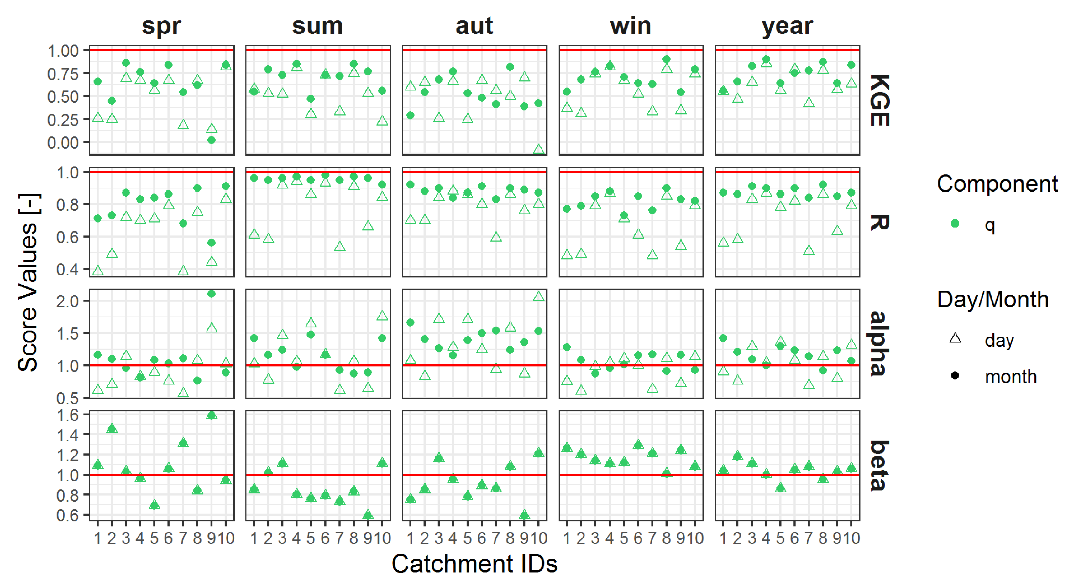
3.2.2. Catchment and Seasonal Variation

The evaluation based on skill cores for the simulations and observations varied from catchment to catchment as well as to water balance components (Figure 6). Note that the catchment names can be found via catchment IDs in Table 1. Overall, the water balance components dynamics of ten selected catchments are satisfactorily captured by the model in the study period. The ranges of KGEs for Q corresponding to the ten selected catchments are 0.42 to 0.85 on a daily scale and 0.56 to 0.9 on a monthly scale. The spread of KGEs for the monthly Q is slightly narrower compared to daily flows. This pattern is also applied to R and $\alpha$ values. As expected, the high temporal variability of daily Q is flattened when averaging over a longer (monthly) period, which leads to an overall better agreement between observed and simulated Q. The best model performances were found at Krummenhennersdorf (KGE > 0.85) and Niederzwoenitz (KGE > 0.78), where the differences between daily scale and monthly were minor. A relatively lower model skill in simulating the Q dynamics was observed at Grossschweidnitz, Holtendorf, Niederoderwitz, and Reichenbach Oberlausitz (numbers 1, 2, 7, and 9 in Figure 1 and Figure 6), which are located at the farthest East from Saxony, namely the Oberlausitz region. These results could be attributed to the lack of information on meteorological data input due to a sparse network of sensor measurements. Additionally, sensors data from the neighboring countries, such as the Czech Republic and Poland, are not available, thus, not integrated into this study. Nevertheless, the model performances of the four abovementioned catchments are considered acceptable comparing to those found by previous studies, such as [30,37,59]. Thus, we conclude that the uncalibrated version of the BROOK90 model can capture the Q dynamics in the ten selected catchments.

In addition, evaluating the skill scores for SM and ET between the BR90-R model and the LSM in the study period confirms a good correspondence in all catchments. The ranges of KGEs are 0.6 to 0.89 and 0.55 to 0.69 for SM and ET, respectively (Figure 6). Unlike the Q dynamics, the model performances of SM and ET were consistent on both scales in all catchments. A clear pattern can be observed is that SM and ET from the BR90-R were estimated as lower than from the LSM reveal by the ranges of $\alpha$ (0.54 to 0.94 for SM and 0.71 to 0.96 for ET) and the ranges of $\beta$ (0.82 to 1.21 for SM and 0.67 to 0.74 for ET). An exception was found at the catchment Neustadt (number 5 in Figure 1 and Figure 6), where soil wetness derived from the BR90-R is wetter than the LSM. This could be attributed to the soil profiles derived from the two maps applied in the models, which accidentally caused the overestimation of SM in the catchment. We observed further the relationships between model performance and the characteristics of the selected catchments (e.g., topography, land cover, area, as well as the density of HRUs, as listed in Table 1). We could not see any correlation. In contrast, the studies of Newman et al. [60] or Mc Millan et al. [61] exhibited a clear dependency between model performance to characteristics, such as the catchment area. Thus, the observation from the ten catchments might suggest the validity of the approach for the regional scale.

The model simulations were further evaluated for the seasonal variability as our study sites are located in a temperate region, which is significantly characterized by seasons. We considered only Q and estimated the selected skill scores in the study period on both daily and monthly scales (Figure 7). The average KGEs on a monthly scale of ten selected catchments is 0.62, 0.70, 0.53, and 0.70 for spring, summer, autumn, and winter, respectively. The highest variation in terms of $\beta$ (0.6 to 1.6) was observed during spring, when the snowmelt process takes place, and the lowest in winter, in which the loss of ET is lowest among seasons. In addition, we observed very high and consistent correlations in all catchments on a monthly scale in summer, although most of the high precipitation events due to convective rainfall occur during this time. Hence, we can assume that the sensor measurements from the platform can capture such events well. Last, but not least, the consistent values of $\alpha$ and $\beta$ values reveal outperformance in winter comparing to other seasons. This can be attributed to saturated SM in winter, which supports surface flow processes quickly after a rainfall event. Thus, the impact of the infiltration process is reduced, and the model can well capture the Q dynamics.

4. Conclusions and Outlook

In this study, we present a new approach to simulate water balance components at a high spatial resolution using the BROOK90 model integrated into the data platform developed in the EXTRUSO project. The model is not calibrated and its parameters are derived merely by detailed orographic, land use, and soil information, as well as available literature. It is feasible as most of the parameters of the model have physical meanings, which can be measured and/or transferred from similar study sites. The simulations were followed by the HRU approach and applicable for more than 80% area of Saxony. The validation in ten selected head catchments in a low mountain range showed a reliable model performance. Thus, our results underline that the automatic parametrization approach performed assuredly with available information in the study site. Additionally, the uncalibrated model version revealed itself to be able to deliver reasonably distributed water balance components. The study provides a feasible way to consider the changing climate conditions and shows that a physically-based lumped model can substitute for a spatially distributed one on a regional scale. Nevertheless, numerous drawbacks are resulting from the model structure, parameterization approach, modeling concept, and validation data, which will be considered in our ongoing work.

• The lack of routing mode in the model structure causes the estimation of the discharge to be mere as the water remaining after ET, SM, and groundwater processes. Thus, the simulated Q has rather a meaning of an amount of accumulated water than its temporal distribution characteristics [2]. It can be seen at the daily scale of the validation of the ten catchments. Integrating an additional routing mode may solve this problem and would approach fully distributed. It can be implemented as the BR90-R version allows for coupling external modules in its structure; however, this step can cause more computational time and loosen the characteristics of HRUs.
• The evaluation regarding discharge for individual catchments revealed an uncertainty of the model performance in the border region, namely the Oberlausitz at the farthest east of the state. It may be caused by the limitation of the density of climate stations in the region, which makes it difficult to capture the climate conditions representatively. Thus, a high spatial resolution climate dataset such as precipitation from radar data can overcome this issue.
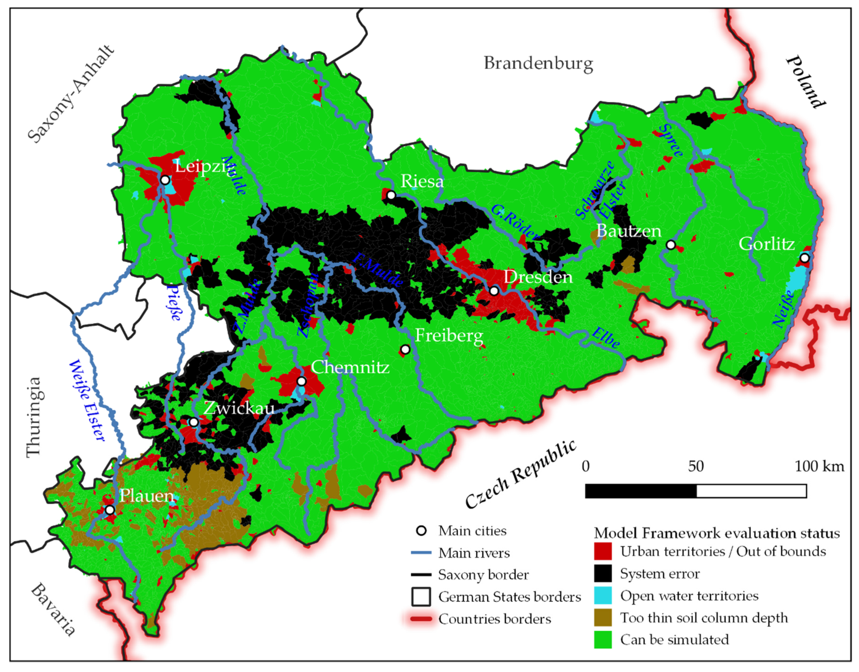
• The 20% areas, where the model cannot be implemented, can be adjusted by modifying the soil profiles. For instance, soils with shallow surface horizons can be fixed by combining several thin layers into one with which we can obtain a new soil profile with similar soil hydraulic properties. For urban areas out of the scope of the application of the model, pre-event SM derivation for an area, the curve number method (also called the Soil Conservation Service or SCS) [62,63,64] can be applied as a good alternative. The areas that caused system errors were found to be associated with lacking soil profile information from the BK50, which prevents the simulation in the sub-soil-process of the model. Thus, an updated, more precise soil map, is needed.
• The suggested approach to derive parameters from the soil and land use maps is a good practice to translate the characteristics of the catchments to the model. Nevertheless, the parameterization is still limited due to the simplification of land cover classes to one species and the transformation of soil systems. A systematic calibration for all of the catchments might improve or compensate for such discrepancies. In other words, a spatial parameter derivation is needed.
• SMAP_L4_GPH is a valuable data source to validate model outputs, particularly at a regional scale. However, a direct comparison with in situ measurements is a better choice to prove the plausibility of the ET and SM.

References

1. Zink, M.; Kumar, R.; Cuntz, M.; Samaniego, L. A high-resolution dataset of water fluxes and states for Germany accounting for parametric uncertainty. Hydrol. Earth Syst. Sci. 2017, 21, 1769–1790. [Google Scholar] [CrossRef] [Green Version]
2. Schwärzel, K.; Feger, K.-H.; Häntzschel, J.; Menzer, A.; Spank, U.; Clausnitzer, F.; Köstner, B.; Bernhofer, C. A novel approach in model-based mapping of soil water conditions at forest sites. For. Ecol. Manag. 2009, 258, 2163–2174. [Google Scholar] [CrossRef]
3. Schmidt-Walter, P.; Ahrends, B.; Mette, T.; Puhlmann, H.; Meesenburg, H. NFIWADS: The water budget, soil moisture, and drought stress indicator database for the German National Forest Inventory (NFI). Ann. For. Sci. 2019, 76. [Google Scholar] [CrossRef] [Green Version]
4. Penna, D.; Tromp-Van Meerveld, H.J.; Gobbi, A.; Borga, M.; Dalla Fontana, G. The influence of soil moisture on threshold runoff generation processes in an alpine headwater catchment. Hydrol. Earth Syst. Sci. 2011, 15, 689–702. [Google Scholar] [CrossRef] [Green Version]
5. Brocca, L.; Ciabatta, L.; Massari, C.; Camici, S.; Tarpanelli, A. Soil moisture for hydrological applications: Open questions and new opportunities. Water 2017, 9, 140. [Google Scholar] [CrossRef]
6. Kumar, R.; Musuuza, J.L.; Van Loon, A.F.; Teuling, A.J.; Barthel, R.; Ten Broek, J.; Mai, J.; Samaniego, L.; Attinger, S. Multiscale evaluation of the Standardized Precipitation Index as a groundwater drought indicator. Hydrol. Earth Syst. Sci. 2016, 20, 1117–1131. [Google Scholar] [CrossRef] [Green Version]
7. Samaniego, L.; Kumar, R.; Zink, M. Implications of Parameter Uncertainty on Soil Moisture Drought Analysis in Germany. Am. Meteorol. Soc. 2013, 47–68. [Google Scholar] [CrossRef]
8. Sheffield, J.; Goteti, G.; Wen, F.; Wood, E.F. A simulated soil moisture based drought analysis for the United States. J. Geophys. Res. D Atmos. 2004, 109, 1–19. [Google Scholar] [CrossRef]
9. Hanel, M.; Rakovec, O.; Markonis, Y.; Máca, P.; Samaniego, L.; Kyselý, J.; Kumar, R. Revisiting the recent European droughts from a long-term perspective. Sci. Rep. 2018, 8, 9499. [Google Scholar] [CrossRef]
10. European Environment Agency. Meteorological and Hydrological Droughts; European Environment Agency: Copenhagen, Denmark, 2019; p. 13. [Google Scholar]
11. Ashley, R.M.; Blanksby, J.R.; Cashman, A. A methodology for adapting local drainage to climate change. In Flood Risk Management: Research and Practice; Taylor & Francis Group: London, UK, 2010; pp. 301–302. ISBN 978-0-415-48507-4. [Google Scholar]
12. te Linde, A.H.; Aerts, J.C.J.H. Simulating flood-peak probability in the Rhine basin and the effect of climate change. In Flood Risk Management: Research and Practice; Taylor & Francis Group: London, UK, 2008; pp. 1729–1736. ISBN 978-0-415-48507-4. [Google Scholar]
13. Vereecken, H.; Huisman, J.A.; Bogena, H.; Vanderborght, J.; Vrugt, J.A.; Hopmans, J.W. On the value of soil moisture measurements in vadose zone hydrology: A review. Water Resour. Res. 2008, 46, 1–21. [Google Scholar] [CrossRef] [Green Version]
14. Entekhabi, D.; Das, N.; Njoku, E.; Yueh, S.; Johnson, J.; Shi, J. Soil Moisture Active Passive (SMAP) Algorithm Theoretical Basis Document L2 & L3 Radar/Radiometer Soil Moisture (Active/Passive) Data Products Table of Contents; California Institute of Technology: Pasadena, CA, USA, 2014. [Google Scholar]
15. Dorigo, W.A.; Wagner, W.; Hohensinn, R.; Hahn, S.; Paulik, C.; Drusch, M.; Mecklenburg, S.; van Oevelen, P.; Robock, A.; Jackson, T. The International Soil Moisture Network: A data hosting facility for global in situ soil moisture measurements. Hydrol. Earth Syst. Sci. Discuss. 2011, 8, 1609–1663. [Google Scholar] [CrossRef]
16. Rinderer, M.; Seibert, J. Soil Information in Hydrologic Models: Hard Data, Soft Data, and the Dialog between Experimentalists and Modelers. Hydropedology 2012, 515–536. [Google Scholar] [CrossRef]
17. Falge, E.; Aubinet, M.; Bakwin, P.S.; Baldocchi, D.; Berbigier, P.; Bernhofer, C.; Black, T.A.; Ceulemans, R.; Davis, K.J.; Dolman, A.J.; et al. FLUXNET Research Network Site Characteristics, Investigators, and Bibliography, 2016; ORNL Distributed Active Archive Center, ORNL DAAC: Oak Ridge, TN, USA, 2017. [CrossRef]
18. Brocca, L.; Melone, F.; Moramarco, T.; Wagner, W.; Naeimi, V.; Bartalis, Z.; Hasenauer, S. Improving runoff prediction through the assimilation of the ASCAT soil moisture product. Hydrol. Earth Syst. Sci. 2010, 14, 1881–1893. [Google Scholar] [CrossRef] [Green Version]
19. Naz, B.S.; Kurtz, W.; Montzka, C.; Sharples, W.; Goergen, K.; Keune, J.; Gao, H.; Springer, A.; Kollet, S. Improving soil moisture and runoff simulations at 3&km over Europe using land surface data assimilation. Hydrol. Earth Syst. Sci. 2019, 23, 277–301. [Google Scholar] [CrossRef] [Green Version]
20. Reichle, R.H.; De Lannoy, G.J.M.; Liu, Q.; Koster, R.D.; Kimball, J.S.; Crow, W.T.; Ardizzone, J.V.; Chakraborty, P.; Collins, D.W.; Conaty, A.L.; et al. Global Assessment of the SMAP Level-4 Surface and Root-Zone Soil Moisture Product Using Assimilation Diagnostics. J. Hydrometeorol. 2017, 18, 3217–3237. [Google Scholar] [CrossRef]
21. Reichle, R.H.; Liu, Q.; Koster, R.D.; Crow, W.T.; De Lannoy, G.J.M.; Kimball, J.S.; Ardizzone, J.V.; Bosch, D.; Colliander, A.; Cosh, M.; et al. Version 4 of the SMAP Level-4 Soil Moisture Algorithm and Data Product. J. Adv. Model. Earth Syst. 2019, 11, 3106–3130. [Google Scholar] [CrossRef] [Green Version]
22. Lievens, H.; Tomer, S.K.; Al Bitar, A.; De Lannoy, G.J.M.; Drusch, M.; Dumedah, G.; Hendricks Franssen, H.J.; Kerr, Y.H.; Martens, B.; Pan, M.; et al. SMOS soil moisture assimilation for improved hydrologic simulation in the Murray Darling Basin, Australia. Remote Sens. Environ. 2015, 168, 146–162. [Google Scholar] [CrossRef]
23. Xu, Y.; Wang, L.; Ross, K.W.; Liu, C.; Berry, K. Standardized soil moisture index for drought monitoring based on soil moisture active passive observations and 36 years of North American Land Data Assimilation System data: A case study in the Southeast United States. Remote Sens. 2018, 10, 301. [Google Scholar] [CrossRef] [Green Version]
24. Bai, J.; Cui, Q.; Chen, D.; Yu, H.; Mao, X.; Meng, L.; Cai, Y. Assessment of the SMAP-Derived Soil Water Deficit Index (SWDI-SMAP) as an Agricultural Drought Index in China. Remote Sens. 2018, 10, 1302. [Google Scholar] [CrossRef] [Green Version]
25. Matgen, P.; Fenicia, F.; Heitz, S.; Plaza, D.; de Keyser, R.; Pauwels, V.R.N.; Wagner, W.; Savenije, H. Can ASCAT-derived soil wetness indices reduce predictive uncertainty in well-gauged areas? A comparison with in situ observed soil moisture in an assimilation application. Adv. Water Resour. 2012, 44, 49–65. [Google Scholar] [CrossRef]
26. Escorihuela, M.J.; Quintana-seguí, P. Remote Sensing of Environment Comparison of remote sensing and simulated soil moisture datasets in Mediterranean landscapes. Remote Sens. Environ. 2016, 180, 99–114. [Google Scholar] [CrossRef] [Green Version]
27. Yu, P.; Wang, Y.; Du, A.; Guan, W.; Feger, K.H.; Schwärzel, K.; Bonell, M.; Xiong, W.; Pan, S. The effect of site conditions on flow after forestation in a dryland region of China. Agric. For. Meteorol. 2013, 178–179, 66–74. [Google Scholar] [CrossRef]
28. Peters, R.; Clausnitzer, F.; Köstner, B.; Bernhofer, C.; Feger, K.H.; Schwärzel, K. Einfluss von Boden und Bestockung auf den Standortswasserhaushalt. Wald. Online 2011, 12, 101–109. [Google Scholar]
29. Spank, U.; Schwärzel, K.; Renner, M.; Moderow, U.; Bernhofer, C. Effects of measurement uncertainties of meteorological data on estimates of site water balance components. J. Hydrol. 2013, 492, 176–189. [Google Scholar] [CrossRef]
30. Vorobevskii, I.; Kronenberg, R.; Bernhofer, C. Global BROOK90 (R-package): An automatic framework to simulate the water balance at any location. Water 2020, 12, 2037. [Google Scholar] [CrossRef]
31. Wiemann, S.; Eltner, A.; Sardemann, H.; Spieler, D.; Singer, T.; Thanh, T. On the monitoring and prediction of flash floods in small and medium-sized catchments—The EXTRUSO project. In Proceedings of the 19th EGU General Assembly, EGU2017, Vienna, Austria, 23–28 April 2017; p. 4862. [Google Scholar]
32. Blöschl, G. Rainfall-Runoff Modeling of Ungauged Catchments. Encycl. Hydrol. Sci. 2005. [Google Scholar] [CrossRef]
33. LfULG. Sachsen im Klimawandel; Staatsministerium fuer Umwelt und Landwirtschaft: Saxony, Germany, 2019. [Google Scholar]
34. Schwarze, R.; Gurova, A.; Röhm, P.; Hauffe, C. Wasserhaushalt im Wandel von Klima und Landnutzung. Schriftenreihe LfULG; Landesamt fuer Umwelt, Landwirtschaft und Geologie: Saxony, Germany, 2016; p. 139. [Google Scholar]
35. Petzold, R.; Burse, K.; Benning, R.; Gemballa, R. Die Lokalbodenform im System der forstlichen Standortserkundung im Mittelgebirge/Hügelland und deren bodenphysikalischer Informationsgehalt. Wald. Landsch. Nat. For. Ecol. Landsc. Res. Nat. Conserv. 2016, 16, 29–33. [Google Scholar]
36. Benning, R.; Petzold, R.; Danigel, J.; Gemballa, R.; Andreae, H. Generating characteristic soil profiles for the plots of the National Forest Inventory in Saxony and Thuringia. Wald. Landsch. Nat. For. Ecol. Landsc. Res. Nat. Conserv. 2016, 16, 35–42. [Google Scholar]
37. Gebrechorkos, S.H.; Bernhofer, C.; Hülsmann, S. Impacts of projected change in climate on water balance in basins of East Africa. Sci. Total Environ. 2019, 682, 160–170. [Google Scholar] [CrossRef]
38. Federer, C.A.; Vörösmarty, C.; Fekete, B. Sensitivity of Annual Evaporation to Soil and Root Properties in Two Models of Contrasting Complexity. J. Hydrometeorol. 2003, 4, 1276–1290. [Google Scholar] [CrossRef]
39. Campbell, G.S. A simple method for determining unsaturated conductivity from moisture retention data. Soil Sci. 1974, 117, 311–314. [Google Scholar] [CrossRef]
40. Clapp, R.B.; Hornberger, G.M. Empirical equations for some soil hydraulic properties. Water Resour. Res. 1978, 14, 601–604. [Google Scholar] [CrossRef] [Green Version]
41. Bonan, G.B.; Levis, S.; Kergoat, L.; Oleson, K.W. Landscapes as patches of plant functional types: An integrating concept for climate and ecosystem models. Glob. Biogeochem. Cycles 2002, 16, 5-1–5-23. [Google Scholar] [CrossRef] [Green Version]
42. Petzold, R.; Danigel, J.; Benning, R.; Mayer, S.; Burse, K.; Karas, F.; Andreae, H.; Gemballa, R. Aus Alt mach Neu—Altdaten der Standortskartierung für die räumlich differenzierte Ableitung der Bodenwasserspeicherung of water storage pro. Wald. Landsch. Nat. For. Ecol. Landsc. Res. Nat. Conserv. 2016, 16, 19–27. [Google Scholar]
43. Bernhofer, C.; Grünwald, T.; Spank, U.; Clausnitzer, F.; Eichelmann, U.; Köstner, B.; Prasse, H.; Feger, K.H.; Menzer, A.; Schwärzel, K. Mikrometeorologische, pflanzenökologische und bodenhydrologische messungen in fichten- und buchenbeständen des tharandter waldes. Wald. Online 2011, 12, 17–28. [Google Scholar]
44. Schwärzel, K.; Menzer, A.; Clausnitzer, F.; Spank, U.; Häntzschel, J.; Grünwald, T.; Köstner, B.; Bernhofer, C.; Feger, K.H. Soil water content measurements deliver reliable estimates of water fluxes: A comparative study in a beech and a spruce stand in the Tharandt forest (Saxony, Germany). Agric. For. Meteorol. 2009, 149, 1994–2006. [Google Scholar] [CrossRef]
45. Eckelmann, W.; Sponagel, H.; Grottenthaler, W.; Hartmann, K.-J.; Hartwich, R.; Janetzko, P.; Joisten, H.; Kühn, D.; Sabel, K.-J.; Traidl, R. AD-HOC-Arbeitsgruppe Boden der Staatlichen Geologischen Dienste der Bundesanstalt für Geowissenschaften und Rohstoffe; Schweizerbart Science Publishers: Stuttgart, Germany, 2005; ISBN 9783510959204. [Google Scholar]
46. Wösten, J.H.M.; Pachepsky, Y.A.; Rawls, W.J. Pedotransfer functions: Bridging the gap between available basic soil data and missing soil hydraulic characteristics. J. Hydrol. 2001, 251, 123–150. [Google Scholar] [CrossRef]
47. Canfield, H.E.; Lopes, V.L. Simulating soil moisture change in a semiarid rangeland watershed with a process-based water-balance model. In Proceedings RMRS; USDA Forest Service: Washington, DC, USA, 2000; pp. 316–319. [Google Scholar]
48. Wiemann, S. Beitrag J: Stefan Wiemann Web-Basierte Analyse und Prozessierung hydro-Meteorologischer Daten im Kontext von Extremereignissen (Web-Based Analysis and Processing of Hydro-Meteorological Data in the Context of Extreme Events); Umweltinformationssystem UIS 2018: Nuernberg, Germany, 2018; pp. 139–148. [Google Scholar]
49. Abatzoglou, J.T. Development of gridded surface meteorological data for ecological applications and modelling. Int. J. Climatol. 2013, 33, 121–131. [Google Scholar] [CrossRef]
50. Nusret, D.; Dug, S. Applying the Inverse Distance Weighting and Kriging methods of the spatial interpolation on the mapping the annual precipitation in Bosnia and Herzegovina. In Proceedings of the 6th Biennial Meeting of the International Environmental Modelling and Software Society, Leipzig, Germany, 1 July 2012; pp. 2754–2760. [Google Scholar]
51. Ozelkan, E.; Bagis, S.; Ustundag, B.B.; Yucel, M.; Ozelkan, E.C.; Ormeci, C. Land surface temperature—Based spatial interpolation using a modified inverse distance weighting method. In Proceedings of the 2013 2nd International Conference on Agro-Geoinformatics: Information for Sustainable Agriculture, Agro-Geoinformatics, Washington, DC, USA, 12–16 August 2013; pp. 110–115. [Google Scholar] [CrossRef]
52. Koster, R.D.; Suarez, M.J.; Ducharne, A.; Stieglitz, M.; Kumar, P. A catchment-based approach to modeling land surface processes in a general circulation model: 1. Model structure. J. Geophys. Res. Atmos. 2000, 105, 24809–24822. [Google Scholar] [CrossRef]
53. Cai, X.; Pan, M.; Chaney, N.W.; Colliander, A.; Misra, S.; Cosh, M.H.; Crow, W.T.; Jackson, T.J.; Wood, E.F. Validation of SMAP soil moisture for the SMAPVEX15 field campaign using a hyper-resolution model. Water Resour. Res. 2017, 53, 3013–3028. [Google Scholar] [CrossRef]
54. Gupta, H.V.; Kling, H.; Yilmaz, K.K.; Martinez, G.F. Decomposition of the mean squared error and NSE performance criteria: Implications for improving hydrological modelling. J. Hydrol. 2009, 377, 80–91. [Google Scholar] [CrossRef] [Green Version]
55. Knoben, W.J.M.; Freer, J.E.; Woods, R.A. Technical note: Inherent benchmark or not? Comparing Nash-Sutcliffe and Kling-Gupta efficiency scores. Hydrol. Earth Syst. Sci. 2019, 23, 4323–4331. [Google Scholar] [CrossRef] [Green Version]
56. Staudinger, M.; Stahl, K.; Stoelzle, M.; Seeger, S.; Seibert, J.; Weiler, M. Catchment water storage variation with elevation. Hydrol. Process. 2017, 31, 2000–2015. [Google Scholar] [CrossRef]
57. De Lannoy, G.J.M.; Koster, R.D.; Reichle, R.H.; Mahanama, S.P.P.; Liu, Q. An updated treatment of soil texture and associated hydraulic properties in a global land modeling system. J. Adv. Model. Earth Syst. 2014, 6, 957–979. [Google Scholar] [CrossRef] [Green Version]
58. Allen, R.G.; Pereira, L.S.; Raes, D.; Smith, M. FAO Irrigation and Drainage Paper No. 56, Crop Evapotranspiration (Guidelines for Computing Crop Water Requirements); FAO: Rome, Italy, 1998; 328p. [Google Scholar]
59. Fleischbein, K.; Lindenschmidt, K.; Merz, B. Modelling the runoff response in the Mulde catchment (Germany). In Advances in Geosciences; European Geosciences Union: Munich, Germany, 2006; pp. 79–84. [Google Scholar]
60. Newman, A.J.; Clark, M.P.; Sampson, K.; Wood, A.; Hay, L.E.; Bock, A.; Viger, R.J.; Blodgett, D.; Brekke, L.; Arnold, J.R.; et al. Development of a large-sample watershed-scale hydrometeorological data set for the contiguous USA: Data set characteristics and assessment of regional variability in hydrologic model performance. Hydrol. Earth Syst. Sci. 2015, 19, 209–223. [Google Scholar] [CrossRef] [Green Version]
61. McMillan, H.K.; Booker, D.J.; Cattoën, C. Validation of a national hydrological model. J. Hydrol. 2016, 541, 800–815. [Google Scholar] [CrossRef]
62. Soulis, K.X.; Valiantzas, J.D. SCS-CN parameter determination using rainfall-runoff data in heterogeneous watersheds-the two-CN system approach. Hydrol. Earth Syst. Sci. 2012, 16, 1001–1015. [Google Scholar] [CrossRef] [Green Version]
63. Satheeshkumar, S.; Venkateswaran, S.; Kannan, R. Rainfall–runoff estimation using SCS–CN and GIS approach in the Pappiredipatti watershed of the Vaniyar sub basin, South India. Model. Earth Syst. Environ. 2017, 3, 24. [Google Scholar] [CrossRef]
64. Rozalis, S.; Morin, E.; Yair, Y.; Price, C. Flash flood prediction using an uncalibrated hydrological model and radar rainfall data in a Mediterranean watershed under changing hydrological conditions. J. Hydrol. 2010, 394, 245–255. [Google Scholar] [CrossRef]
Figure 1. An overview of ten selected catchments for validation (WGS-84 Pseudo-Mercator projection) with a background from a digital elevation model (DEM) based on SRTM30. The ID numbers of the catchments can be referred to in Table 1.
Hydrology 07 00084 g001
Figure 2. Over plotted soil types classified after the American system USDA (in red) and the German system (in black). The abbreviations of the soil types in the two systems are well documented in the “soiltexture” package.
Hydrology 07 00084 g002
Figure 3. An overview of the input datasets (WG-S 84 projection), exemplary for the Niedermuelsen catchment: (a) digital elevation model (DEM) based on 10 m, (b) land use map simplified from CORINE 2012, (c) soil map converted from USDA soil classes and simplified from BK50, (d) hydro response units (HRUs): intersecting between simplified CORINE and BK50 and (e) SMAP_L4_GPH grid tiles.
Hydrology 07 00084 g003
Figure 4. Overview of the approach performance in the Free State of Saxony.
Hydrology 07 00084 g004
Figure 5. Daily and monthly time series of simulated (weighted mean and maximum/minimum range from all hydrotops) runoff, soil wetness, and evapotranspiration (ET) compared with observations for the Krummenhennersdorf catchment (4) as exemplary. The data gaps of monthly soil moisture (SM) and ET (observed/ soil moisture active passive data (SMAP)) are caused by missing values in SMAP_L4_GPH product, thus, are not considered in the validation.
Hydrology 07 00084 g005
Figure 6. Skill scores of water balance components (ET = et, Q = q, SM = sm) for ten selected catchments on a daily and monthly scale.
Hydrology 07 00084 g006
Figure 7. Skill scores of the seasonal variation for Q for ten selected catchments on a daily and monthly scale. The seasons are defined as spring (spr) March to May, summer (sum) June to August, autumn (aut) September to November, and winter (win) December to February.
Hydrology 07 00084 g007