Article

Groundwater-Surface Water Interaction in the Nera River Basin (Central Italy): New Insights after the 2016 Seismic Sequence

by
Lucio Di Matteo
*,
Alessandro Capoccioni
,
Massimiliano Porreca
and
Cristina Pauselli
Department of Physics and Geology, University of Perugia, 06123 Perugia, Italy
*
Author to whom correspondence should be addressed.
Submission received: 10 June 2021 / Revised: 23 June 2021 / Accepted: 24 June 2021 / Published: 27 June 2021
(This article belongs to the Special Issue Integrated Surface Water and Groundwater Analysis)

Abstract

:
The highest part of the Nera River basin (Central Italy) hosts significant water resources for drinking, hydroelectric, and aquaculture purposes. The river is fed by fractured large carbonate aquifers interconnected by Jurassic and Quaternary normal faults in an area characterized by high seismicity. The 30 October 2016, seismic sequence in Central Italy produced an abrupt increase in river discharge, which lasted for several months. The analysis of the recession curves well documented the processes occurring within the basal aquifer feeding the Nera River. In detail, a straight line has described the river discharge during the two years after the 2016 seismic sequence, indicating that a turbulent flow characterized the emptying process of the hydrogeological system. A permeability enhancement of the aquifer feeding the Nera River—due to cleaning of fractures and the co-seismic fracturing in the recharge area—coupled with an increase in groundwater flow velocity can explain this process. The most recent recession curves (2019 and 2020 periods) fit very well with the pre-seismic ones, indicating that after two years from the mainshock, the recession process recovered to the same pre-earthquake conditions (laminar flow). This behavior makes the hydrogeological system less vulnerable to prolonged droughts, the frequency and length of which are increasingly affecting the Apennine area of Central Italy.

1. Introduction

The interaction between groundwater (GW) and surface water (SW) influences river water quantity and quality. The understanding of the processes and dynamics of GW–SW interactions are fundamental for the accurate assessment, integrated management, and environmental protection of water resources [1,2,3,4,5]. Although the anthropic pressure on many river basins is increasing [6], climate change is negatively impacting the river discharge, especially in regions characterized by a reduction of snow and rainfall during the recharge periods [7].
The Nera River in Central Italy represents a hydrogeological system where SWs are mainly provided by GWs, thanks to a set of permanent linear springs, the water of which comes from large fractured and karstified basal carbonate aquifers [8,9,10,11]. Aquifers hosted in the upper part of the Nera River supply water to a multipurpose system (drinking water, hydropower energy production, and fish farming). The study area is located in a region affected by a decrease in rainfall during the recharge period, which occurs from autumn to early spring [12,13,14,15,16,17]. A recent review of rainfall trends published by Caporali et al. [18] reveals a more pronounced negative trend in winter periods in Central Italy than in Northern Italy. This general trend is coupled with the increase in length and frequency of drought periods in the last two decades [15,19,20]. Moreover, as reported by Diodato and Bellocchi [21], the number of snowy days declined in peninsular Italy from the end of the Little Ice Age (LIA) and, markedly, after the 1940s. Since snowmelt and rainfall affects the groundwater recharge, river and spring discharges increasingly suffer from the reduction of these two fundamental components.
Considering the high seismicity of the Apennine ridge of Central Italy, locally GW–SW interaction can change due to co-seismic effects produced by earthquakes. The 2016 seismic sequence in Central Italy deeply affected the GW circulation, the changes of which had implications for the management of water resources [22,23,24,25,26]. In general, the seismic sequence induced changes to aquifer permeability and pore water pressure, with consequent variations of hydraulic gradient, which in a few months or years, tend to recover to close to what they were before the earthquake, producing transient effects on river discharge [27,28]. Rojstaczer et al. [29] highlighted that changes in the river regime can persist over time, indicating that the GW circulation feeding the river is changed; i.e., earthquakes can breach the seals between neighboring compartmented aquifers [30]. Aquifer breaching allows water mixing, which can be faster than other mechanisms (e.g., release of deep-seated fluids) and the anomaly can be long or even permanent [31].
A pre-and post-earthquake river recession curves analysis can help understand changes in the groundwater reservoir feeding rivers. Di Matteo et al. [24] reported that the 2016 seismic sequence changed the recession processes of the Nera River discharge recorded at the Visso gauge station. During the two years after the 2016 mainshock, the aquifers feeding the Nera River emptied at a faster rate, causing some concern among water-using companies, as the phenomenon’s evolution was not known. The persistence of a more rapid depletion than in the past could have significant implications on river management, especially during recessions related to prolonged drought periods. These considerations need to be examined in more detail. Therefore, the present study aims to update the knowledge of the Nera River hydrogeological system by considering the analysis of river recession curves of the 2019 and 2020 periods. The Nera River is very suitable for such studies, as the river flows during recession periods are entirely supported by groundwater mainly fed by the basal aquifer. Consequently, the study of flow rates during recession phases provides information on the processes taking place within the hydrogeological system. The comparison of pre-and post-seismic recession curves contributes to understanding the dynamic of fractured carbonate aquifers useful for the water management of the multipurpose system.

2. Study Area

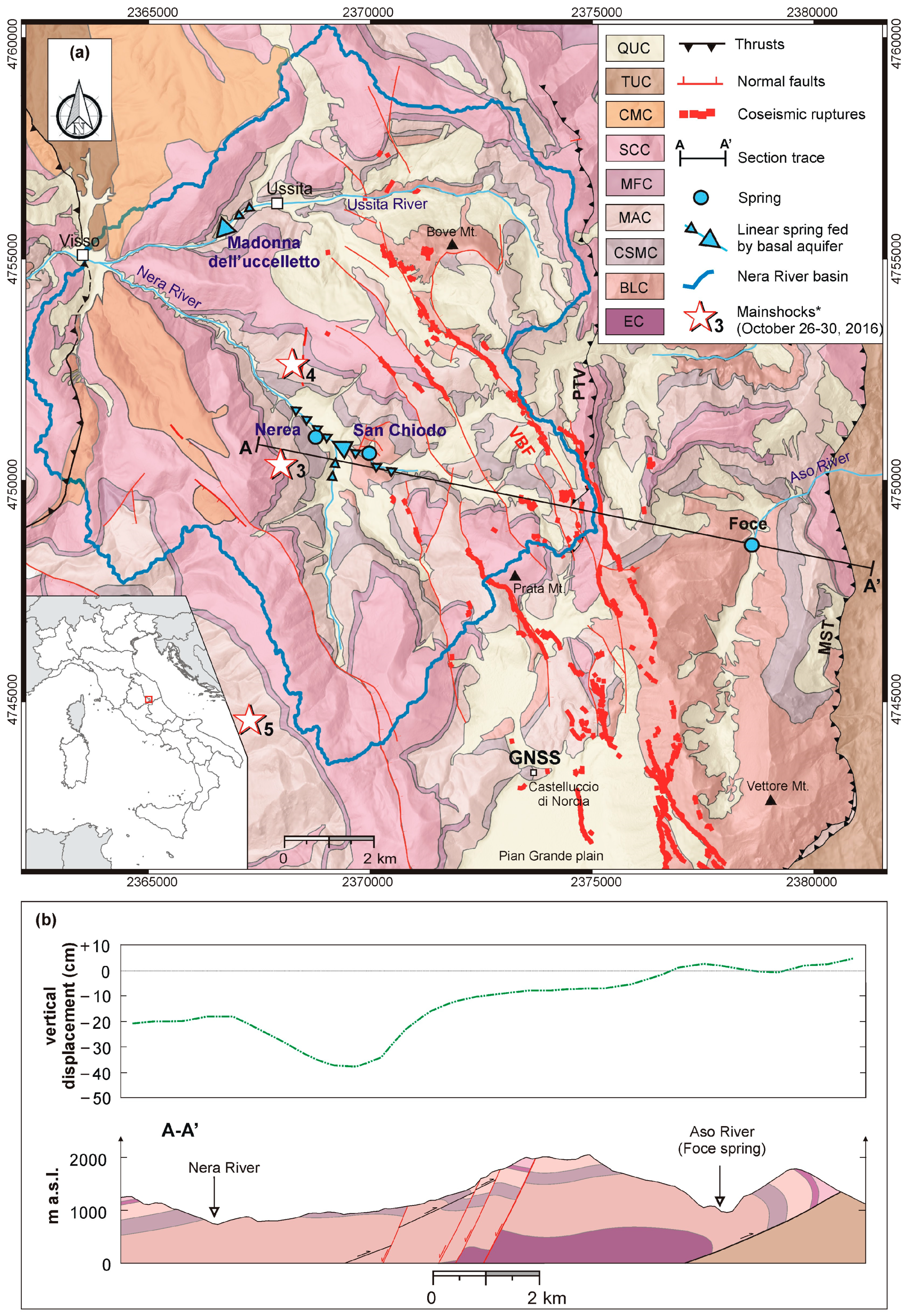
2.1. Geological Structural and Hydrogeological Setting

The area investigated in this study is located in the mountainous region of the Sibillini Mountains (northern Apennines) in Central Italy. The stratigraphic sequence of this part of the Apennine consists of Meso-Cenozoic carbonate multilayer formations (Fms) of the Umbria-Marche succession and siliciclastic foredeep deposits of the Laga Fm [32]. Figure 1a shows the hydrogeological map of the upper part of the Nera River basin. It is based on a new geological survey, which checked and updated the geological map published by [32]; rocks are described considering the stratigraphic relationships and focusing on the hydrogeological properties, e.g., grouping them in hydrogeological complexes [33,34,35,36].
The sequence starts with Upper Triassic evaporites, including anhydrides and dolomites (evaporites Fm). These rocks are not exposed in the study area and are characterized by a general low permeability (Evaporites Complex, EC). Upward, the sequence continues with shallow-water carbonates (Calcare Massiccio Fm) with a variable thickness of 600 to 700 m. In the Jurassic structural lows, a thick prevalent pelagic sequence was deposited. Micritic limestones represented the basal deposition of structural lows with nodules of chert (Corniola Fm). Being high fractured/karstified limestones, the Calcare Massiccio and Corniola host the basal aquifer with a maximum thickness of ca. 900 m (Basal Limestones Complex, BLC). The pelagic sequence continues with Calcareous Siliceous Marly Complex (CSMC, including Rosso Ammonitico, Marne del Serrone, Calcari a Posidonia, and Calcari Diasprigni Fms), characterized by low relative permeability. The subsequent deposition of Maiolica Fm occurred on both structural highs and lows, with a variable thickness from 150 to a maximum of 400 m, respectively (Maiolica Complex, MAC). Stratified and fractured limestones characterize the hydrogeological complex, with high relative permeability. Due to high permeability, it represents the middle aquifer. The sequence continues upward with the Marne a Fucoidi Fm, a marly rock with low relative permeability (Marne a Fucoidi Complex, MFC). Marly-limestones (about 400 m thick) were then deposited above the Marne a Fucoidi Fm; it includes the Scaglia Calcarea Complex (SCC, Scaglia Rossa and Scaglia Bianca), characterized by a moderate relative permeability. Above the SCC, Scaglia Variegata and Scaglia Cinerea Fms are deposited, composed of marls and marly limestones with low permeability (Calcareous Marly Complex, CMC). The subsequent Miocene marly units (Schlier and Bisciaro) and siliciclastic Laga Fm are mainly exposed in the eastern sector of the studied area. Most of these Fms are characterized by moderate or low permeability (Terrigenous Units Complex, TUC).
Formations belonging to the hydrogeological complexes were involved in distinct tectonic phases since the Jurassic. First, extensional tectonics was associated with the thinning of the Adriatic continental margin during Late Jurassic [32], involving the Basal Limestones Complex. Since the late Miocene, the whole limestone multilayer was affected by a compressional phase that produced important shortening of this part of the Apennines with a typical fold and thrust belt [37,38]. The Sibillini Mountains thrust (MST, Figure 1a) represented the main regional compressional structure [39], marking the tectonic boundary between the Mesozoic–Paleogene limestone sequence at its hanging-wall and the Late Miocene–Early Pliocene Laga sequence (Flysch della Laga Fm, [40]) at its footwall. A more internal compressional structure is represented by the Pizzo Tre Vescovi thrust (PTV, Figure 1a).
The compressional structures were subsequently crosscut by the NNW-SSE trending normal faults due to the prevalent extensional Quaternary tectonic phase [41,42]. These faults are still active and responsible for historical seismicity and represent preferential drainage paths of groundwater in the basal aquifer, which usually hinder the transversal groundwater exchanges [35,43].

2.2. Seismic Sequence and Co-Seismic Effects

The study area was struck by a long and intensive seismic sequence during 2016 and 2017 (Figure 1a), characterized by the occurrence of nine mainshocks with moment magnitude, Mw > 5.0 (Table 1). The seismic sequence was due to a system of mainly NNW-SSE striking and WSW dipping normal faults, as shown by the focal mechanism of the main shocks, the distribution of the aftershocks, and significant co-seismic ruptures [46,47,48,49,50,51,52,53].
The main seismogenic normal faults activated during the seismic sequence were the Vettore Mt.–Bove Mt. fault systems (VBF) to the north and the Laga (LAF) fault systems to the south [55]. This study is focused on the northern sector affected by the VBF segment.
In particular, the southern portion of the VBF and the northern portion of the LAF (Figure 1a) were activated during the 24 August Mw 6.0 Accumoli event, which enucleated at their overlapping area, at a depth of 8 km [51,56]. The 26 October Mw 5.9 Visso event enucleated at a depth of 4 km [57] and activated the northern part of the VBF, while during the 30 October Mw 6.5 Norcia event, the VBF was activated to the south and center. The average co-seismic throw of the entire sequence is ~0.3 m [52,53] and the activation of the VBF during the largest events produced important surface ruptures developed along major and minor fault segments as shown in Figure 1a [51,53]. Figure 1b shows a cross section roughly oriented WE with co-seismic displacements produced by the October 30, 2016, seismic sequence as taken from Valerio et al. [45]. Geodetic measurements, using the Global Navigation Satellite System (GNSS) technique together with the available surface deformation field obtained on the basis of the DInSAR technique, registered the co-seismic and immediately post-seismic deformation of the two major October shocks surrounding the VBF [44]. One of the GNSS stations (Figure 1a) recorded westward horizontal displacements of 419 mm and subsidence of 707 mm (with 95% confidence errors), with a total off-fault vertical displacement between footwall and hanging-wall blocks of 736 mm in correspondence of the northern sector of the VBF.

3. Materials and Methods

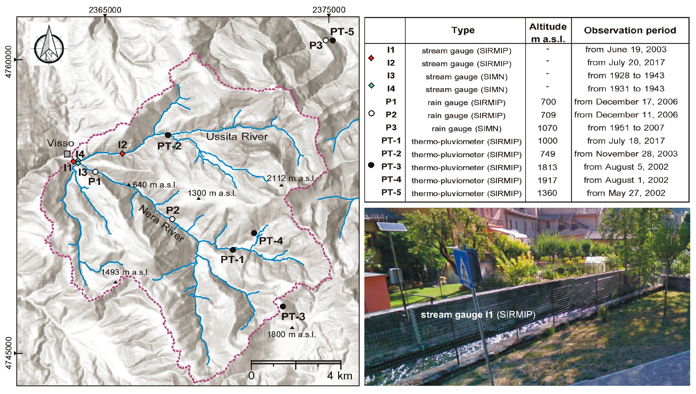
3.1. Meteorological Data and Techniques of Analysis

The study of river discharge fed by regional aquifers requires reliable meteorological data. According to Cambi et al. [13], as for other mountain regions in Central Italy, often few data are available to define the hydrogeological scheme. Figure 2 shows all the thermo-pluviometric stations located within the Nera River catchment at Visso section.
As for other locations in the Mediterranean region, the upper part of the Nera River catchment has had changes in the data acquisition network over time; the overall monitoring network has moved from the Servizio Idrografico e Mareografico Nazionale (SIMN) to the Civil Protection Agency of Marche Region (SIRMIP) during the beginning of the 2000s, resulting in lack of data often coupled with the relocation of some stations. To check the consistency of rainfall data, the double-mass analysis was used [57]. This method compares cumulated rainfall data of a single station with that of other stations in the area, allowing the individuation of abrupt deviations produced by instrument malfunctions and/or relocations. As recently reported by Caloiero et al. [19], lack of spatially distributed data can be overcome due to the increased availability of meteorological satellites. The Global Precipitation Measurement (GPM) provides monthly rainfall data on an approximately 10 × 10 km grid across the globe from April 2014 to the present. The latest release of the Integrated Multi-satellitE Retrievals for Global Precipitation Measurement product (IMERG, Version 6B-Final) fused GPM estimates with those collected by the TRMM satellite (Tropical Rainfall Measuring Mission), operating during 2000–2015 (https://gpm.nasa.gov/data/imerg, accessed on 25 May 2021). The Nera River catchment is included in a cell having the following lat-long coordinates: 42.45–13.05; and 42.55–13.15. Rainfall monthly data are downloaded from https://disc.gsfc.nasa.gov/datasets/GPM_3IMERGM_06/summary?keywords=%22IMERG%20final%22 (accessed on 25 May 2021). Due to the complex topography in mountain regions, checking the performance of satellite data is necessary to achieve analyses that are as realistic as possible [58,59,60]. To quantify the performance of GPM-IMERG data, Pearson’s Correlation Coefficient (CC, Equation (1)), Nash-Sutcliffe efficiency (NSE, Equation (2)), Root Mean Square Error (RMSE, Equation (3)), and the relative bias (rBias, Equation (4)) are used; the latter reflects the systematic bias between the satellite and the ground observations [61].
CC = i = 1 n ( G i G ¯ ) · ( S i S ¯ ) i = 1 n ( G i G ¯ ) 2 · i = 1 n ( S i S ¯ ) 2
NSE = 1 i = 1 n ( S i G i ) 2 i = 1 n ( G i G ¯ ) 2
RMSE = i = 1 n ( S i G i ) 2 n
rBias = i = 1 n ( S i G i ) 2 i = 1 n G i · 100
where:
Si = satellite precipitation estimate (mm/month)
Gi = rain gauge observation (mm/month)
S ¯ = mean satellite precipitation estimate (mm/month)
G ¯ = mean gauge precipitation observation (mm/month)
Reliable monthly rainfall datasets are useful to check the frequency and length of droughts, which affect the groundwater recharge of hydrogeological systems. Worldwide, the Standardized Precipitation Index (SPI, [62]) is used as an effective drought index for detecting and characterizing meteorological droughts. According to WMO [63], for the computation at least 20–30 years of monthly rainfall data are needed. In the SPI computation the data are fitted to a gamma probability distribution and then transformed into a normal distribution. For a given data time series Xi as X1, X2….Xn, the SPIi is defined by Equation (5).
SPI i = X i X ¯ S x
where X ¯ is the arithmetic mean of rainfall and S x is the standard deviation. According to McKee et al. [62], wet periods occur when SPI values are higher than 1 while drought periods occur when SPI is lower than −1. SPI equal to zero implies that there is no deviation from the mean. Table 2 shows the classification for the SPI values.
Monthly precipitation (P) and temperature (T) have been used to compute the monthly evapotranspiration (ETR) using the Thornthwaite and Mather [64] method. This method is still useful when no data concerning radiation, air humidity, etc.—necessary to apply more modern methods—are available, as occurred for the study area [59,65]. The computation of ETR was carried out by using the software developed by Čadro [66]. Surplus monthly data (S = P-ETR) were then computed to individuate the period with no recharge (P = ETR), i.e., the river discharge is fed only by the groundwater stored in the hydrological system, which empties as the depletion phase proceeds.

3.2. Discharge Data

Daily stream levels (H) of the Nera River were collected from the SIRMIP on-line monitoring network on the I1 river section (Figure 2), which also includes its main tributary (Ussita stream, I2 stream gauge). By using the rating curve published by SIRMIP (http://app.protezionecivile.marche.it/sol/indexjs.sol?lang=it, accessed on 25 May 2021), daily stream discharge values (Q) were computed from January of 2016. No substantial anthropic modification occurred in the catchment in the last decades that could have influenced SW–GW interactions through the river system. Apart from the construction of a fluent hydroelectric plant close to the P1 station (Figure 2), a drinking water intake was built near Castelsantangelo sul Nera village in the 1980s (San Chiodo spring, Figure 1). As the water is piped out of the Nera River catchment, the amount of drinking water withdrawn was added to the river discharge data; it corresponds to 0.150 m3/s from January of 2016 to February of 2018 and 0.200 m3/s from March of 2018 to today [67]. As reported by Di Matteo et al. [24], in addition to recent monitoring data, some historical discharges from the SIMN monitoring network (I3 and I4 in Figure 2) are also available (1928–1943 period).

3.3. Models for River Recession Curves

The study of the discharge during periods with no recharge (recession curve) provides insightful hydrologic information about the hydrogeological properties of the system feeding the river, at least in terms of average or equivalent values. Several conceptual models for recession curves have been developed to describe the discharge during the recession period. In the hydrogeological practice the exponential formula (EF) is extensively used (Equation (6), [68,69]). Although EF was developed for porous media (Darcian laminar flow), it has also been widely applied to fractured aquifers characterized by low hydraulic gradients and velocity [70,71,72]. When these conditions are not met (turbulent flow), the straight-line equation (SL) can describe the recession process in fractured and karst aquifers (Equation (7), [73,74]). The rate of change of the discharge (RCD) is computed making the first derivative of Equations (6) and (7), obtaining Equations (8) and (9) for EF and SL, respectively,
Q t =   Q o · e α E · t
Q t =   Q o α TL
RCD EF = α E · Q t  
RCD SL = α ETL  
where:
Qt and Qo = discharge at time t and at the beginning of recession period (m3/d)
αE = Maillet recession coefficient (d−1)
αTL = Torricelli-like recession coefficient (m3/d2)
RCDEF = rate of change of the discharge of EF equation (m3/d2)
RCDTL = rate of change of the discharge of SL equation (m3/d2)
According to Rorabaugh [75], and Kovacs and Perrochet [76], αE is linked to the aquifer characteristics by Equation (10).
α E = π · k · H S · L 2
where:
k = aquifer’ hydraulic conductivity (m/d)
H = aquifer thickness (m)
L = length of the one-dimensional domain (m)
S = storativity (dimensionless)

4. Results

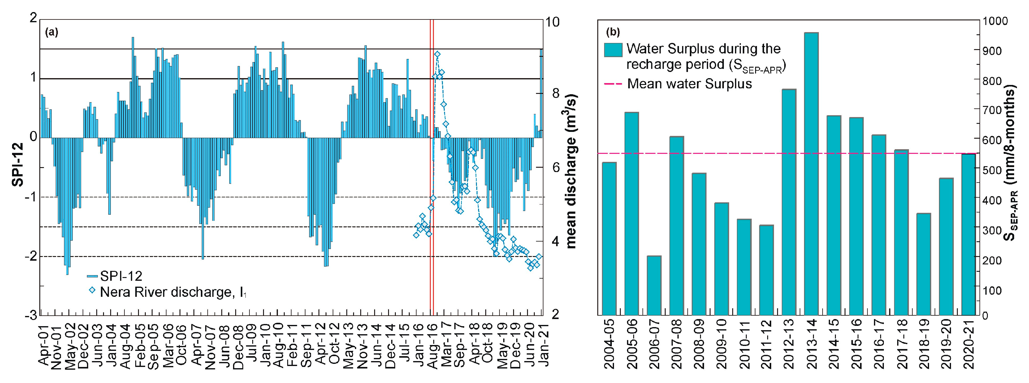
4.1. Rainfall-Water Surplus Analysis

The recharge of aquifers is affected by prolonged drought periods, the evaluation of number and frequency of which require reliable rainfall data. Figure 3 shows the results of the double mass analysis; data of Ussita station (PT-2) are compared with those of ENDESA (P1) and M. Prata (PT-3) stations. The cumulative rainfall of PT-2 and P1—located at similar altitude—is aligned along a straight line with no abrupt deviations. On the contrary, an abrupt change between the years 2008 and 2010 is observed by comparing the cumulated rainfall data of PT-2 with PT-3. The latter shows lower cumulative rainfall despite being located 1050 m higher than PT-1. The double-mass analysis results for the 2002–2020 period found the Ussita station to be the most reliable in the study area.
As illustrated in Section 2.1, the computation of SPI requires at least 20–30 years of monthly rainfall data [63]. The Ussita station does not meet this requirement, i.e., it is not suitable for SPI analysis. Among the available stations (Figure 2), only the Bolognola station could be useful for this analysis (P3 and PT-5). Unfortunately, in 2007, the historical rain gauge (P3, SIMN) was removed, and the new station was located at a higher elevation than the historical one (PT-5, SIRMIP), i.e., the rain gauge was moved from 1070 m a.s.l. to 1370 m a.s.l. Under these conditions, the aggregation of the two-time periods (1951–2007 and 2007–2020) was not successful; therefore, the data were not used for the SPI computation. In this framework, satellite data can be a valid alternative for this analysis, especially in data-scarce regions. The results of the application of some accuracy indices show that the correlation among monthly GPM-IMERG satellite data and rainfall at the Ussita gauge reaches a CC value equal to 0.76, a NSE of 0.99, a RMSE of 4.5 mm, and a rBias of about 24%, confirming that satellite data tend to slightly overestimate rainfall data as already recorded by Navarro et al. [60] along the Apennine chain of the Italian peninsula. The results of statistical evaluations indicate that—within the limits of use of satellite data in mountain areas (e.g., effects of topography, etc.)—the performance of GPM-IMERG allows the use of this dataset to compute the SPI during the 2000–2020 period. Similar results were recently obtained by Caloiero et al. [19], who used the GPM-IMERG data to calculate SPI values for the Italian peninsula. Figure 4a shows the SPI-12 computed over the last two decades; prolonged drought events are detected in 2001–2003, 2007, 2012, and 2018. Three moderate to near normal wet periods are interposed between these events. Similar findings—even if with slightly different intensities and with some difference for 2018—were obtained by Valigi et al. [25] for the Pescara di Arquata Spring recharge area, located about 20 km southeast of the upper part of the Nera River catchment.
Figure 4b shows the cumulated water surplus (S) during the recharge periods (September–April); weather data of the Ussita station are used for the computation. During the observation period, the mean S was about 550 mm/8-months with the highest values from 2013–14 to 2017–18, confirming the results of SPI analysis. On the contrary, in the 2018–19 and 2019–20 periods, S values were 100–200 mm lower than the mean, corresponding to the moderate/severe dry periods highlighted with the SPI-12 (Figure 4a).

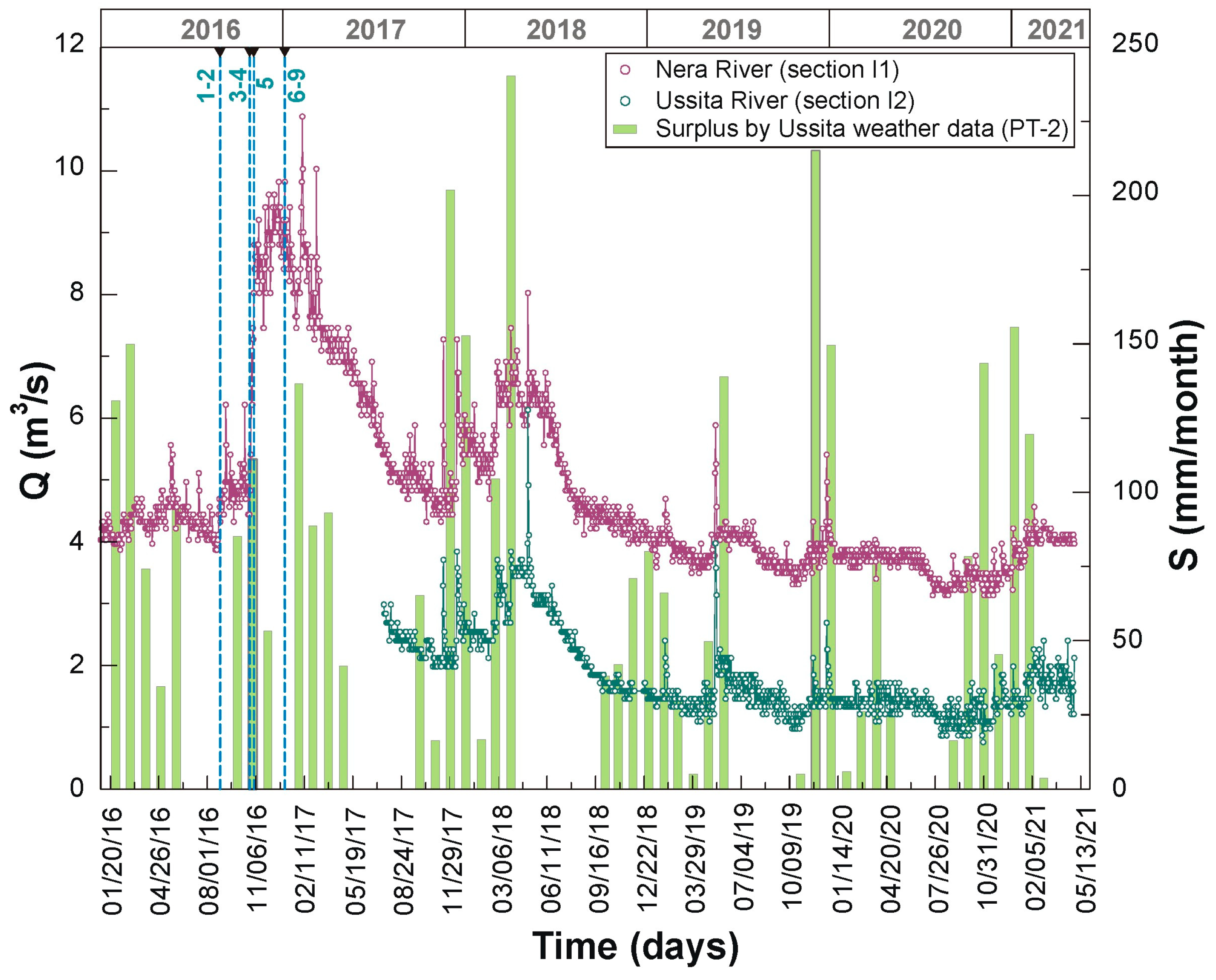
4.2. River Hydrograph Analysis

The flow regime of the Nera River was studied considering the available daily discharge data. According to the SIRMP monitoring system, reliable data were recorded during the 2016–2021 period (Figure 5). These data include both pre- and post-seismic phases.
The 30 October 2016, earthquake (n. 5 in Figure 5) produced the abrupt discharge rising observed during November–January of 2016 with an increase of about 4.8 m3/s. A small peak flow rate had already been recorded on 24 August 2016, connected with the Accumoli-Norcia earthquakes (ns. 1–2 in Figure 5). Figure 5 also shows the monthly water surplus, computed according to the Thornthwaite and Mather [64] method, and daily discharge data of the Ussita River. The discharge hydrograph of this sub-catchment overlaps the Nera River one with some differences during the late August–September periods of 2017 and 2018. In these two periods, the recession phase of the Ussita River continued while that of the Nera River stopped after receiving some recharge that did not occur in the Ussita catchment.
Considering periods with no aquifer recharge (water surplus S = 0 in Figure 5) the pre- and post-seismic recession curves were collected. After the individuation of months with S = 0, a deep analysis was carried out to separate consecutive days characterized by a decrease in discharge values, avoiding days with discharge increases in response to the previous effective rainfalls. These curves help to investigate the relationship between aquifer hydrogeological properties and groundwater discharge to the river. The results of the analysis of the 2019 and 2020 depletion phases are presented in Figure 6, moving to the discussion section for the comparison with previous studies published in the study area in the two years following the earthquake. The EF recession model describes both 2019 and 2020 recession curves as a result of the best-fit analysis, indicating that the hydrogeological system feeding the river empties with a Darcian laminar flow. The two curves show similar a recession coefficient αE, −2.1 × 10⁻³ day−1 and −2.3 × 10⁻³ day−1 for 2019 and 2020, respectively.

5. Discussion

Updates on the response of the Nera River discharge to the 2016 seismic sequence are discussed, taking into consideration the meteorological conditions during pre- and post-seismic phases. During the two years after the 2016 seismic sequence (2017 and 2018), the peak of river discharge after the autumn–spring recharge period was very high compared with 2019 and 2020 (Figure 5). The high discharge value recorded in January of 2017 was mainly linked to co-seismic effects (e.g., increased aquifer permeability and pore water pressure). Moreover, as reported by Petitta et al. [22], the impressive increase in spring and river discharge observed in the upper Nera River may be correlated with the subsidence induced by the toe of VBF—as already recorded by GNSS station (Figure 1a)—which might have created an additional “squeezing effect” in the core of the Sibillini Mountains aquifer. Barberio et al. [77] reported some changes in hydrochemical characteristics of water of the basal aquifer feeding the San Chiodo spring (Figure 1a), such as an increase in the content of three metals (Cr, Fe, and V) and one metalloid (As) four months before or roughly in conjunction with the 2016 seismic sequence, respectively. Rosen et al. [78] reported no change in most of the major ions and in δ18OH2O and δ2HH2O of waters of the Nerea spring (Figure 1a), the recharge area of which is characterized by the basal aquifer extending towards SE including the Vettore Mountain faulting systems deeply affected by co-seismic ruptures (Figure 1). In detail, concentrations of SO4 showed no change after the 30 October 2016, earthquake and trace element concentrations returned to pre-earthquake concentrations by the end of November, 2016. The authors concluded that the hydrochemical dynamics suggested within-aquifer changes instead of mixing with another aquifer, geothermal fluids, or aquifer breaching. Recently, Fronzi et al. [79] presented updated hydrogeochemical results for the Castelsantangelo sul Nera area—also fed by basal aquifer and located slightly upstream to the Nerea spring—showing some sampling points with an increase in SO4 content and some others with no increase after the mainshock. The different results reported by [78,79] highlight the complexity of processes that occurs in a hydrogeological system highly influenced by normal faults and co-seismic fracturing systems. In other words, sampling points collected along the normal faults interacting with Triassic evaporites aquiclude below the Mt. Vettore–Pian Grande Plain show increases in SO4, which is not evident in other zones—also fed by basal aquifer—where normal faults and co-seismic fracturing did not play a significant role.
Mastrorillo et al. [23], by a mechanism named “Aquifer Fault Rupture”, hypothesized a shift eastward of the piezometric divide, severely penalizing the aquifers in the eastern side of the Sibillini Mountains. The authors left open whether or not the modified piezometric divide would recover to its original position. Our results on the Upper Nera River catchment (western part of the Apennine chain) show that co-seismic effects on GW lasted up to at least 2018 by analyzing river discharges at the Visso gauge. The peak discharge that occurred in 2018 is preceded by a recharge period characterized by a water surplus in line with or slightly above the historical mean. The maximum discharge was 1.3 times higher than that recorded in 2016 (pre-seismic conditions); the latter was preceded by about four years of very high water surplus values, which did not produce the high spring flows recorded in 2018 (Figure 4b). After about five years from the seismic sequence, the comparison of pre- and post-seismic recession curves can contribute to understanding what processes are taking place and whether or not permanent changes have taken place. Table 3 shows the recession processes and recession coefficients computed on the available recession periods. Figure 7 shows all the available pre- and post-seismic recession curves, sorted from the highest discharge to the lowest.
Curves with similar recession processes and recession coefficients have been merged using the strip method [80,81,82]. This approach allows obtaining a Master Recession Curve (MRC); the Root Mean Square Error (RMSE) criterion has been used to choose the best time-shifting to join the curves. A recent study carried out by Di Matteo et al. [24] highlighted that the SL equation described the recession curves of the two years following the seismic sequence (2017 and 2018). A permeability enhancement of the aquifer feeding the Nera River—due to cleaning of fractures and the co-seismic fracturing in the recharge area—coupled with an increase in groundwater flow velocity can explain this process, which lasted up to 2018. Fronzi et al. [26] also recorded consistent variations in the hydraulic conductivity distribution throughout carbonate aquifers related to the VBF system activation. Figure 7 also includes the most recent recession curves (2019 and 2020), which fit very well with the pre-seismic ones (Equation (11)), represented by the EF equation (Darcian flow).
Q t =   Q o · e α E · t = 491,264.40 · e 0.0025 · t       ( R 2 = 0.98 )
Considering that the recession process recovered to the same pre-earthquake conditions—at least for two consecutive years (2019 and 2020)—and αE values are similar to the pre-seismic ones (Table 1), it can be deduced that hydrogeological changes induced by the seismic sequence seem to be almost recovered. As Equation (10) shows, co-seismic effects could have changed other parameters than aquifer hydraulic conductivity. It is interesting to point out that if the length of the one-dimensional domain (L) had increased (i.e., the recharge area had enlarged due to aquifer breaching), we should have expected much lower αE than pre-earthquake conditions. The permeability recovery after high magnitude earthquakes has been documented in a wide range of hydrogeological settings; most documented recovery times are about two years as obtained for the Nera River [27,28,83]. As Manga et al. [84] discussed, the mechanism of recovery is not clear because of the complexity and inaccessibility of the subsurface; a combination of mechanical and geochemical processes can cause the return of the enhanced permeability to approximately the pre-seismic value. Aben et al. [85] reported a list of possible recovery mechanisms of earthquake-related fracture damage including time-dependent mechanical recovery of micro and macro-cracks, sealing by mineral precipitation (e.g., calcite), resulting in fracture sealing, and fracture closure by pressure solution creep, the latter two act on longer time scales than mechanical ones. Based on the discharge at Visso gauge (I1), regardless of the mechanism that led to the recovery of the hydrogeological properties of the aquifer feeding the Nera River, it is important to emphasize again that, the emptying process seems to be restored to the same as it was before the 2016 earthquake. Since the reservoir in 2019 and 2020 empties at rates lower than 2017 and 2018, the hydrogeological system—as it was in the past—is less vulnerable to prolonged droughts such as those that are increasingly affecting the Apennine area of Central Italy.

6. Conclusions

The 2016 seismic sequence deeply affected the hydrogeological system of the upper part of the Nera River catchment—the waters of which are of strategic importance to the territory’s economy. Through analysis of the geological-structural and hydrogeological data about five years after the seismic sequence, the following conclusions can be drawn:
The peak river flow recorded in 2017 and 2018 did not occur in 2019 and 2020—the latter was preceded by a drought period well detected by the SPI, which affected the recharge of groundwater, and consequently the river discharge;
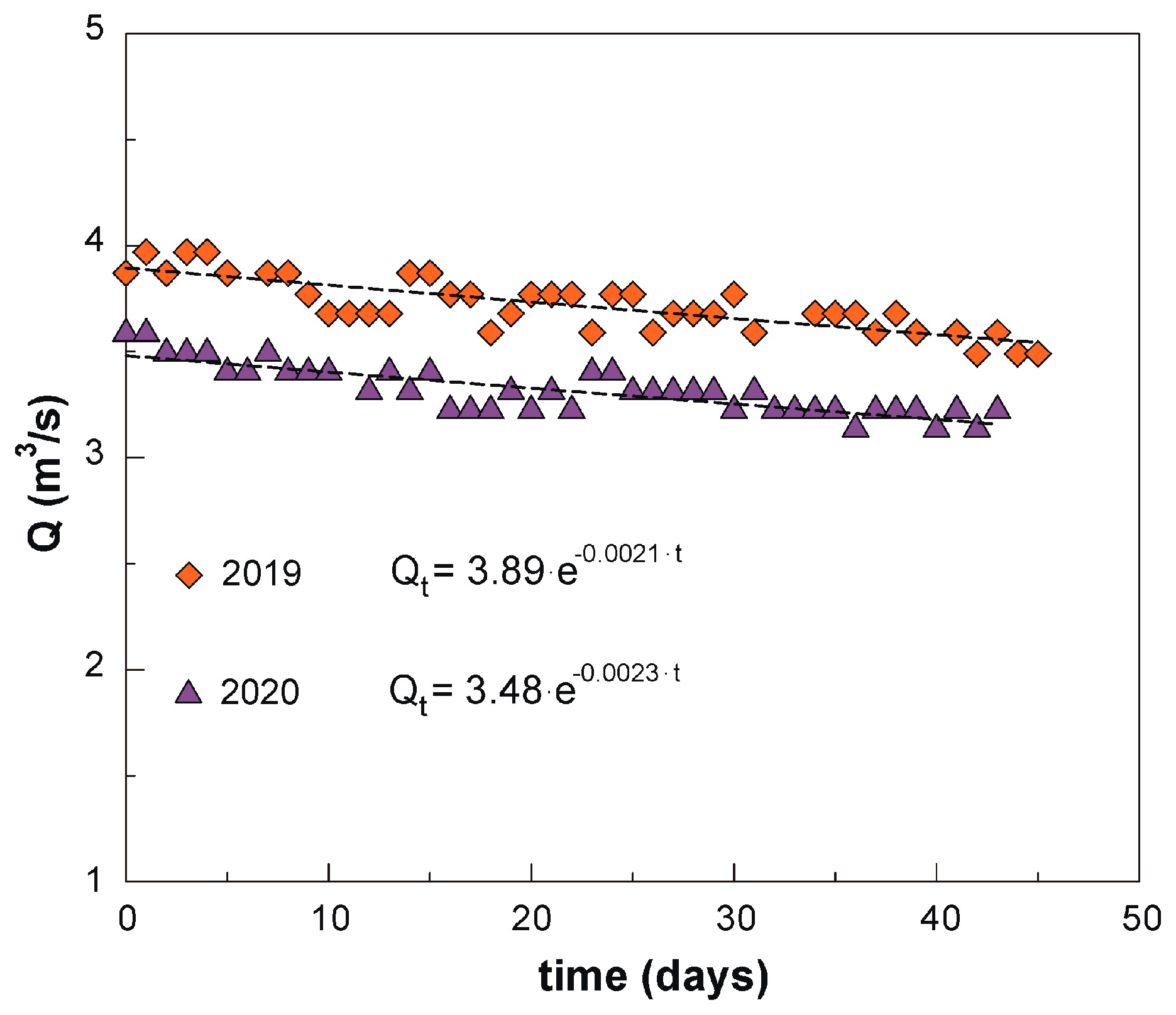
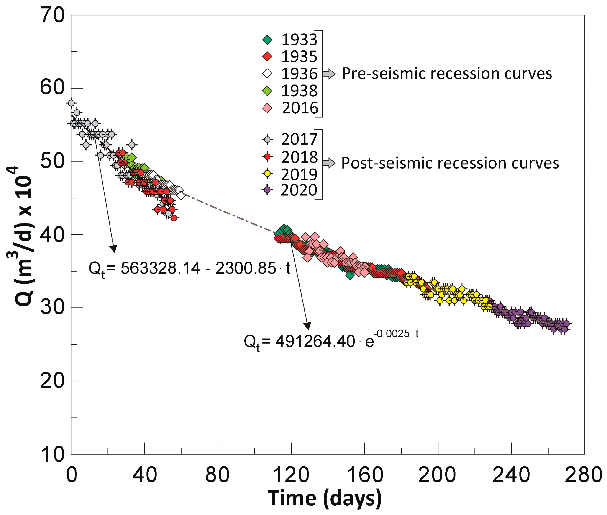
The rapid depletion observed during the 2017 and 2018 recession periods (straight line equation and turbulent flow) were not detected in 2019 and 2020, where both recession process and recession coefficients seem to be restored to the same as prior to the 2016 earthquake (exponential equation and Darcian flow);
Co-seismic effects on the hydrogeological system (e.g., increased aquifer permeability and pore water pressure) appear to have recovered after two years from the 2016 seismic sequence, as documented in other systems around the world affected by strong earthquakes.
Based on the discharge data representing the whole hydrogeological system feeding the Nera River, the findings reported here contribute to understanding processes and dynamics of fractured carbonate aquifers located in geologically and climatically complex regions, which are useful for water management. The results need to be further refined by continuing the monitoring and also with consideration of the response of hydrogeological systems located east of the Apennine chain.

Supplementary Materials

The following are available online at https://0-www-mdpi-com.brum.beds.ac.uk/article/10.3390/hydrology8030097/s1, Table S1: discharge data for the selected pre-and post-recession periods.

Author Contributions

Conceptualization, L.D.M. and C.P.; methodology, L.D.M., A.C., M.P. and C.P.; validation, L.D.M., A.C., M.P. and C.P.; formal analysis, L.D.M. and A.C.; investigation, L.D.M., A.C., M.P. and C.P.; data curation, L.D.M., A.C., M.P. and C.P.; writing—original draft preparation, L.D.M., A.C., M.P. and C.P.; writing—review and editing, L.D.M., A.C., M.P. and C.P.; visualization, L.D.M., A.C., M.P. and C.P.; supervision, L.D.M.; project administration, L.D.M. All authors have read and agreed to the published version of the manuscript.

Funding

This research received no external funding.

Institutional Review Board Statement

Not applicable.

Informed Consent Statement

Not applicable.

Data Availability Statement

Data are contained in the supplementary material.

Acknowledgments

The authors wish to thank the Marche Region—Civil Protection Service for discharge data.

Conflicts of Interest

The authors declare no conflict of interest.

References

  1. Winter, T.C.; Harvey, J.W.; Franke, O.L.; Alley, W.M. Ground Water and Surface Water: A Single Resource; US Geological Survey: Denver, CO, USA, 1999; Volume 1139, pp. 1–88. Available online: https://pubs.usgs.gov/circ/circ1139 (accessed on 15 May 2021).
  2. Sophocleous, M. Interactions between groundwater and surface water: The state of the science. Hydrogeol. J. 2002, 10, 52–67. [Google Scholar] [CrossRef]
  3. Jolly, I.D.; McEwan, K.L.; Holland, K.L. A review of groundwater–surface water interactions in arid/semi-arid wetlands and the consequences of salinity for wetland ecology. Ecohydrology 2008, 1, 43–58. [Google Scholar] [CrossRef]
  4. Fleckenstein, J.H.; Krause, S.; Hannah, D.M.; Boano, F. Groundwater-surface water interactions: New methods and models to improve understanding of processes and dynamics. Adv. Water Res. 2010, 33, 1291–1295. [Google Scholar] [CrossRef]
  5. Li, M.; Liang, X.; Xiao, C.; Cao, Y. Quantitative Evaluation of Groundwater–Surface Water Interactions: Application of Cumulative Exchange Fluxes Method. Water 2020, 12, 259. [Google Scholar] [CrossRef] [Green Version]
  6. Guzman, P.; Batelaan, O.; Wyseure, G. Comparative analysis of base flow recession curves for different Andean catchments. Geophys. Res. Abs. 2012, 14, 8318. Available online: https://meetingorganizer.copernicus.org/EGU2012/EGU2012-8318.pdf (accessed on 18 May 2021).
  7. Berghuijs, W.; Woods, R.; Hrachowitz, M. A precipitation shift from snow towards rain leads to a decrease in streamflow. Nat. Clim. Chang. 2014, 4, 583–586. [Google Scholar] [CrossRef] [Green Version]
  8. Boni, C.; Bono, P.; Capelli, G. Schema idrogeologico dell’Italia Centrale. Mem. Soc. Geol. It. 1986, 35, 991–1012. (In Italian). Available online: https://www.idrogeologiaquantitativa.it/wordpress/wp-content/uploads/2009/11/Pubb_1986_Schema_Italia_Centrale.pdf (accessed on 18 May 2021).
  9. Cencetti, C.; Dragoni, W.; Nejad Massoum, M. Contributo alle conoscenze delle caratteristiche idrogeologiche del Fiume Nera (Appennino centro-settentrionale). Geol. Appl. Idrogeol. 1989, 24, 191–210. [Google Scholar]
  10. Preziosi, E.; Romano, E. From a hydrostructural analysis to the mathematical modelling of regional aquifers (Central Italy). It. J. Eng. Geol. Environ. 2009, 1, 183–198. [Google Scholar] [CrossRef]
  11. Boni, C.; Baldoni, T.; Banzato, F.; Cascone, D.; Petitta, M. Hydrogeological study for identification, characterization and management of groundwater resources in the Sibillini Mountains National Park (Central Italy). It. J. Eng. Geol. Environ. 2010, 2, 21–39. [Google Scholar] [CrossRef]
  12. Altava-Ortiz, V.; Llasat, M.C.; Ferrari, E.; Atencia, A.; Sirangelo, B. Monthly rainfall changes in Central and Western Mediterranean basins, at the end of the 20th and beginning of the 21st centuries. Int. J. Climatol. 2011, 31, 1943–1958. [Google Scholar] [CrossRef]
  13. Cambi, C.; Valigi, D.; Di Matteo, L. Hydrogeological study of data-scarce limestone massifs: The case of Gualdo Tadino and Monte Cucco structures (Central Apennines, Italy). Bollet. Geofisica Teorica Appl. 2010, 51, 345–360. [Google Scholar]
  14. Longobardi, A.; Villani, P. Trend analysis of annual and seasonal rainfall time series in the Mediterranean area. Int. J. Climatol. 2010, 30, 1538–1546. [Google Scholar] [CrossRef]
  15. Di Matteo, L.; Valigi, D.; Cambi, C. Climatic characterization and response of water resources to climate change in limestone areas: Some considerations on the importance of geological setting. J. Hydrol. Eng. 2013, 18, 773–779. [Google Scholar] [CrossRef] [Green Version]
  16. Diodato, N.; Büntgen, U.; Bellocchi, G. Mediterranean winter snowfall variability over the past millennium. Int. J. Climatol. 2019, 39, 384–394. [Google Scholar] [CrossRef] [Green Version]
  17. Gentilucci, M.; Barbieri, M.; Lee, H.S.; Zardi, D. Analysis of rainfall trends and extreme precipitation in the Middle Adriatic Side, Marche Region (Central Italy). Water 2019, 11, 1948. [Google Scholar] [CrossRef] [Green Version]
  18. Caporali, E.; Lompi, M.; Pacetti, T.; Chiarello, V.; Fatichi, S. A review of studies on observed precipitation trends in Italy. Int. J. Climatol. 2021, 41, E1–E25. [Google Scholar] [CrossRef]
  19. Caloiero, T.; Caroletti, G.N.; Coscarelli, R. IMERG-Based Meteorological Drought Analysis over Italy. Climate 2021, 9, 65. [Google Scholar] [CrossRef]
  20. Valigi, D.; Luque Espinar, J.A.; Di Matteo, L.; Cambi, C.; Pardo Iguzquiza, E.; Rossi, M. Analysis of drought conditions and their effects on Lake Trasimeno (Central Italy) levels. It. J. Groundwater 2016, 17–215, 39–47. [Google Scholar] [CrossRef]
  21. Diodato, N.; Bellocchi, G. Climate control on snowfall days in peninsular Italy. Theor. Appl. Climatol. 2020, 140, 951–961. [Google Scholar] [CrossRef]
  22. Petitta, M.; Mastrorillo, L.; Preziosi, E.; Banzato, F.; Barberio, M.D.; Billi, A.; Cambi, C.; De Luca, G.; Di Carlo, G.; Di Curzio, D.; et al. Water table and discharge changes associated with the 2016–2017 seismic sequence in central Italy: Hydrogeological data and a conceptual model for fractured carbonate aquifers. Hydrogeol. J. 2018, 26, 1009–1026. [Google Scholar] [CrossRef] [Green Version]
  23. Mastrorillo, L.; Saroli, M.; Viaroli, S.; Banzato, F.; Valigi, D.; Petitta, M. Sustained post-seismic effects on groundwater flow in fractured carbonate aquifers in Central Italy. Hydrol. Proc. 2020, 34, 1167–1181. [Google Scholar] [CrossRef] [Green Version]
  24. Di Matteo, L.; Dragoni, W.; Azzaro, S.; Pauselli, C.; Porreca, M.; Bellina, G.; Cardaci, W. Effects of earthquakes on the discharge of groundwater systems: The case of the 2016 seismic sequence in the Central Apennines, Italy. J. Hydrol. 2020, 583, 124509. [Google Scholar] [CrossRef]
  25. Valigi, D.; Fronzi, D.; Cambi, C.; Beddini, G.; Cardellini, C.; Checcucci, R.; Mastrorillo, L.; Mirabella, F.; Tazioli, A. Earthquake-induced spring discharge modifications: The Pescara di Arquata spring reaction to the august–october 2016 Central Italy earthquakes. Water 2020, 12, 767. [Google Scholar] [CrossRef] [Green Version]
  26. Fronzi, D.; Di Curzio, D.; Rusi, S.; Valigi, D.; Tazioli, A. Comparison between Periodic Tracer Tests and Time-Series Analysis to Assess Mid-and Long-Term Recharge Model Changes Due to Multiple Strong Seismic Events in Carbonate Aquifers. Water 2020, 12, 3073. [Google Scholar] [CrossRef]
  27. Manga, M.; Rowland, J.C. Response of Alum Rock springs to the October 30, 2007 earthquake and implications for the origin of increased discharge after earthquakes. Geofluids 2009, 9, 237–250. [Google Scholar] [CrossRef]
  28. Geballe, Z.M.; Wang, C.-Y.; Manga, M. A permeability-change model for water level changes triggered by teleseismic waves. Geofluids 2011, 11, 302–308. [Google Scholar] [CrossRef]
  29. Rojstaczer, S.; Wolf, S.; Michel, R. Permeability enhancement in the shallow crust as a cause of earthquake induced hydrological changes. Nature 1995, 373, 237–239. [Google Scholar] [CrossRef]
  30. Wang, C.Y.; Manga, M. New streams and springs after the 2014 Mw 6.0 South Napa earthquake. Nat. Commun. 2015, 6, 7597. [Google Scholar] [CrossRef] [PubMed] [Green Version]
  31. Binda, G.; Pozzi, A.; Michetti, A.M.; Noble, P.J.; Rosen, M.R. Towards the understanding of hydrogeochemical seismic responses in karst aquifers: A retrospective meta-analysis focused on the Apennines (Italy). Minerals 2020, 10, 1058. [Google Scholar] [CrossRef]
  32. Pierantoni, P.; Deiana, G.; Galdenzi, S. Stratigraphic and structural features of the Sibillini mountains (Umbria-Marche Apennines, Italy). It. J. Geosci. 2013, 132, 497–520. [Google Scholar] [CrossRef]
  33. Boscherini, A.; Checcucci, R.; Natale, G.; Natali, N. Carta Idrogeologica della Regione Umbria (scala 1:100.000). Giornale Geol. Appl. 2005, 2, 399–404. [Google Scholar] [CrossRef]
  34. Civita, M. Idrogeologia Applicata e Ambientale; Casa editrice ambrosiana: Milano, Italy, 2005; p. 800. (In Italian) [Google Scholar]
  35. Viaroli, S.; Mirabella, F.; Mastrorillo, L.; Angelini, S.; Valigi, D. Fractured carbonate aquifers of Sibillini Mts. (Central Italy). J. Maps 2021, 17, 140–149. [Google Scholar] [CrossRef]
  36. Valigi, D.; Cambi, C.; Checcucci, R.; Di Matteo, L. Transmissivity Estimates by Specific Capacity Data of Some Fractured Italian Carbonate Aquifers. Water 2021, 13, 1374. [Google Scholar] [CrossRef]
  37. Mazzoli, S.; Pierantoni, P.P.; Borraccini, F.; Paltrinieri, W.; Deiana, G. Geometry, segmentation pattern and displacement variations along a major Apennine thrust zone, central Italy. J. Struct. Geol. 2005, 27, 1940–1953. [Google Scholar] [CrossRef]
  38. Porreca, M.; Minelli, G.; Ercoli, M.; Brobia, A.; Mancinelli, P.; Cruciani, F.; Giorgetti, C.; Carboni, F.; Mirabella, F.; Cavinato, G.; et al. Seismic reflection profiles and subsurface geology of the area interested by the 2016–2017 earthquake sequence (Central Italy). Tectonics 2018, 37, 1116–1137. [Google Scholar] [CrossRef]
  39. Koopman, A. Detachment Tectonics in the Central Apennines, Italy. Ph.D. Thesis, Instituut voor Aardwetenschappen RUU, 1983. Available online: http://dspace.library.uu.nl/bitstream/handle/1874/216947/Koopman-Anton-30-1983.pdf?sequence=1&isAllowed=y (accessed on 31 May 2021).
  40. Centamore, E.; Adamoli, L.; Berti, D.; Bigi, G.; Bigi, S.; Casnedi, R.; Cantalamessa, G.; Fumanti, F.; Morelli, C.; Micarelli, A.; et al. Carta geologica dei bacini della Laga e del Cellino e dei rilievi carbonatici circostanti (Marche meridionali, Lazio nordorientale, Abruzzo settentrionale). Stud. Geol. Camert. 1992, 2, Tavola 1. Available online: http://193.204.8.201:8080/jspui/bitstream/1336/782/1/Vol.%2091-2%20Cap.%2018%20Allegato%202.pdf (accessed on 31 May 2021).
  41. Lavecchia, G.; Brozzetti, F.; Barchi, M.; Menichetti, M.; Keller, J.V. Seismotectonic zoning in east-central Italy deduced from an analysis of the Neogene to present deformations and related stress fields. GSA Bullet. 1994, 106, 1107–1120. [Google Scholar] [CrossRef]
  42. Porreca, M.; Fabbrizzi, A.; Azzaro, S.; Pucci, S.; Del Rio, L.; Pierantoni, P.P.; Giorgetti, C.; Roberts, G.P.; Barchi, M.R. 3D geological reconstruction of the M. Vettore seismogenic fault system (Central Apennines, Italy): Cross-cutting relationship with the M. Sibillini thrust. J. Struct. Geol. 2020, 131, 103938. [Google Scholar] [CrossRef]
  43. Tarragoni, C. Determinazione della “quota isotopica” del bacino di alimentazione delle principali sorgenti dell’alta Valnerina. Geol. Romana 2006, 39, 55–62. [Google Scholar]
  44. De Guidi, G.; Vecchio, A.; Brighenti, F.; Caputo, R.; Carnemolla, F.; Di Pietro, A.; Lupo, M.; Maggini, M.; Marchese, S.; Messina, D.; et al. Brief communication: Co-seismic displacement on 26 and 30 October 2016 (Mw = 5.9 and 6.5)–earthquakes in central Italy from the analysis of a local GNSS network. Nat. Hazards Earth Syst. Sci. 2017, 17, 1885–1892. [Google Scholar] [CrossRef] [Green Version]
  45. Valerio, E.; Tizzani, P.; Carminati, E.; Doglioni, C.; Pepe, S.; Petricca, P.; De Luca, C.; Bignami, C.; Solaro, G.; Castaldo, R.; et al. Ground Deformation and Source Geometry of the 30 October 2016 Mw 6.5 Norcia Earthquake (Central Italy) Investigated Through Seismological Data, DInSAR Measurements, and Numerical Modelling. Remote Sens. 2018, 10, 1901. [Google Scholar] [CrossRef] [Green Version]
  46. EMERGEO Working Group. Coseismic effects of the 2016 Amatrice seismic sequence: First geological results. Ann. Geophys. 2016, 59, Fast Track 5. [Google Scholar] [CrossRef]
  47. Aringoli, D.; Farabollini, P.; Giacopetti, M.; Materazzi, M.; Paggi, S.; Pambianchi, G.; Pierantoni, P.P.; Pistolesi, E.; Pitts, A.; Tondi, E. The August 24th 2016 Accumoli earthquake: Surface faulting and Deep-Seated Gravitational Slope Deformation (DSGSD) in the Monte Vettore area. Ann. Geophys. 2016, 59, Fast Track 5. [Google Scholar] [CrossRef]
  48. Lavecchia, G.; Castaldo, R.; de Nardis, R.; De Novellis, V.; Ferrarini, F.; Pepe, S.; Brozzetti, F.; Solaro, G.; Cirillo, D.; Bonano, M.; et al. Ground deformation and source geometry of the 24 August 2016 Amatrice earthquake (Central Italy) investigated through analytical and numerical modeling of DInSAR measurements and structural-geological data. Geophys. Res. Lett. 2016, 43, 389–398. [Google Scholar] [CrossRef]
  49. Livio, F.; Michetti, A.M.; Vittori, E.; Gregory, L.; Wedmore, L.; Piccardi, L.; Tondi, E.; Roberts, G.; and Central Italy Earthquake Working Grooup. Surface faulting during the August 24, 2016, Central Italy earthquake (Mw 6.0): Preliminary results. Ann. Geophys. 2016, 59, Fast Track 5. [Google Scholar] [CrossRef]
  50. Galli, P.; Galadini, F.; Pantosti, D. Twenty years of paleoseismology in Italy. Earth Sci. Rev. 2008, 88, 89–117. [Google Scholar] [CrossRef]
  51. Pucci, S.; De Martini, P.M.; Civico, R.; Villani, F.; Nappi, R.; Ricci, T.; Azzaro, R.; Brunori, C.A.; Caciagli, M.; Cinti, F.R.; et al. Coseismic ruptures of the24 August 2016, Mw 6.0 Amatrice earthquake (central Italy). Geophys. Res. Lett. 2017, 44. [Google Scholar] [CrossRef]
  52. Civico, R.; Pucci, S.; Villani, F.; Pizzimenti, L.; De Martini, P.M.; Nappi, R.; Wedmore, L. Surface ruptures following the 30 October 2016 Mw 6.5 Norcia earthquake, central Italy. J. Maps 2018, 14, 151–160. [Google Scholar] [CrossRef] [Green Version]
  53. Villani, F.; Pucci, S.; Civico, R.; De Martini, P.M.; Cinti, F.R.; Pantosti, D. Surface faulting of the 30 October 2016 Mw 6.5 central Italy earthquake: Detailed analysis of a complex coseismic rupture. Tectonics 2018, 37, 3378–3410. [Google Scholar] [CrossRef]
  54. Michele, M.; Chiaraluce, L.; Di Stefano, R.; Waldhauser, F. Fine-Scale Structure of the 2016–2017 Central Italy Seismic Sequence From Data Recorded at the Italian National Network. J. Geophys. Res. Solid Earth 2020, 125, e2019JB018440. [Google Scholar] [CrossRef]
  55. Barchi, M.R.; Carboni, F.; Michele, M.; Ercoli, M.; Giorgetti, C.; Porreca, M.; Azzaro, S.; Chiaraluce, L. The influence of subsurface geology on the distribution of earthquakes during the 2016-–2017 Central Italy seismic sequence. Tectonophysics 2021, 807, 228797. [Google Scholar] [CrossRef]
  56. Chiaraluce, L.; Di Stefano, R.; Tinti, E.; Scognamiglio, L.; Michele, M.; Casarotti, E.; Cattaneo, M.; De Gori, P.; Chiarabba, C.; Monachesi, G.; et al. The 2016 central Italy seismic sequence: A first look at the mainshocks, aftershocks, and source models. Seismol. Res. Lett. 2017, 88, 757–771. [Google Scholar] [CrossRef]
  57. Searcy, J.K.; Hardison, C.H. Double-Mass Curves; US Government Printing Office: Washington, DC, USA, 1960; Volume 1541, p. 66.
  58. Vernimmen, R.R.E.; Hooijer, A.; Aldrian, E.; Van Dijk, A.I.J.M. Evaluation and bias correction of satellite rainfall data for drought monitoring in Indonesia. Hydrol. Earth Syst. Sci. 2012, 16, 133–146. [Google Scholar] [CrossRef] [Green Version]
  59. Di Matteo, L.; Dragoni, W.; Maccari, D.; Piacentini, S.M. Climate change, water supply and environmental problems of headwaters: The paradigmatic case of the Tiber, Savio and Marecchia rivers (Central Italy). Sci. Total Environ. 2017, 598, 733–748. [Google Scholar] [CrossRef] [PubMed]
  60. Navarro, A.; García-Ortega, E.; Merino, A.; Sánchez, J.L.; Kummerow, C.; Tapiador, F.J. Assessment of IMERG precipitation estimates over Europe. Remote Sens. 2019, 11, 2470. [Google Scholar] [CrossRef] [Green Version]
  61. Saouabe, T.; El Khalki, E.M.; Saidi, M.E.M.; Najmi, A.; Hadri, A.; Rachidi, S.; Jadoud, M.; Tramblay, Y. Evaluation of the GPM-IMERG precipitation product for flood modeling in a semi-arid mountainous basin in Morocco. Water 2020, 12, 2516. [Google Scholar] [CrossRef]
  62. McKee, T.B.; Doesken, N.J.; Kleist, J. The relationship of drought frequency and duration to time scales. In Proceedings of the 8th Conference on Applied Climatology, Anaheim, CA, USA, 17–22 January 1993; Volume 17, pp. 179–183. [Google Scholar]
  63. WMO-World Meteorological Organization. Standardized precipitation index user guide. M.; Svoboda, M. Hayes and D. Wood. (WMO-No. 1090), Geneva. Available online: www.wamis.org/agm/pubs/SPI/WMO_1090_EN.pdf (accessed on 25 May 2021).
  64. Thornthwaite, C.W.; Mather, J.R. The water balance. Centerton: Drexel institute of technology, laboratory of climatology. Publ. Climatol. 1955, 8, 104. [Google Scholar]
  65. Shuttleworth, W.J. Putting the “vap” into evaporation. Hydrol. Earth Syst. Sci. 2007, 11, 210–244. [Google Scholar] [CrossRef] [Green Version]
  66. Čadro, S. Excel sheet for Potential Evapotranspiration (PET) and Soil Water Balance Calculation Based on Thornthwaite Method (1948). Available online: https://www.researchgate.net/profile/Sabrija_Cadro/publication/309740661_Thornthwaite_Potential_Evapotranspiration_PET_and_Water_Balance_1948/data/582187e808aeccc08af8d4eb/Thornthwaite-Evapotranspiration-PET-and-Water-Balance-1948.xlsx (accessed on 25 May 2021).
  67. D.R. 35/2018. Fiume Nera–Derivazione Dalle Opere di Captazione Presso la Sorgente San Chiodo. AATO 3 Marche Centro–Società Acquedotto del Nera (MC). Marche Region Law with Subsequent Modifications and Additions. Available online: http://www.ato3marche.it/assemblea-di-ambito/atti-e-documenti-assemblea-di-ambito/decreti-del-presidente/2018-2/1455-decreto-del-presidente-n-12-2018-del-08-06-2018/file (accessed on 25 May 2021).
  68. Boussinesq, J. Essai sur la théorie des eaux courantes du movement non permanent des eaux souterraines. Acad. Sci. Inst. Fr. 1877, 23, 252–260. [Google Scholar]
  69. Maillet, E. Essais D’hydraulique Souterraine et Fluviale; Librairie Sci.: Paris, France, 1905; p. 218. [Google Scholar]
  70. Scanlon, B.R.; Mace, R.E.; Barrett, M.E.; Smith, B. Can we simulate regional groundwater flow in a karst system using equivalent media models? Case study Barton springs Edwards Aquifer, USA. J. Hydrol. 2003, 276, 137–158. [Google Scholar] [CrossRef]
  71. Rehrl, C.; Birk, S. Hydrogeological characterisation and modelling of spring catchments in a changing environment. Aust. J. Earth Sci. 2010, 103, 106–117. [Google Scholar] [CrossRef] [Green Version]
  72. Dragoni, W.; Mottola, A.; Cambi, C. Modeling the effects of pumping wells in spring management: The case of Scirca spring (Central Apennines, Italy). J. Hydrol. 2013, 493, 115–123. [Google Scholar] [CrossRef]
  73. Coutagne, A. Les variations de dèbit en pèriode non influencèe par les prècipitations. In Le dèbit d’Inflitration (Corrèlations Fluviales Internes)–2me Partie, Meteorologie et Hydrologie; La Houille Blanche: Grenoble, France, 1948; pp. 416–436. [Google Scholar]
  74. Bonacci, O. Karst Hydrology With Special Reference to the Dinaric Karst; Springer: Heidelberg, Germany, 1987; p. 184. [Google Scholar]
  75. Rorabough, M.I. Estimating changes in bank storage and grounwater contribution to streamflow. Int. Assoc. Sci. Hydro. Publ. 1964, 63, 432–441. [Google Scholar]
  76. Kovács, A.; Perrochet, P.A. quantitative approach to spring hydrograph decomposition. J. Hydrol. 2008, 352, 16–29. [Google Scholar] [CrossRef]
  77. Barberio, M.D.; Barbieri, M.; Billi, A.; Doglioni, C.; Petitta, M. Hydrogeochemical changes before and during the 2016 Amatrice-Norcia seismic sequence (central Italy). Sci. Rep. 2017, 7, 11735. [Google Scholar] [CrossRef]
  78. Rosen, M.R.; Binda, G.; Archer, C.; Pozzi, A.; Michetti, A.M.; Noble, P.J. Mechanisms of earthquake-induced chemical and fluid transport to carbonate groundwater springs after earthquakes. Water Res. Res. 2018, 54, 5225–5244. [Google Scholar] [CrossRef]
  79. Fronzi, D.; Mirabella, F.; Cardellini, C.; Caliro, S.; Palpacelli, S.; Cambi, C.; Valigi, D.; Tazioli, A. The Role of Faults in Groundwater Circulation before and after Seismic Events: Insights from Tracers, Water Isotopes and Geochemistry. Water 2021, 13, 1499. [Google Scholar] [CrossRef]
  80. Singh, V.P. Hydrologic Systems: Watershed Modeling; Prentice-Hall: Denver, CO, USA, 1989; p. 448. [Google Scholar]
  81. Tallaksen, L.M. A review of baseflow recession analysis. J. Hydrol. 1995, 165, 349–370. [Google Scholar] [CrossRef]
  82. Posavec, K.; Parlov, J.; Nakić, Z. Fully automated objective-based method for master recession curve separation. Groundwater 2010, 48, 598–603. [Google Scholar] [CrossRef]
  83. Elkhoury, J.E.; Brodsky, E.E.; Agnew, D.C. Seismic waves increase permeability. Nature 2006, 441, 1135–1138. [Google Scholar] [CrossRef] [PubMed]
  84. Manga, M.; Beresnev, I.; Brodsky, E.E.; Elkhoury, J.E.; Elsworth, D.; Ingebritsen, S.E.; Mays, D.C.; Wang, C.Y. Changes in permeability caused by transient stresses: Field observations, experiments, and mechanisms. Rev. Geophys. 2012, 50, 1–24. [Google Scholar] [CrossRef]
  85. Aben, F.M.; Doan, M.L.; Gratier, J.P.; Renard, F. Experimental postseismic recovery of fractured rocks assisted by calcite sealing. Geophys. Res. Lett. 2017, 44, 7228–7238. [Google Scholar] [CrossRef] [Green Version]
Figure 1. (a) Hydrogeological map of the upper part of the Nera River catchment with the mainshocks of 26–30 October 2016, seismic sequence (information on earthquakes are in Table 1). EC—Evaporitic-dolomitic Complex; BLC—Basal Limestones complex; CSMC—Calcareous Siliceous Marly Complex; MAC—Maiolica Complex; MFC—Marne a Fucoidi Complex; SCC—Scaglia Calcarea Complex; CMC—Calcareous Marly Complex; TUC—Terrigenous units complex; QUC—Quaternary Units Complex; VBFMt. Vettore-Mt. Bove fault systems; PTV—Pizzo Tre Vescovi thrust; SMTSibillini Mts. Thrust; GNSSGlobal Navigation Satellite System station [44]. (b) Cross section roughly oriented WE (co-seismic displacements produced by the 30 October 2016 seismic sequence are taken from [45]).
Hydrology 08 00097 g001
Figure 2. Nera River catchment at Visso section (A = 130 km2) with the location and description of the hydro-meteorological stations.
Hydrology 08 00097 g002
Figure 3. Double-mass curves for detecting the consistency of rainfall data. (a) Comparison between PT-2 and P1. (b) Comparison between PT-2 and PT-3. The location of rainfall stations is in Figure 2.
Hydrology 08 00097 g003
Figure 4. (a) A period of 12-months of SPI computed by using GMP-IMERG rainfall data with mean monthly discharge of the Nera River at section I1 (Figure 2). The two vertical red bars indicate the August 24 and the 30 October 2016, seismic shocks. (b) Cumulated water surplus (S)—based on the Thornthwaite and Mather [64] methodduring the recharge period (8 months from September to April).
Hydrology 08 00097 g004
Figure 5. Hydrograph of the Nera River and Ussita River with monthly surplus calculated by using meteorological data of the Ussita station. The blue numbers adjacent to the dashed lines indicate the main earthquakes with moment magnitude (Mw) higher than 5.0 that occurred during the 2016–2017 seismic sequences in Central Italy (information about the earthquakes are reported in Table 1).
Hydrology 08 00097 g005
Figure 6. Recession curves for 2019 and 2020. Discharge data of the Nera River are recorded at section I1 (Figure 2).
Hydrology 08 00097 g006
Figure 7. Pre- and post-seismic recession curves for the Nera River at section I1. Discharge data are in the supplementary materials (Table S1).
Hydrology 08 00097 g007
Table 1. Mainshocks of the 2016–2017 seismic sequence (modified from [54]).
LocalizationDataMwHypocentral Depth (km)
1Accumoli (42.70–13.70)24 August 20166.04.65
2Norcia (42.79–13.15)24 August 20165.44.87
3Castel Santangelo sul Nera (42.88–13.12)26 October 20165.43.46
4Visso (42.91–13.09)26 October 20165.92.47
5Norcia (42.83–13.11)30 October 20166.55.78
6Capitignano (42.56–13.29)18 January 20175.17.87
7Capitignano (42.55–13.28)18 January 20175.57.72
8Capitignano (42.52–13.29)18 January 20175.48.38
9Barete (42.48–13.28)18 January 20175.09.43
Table 2. Classification scale for the SPI values [63].
ClassConditionSPI Values
1Extremely wetSPI > 2
2Very wet 1.5 ≤ SPI < 2
3Moderately wet 1.0 ≤ SPI < 1.5
4Near normal −1.0 ≤ SPI < 1.0
5Moderately dry −1.5 ≤ SPI < −1.0
6Severely dry −2.0 ≤ SPI < −1.5
7Extremely drySPI ≤ −2.0
Table 3. Recession models that best describe the Nera River discharges (Section I1 in Figure 2) during the available recession periods.
YearRecession PeriodRecession ModelRecession Coefficient
19337 July–15 SeptemberEF−2.5 × 10⁻³ d−1
19354 June–23 AugustEF−2.2 × 10⁻³ d−1
19361 June–21 JuneEF−2.9 × 10⁻³ d−1
193822 June–12 JulyEF−3.2 × 10⁻³ d−1
201619 July–18 AugustEF−2.8 × 10⁻³ d−1
201713 June–6 AugustSL−2274 m3/d2
201827 June–27 JulySL−2267 m3/d2
201916 August–29 SeptemberEF−2.1 × 10⁻³ d−1
202010 July–14 AugustEF−2.3 × 10⁻³ d−1
Publisher’s Note: MDPI stays neutral with regard to jurisdictional claims in published maps and institutional affiliations.

