Acoustic Streaming and Its Applications

Abstract

Broadly speaking, acoustic streaming is generated by a nonlinear acoustic wave with a finite amplitude propagating in a viscid fluid. The fluid volume elements of molecules, $dV$, are forced to oscillate at the same frequency as the incident acoustic wave. Due to the nature of the nonlinearity of the acoustic wave, the second-order effect of the wave propagation produces a time-independent flow velocity (DC flow) in addition to a regular oscillatory motion (AC motion). Consequently, the fluid moves in a certain direction, which depends on the geometry of the system and its boundary conditions, as well as the parameters of the incident acoustic wave. The small scale acoustic streaming in a fluid is called “microstreaming”. When it is associated with acoustic cavitation, which refers to activities of microbubbles in a general sense, it is often called “cavitation microstreaming”. For biomedical applications, microstreaming usually takes place in a boundary layer at proximity of a solid boundary, which could be the membrane of a cell or walls of a container. To satisfy the non-slip boundary condition, the flow motion at a solid boundary should be zero. The magnitude of the DC acoustic streaming velocity, as well as the oscillatory flow velocity near the boundary, drop drastically; consequently, the acoustic streaming velocity generates a DC velocity gradient and the oscillatory flow velocity gradient produces an AC velocity gradient; they both will produce shear stress. The former is a DC shear stress and the latter is AC shear stress. It was observed the DC shear stress plays the dominant role, which may enhance the permeability of molecules passing through the cell membrane. This phenomenon is called “sonoporation”. Sonoporation has shown a great potential for the targeted delivery of DNA, drugs, and macromolecules into a cell. Acoustic streaming has also been used in fluid mixing, boundary cooling, and many other applications. The goal of this work is to give a brief review of the basic mathematical theory for acoustic microstreaming related to the aforementioned applications. The emphasis will be on its applications in biotechnology.

1. Introduction

When a continuous sinusoidal acoustic wave propagates in an inviscid fluid, it forces the fluid elements to oscillate sinusoidally in the wave propagation direction; if the corresponding particle velocity $\mathit{v}$ of a fluid element is much smaller than the speed of sound, $c_0$, in the fluid, this acoustic wave is called a “linear acoustic wave”. Its main characteristic is that the superposition principal holds during its propagation, and $c_0$ is not a function of the frequency of the acoustic wave. Consequently, the wave shape will not change during propagation, and the time-averaged flow velocity of a fluid element is zero. However, when the amplitude of the acoustic wave increases, the above-described condition for the superposition principal is no longer valid; this type of acoustic wave is called a “finite amplitude nonlinear acoustic wave”. Therefore, the time-average of the second order of each fluid element’s oscillatory velocity has a time-independent (DC) component velocity in addition to a sinusoidal oscillatory velocity; this DC velocity is called “acoustic streaming”. It is important to be aware that acoustic streaming only occurs in a viscous fluid. General speaking, acoustic streaming can be divided into two categories according to the scale of the fluid system (l) in relation to the wavelength (λ) of the acoustic wave. When l >> λ, it is called “Eckart” streaming [1]. Eckart streaming is generated by the energy transfer from the acoustic wave to the kinetic energy of the DC flow motion through the dissipation of the acoustic wave in a bulk fluid via the absorption of the fluid. While $\delta \ll l\ll \lambda$, it belongs to “Rayleigh” streaming, where $\delta =\sqrt{\frac{\mu }{\pi \rho f}}$ is called the viscous boundary layer thickness, $\mu$ is dynamic viscosity, $\rho$ is the density of the fluid, and $f$ is frequency of the acoustic wave. Rayleigh streaming is also called “boundary related” streaming [2,3,4]. The goal of this article is to give readers a brief review of the basic theoretical background related to acoustic streaming, i.e., how it is generated by an acoustic wave. The main focus is on the acoustic streaming in a fluid generated by applications of ultrasound of sub-megahertz and megahertz frequency. Its major applications include promoting fluid mixing and targeted drug delivery in the biomedical field.

The Reynolds number (Re) is a parameter used to describe the characteristics of the flow, which is defined as Re = ρvl/$\mu$. Due to the small scale of dimension l of a microfluidic device, the associated Reynolds number is also small, and as a result, turbulence usually cannot form, although it may involve with a vortex-like rotational flow to a certain degree, which will be discussed in detail in a later section. In summary, acoustic streaming induced by ultrasound provides a simple and effective way to induce fluid mixing. Biomedical applications involve the application of the shear stress associated with microstreaming generated by oscillating microbubbles in microfluidic devices for in vitro targeted drug delivery biological assays [5,6] via a technique called “sonoporation”. Like electroporation [7], sonoporation refers to ultrasound-triggered partial cell membrane disruption to form pores on the membrane with dimensions from tens of nanometers to several micrometers, significantly enhancing cell membrane permeability to macromolecules. If the pores are minute, they may be repaired by the living cell automatically; therefore, it is called “reparable sonoporation”. Thus, sonoporation is a potential tool for gene- and drug-delivery applications in medicine. The widely accepted biophysical mechanism of sonoporation involves the shear stress due to the rapid drop of microstreaming velocity near a boundary [8].

The acoustic pressure wave causes microscopic gas pockets stably residing on the wall of a microfluidic device or cell membranes to oscillate and grow via a process of asymmetric rectified diffusion, i.e., the gas in-flow during the bubble expansion due to the rarefaction half cycles of the incident wave is greater than the gas out flow when the bubble is compressed by the other half of the compression periods of the incident acoustic wave on site [9]; consequently, the gas pocket grows to become a so-called “cavitation bubble” of sub-millimeter to millimeter scale, which happens to be the resonance size corresponding to incident acoustic frequency of sub-megahertz and megahertz. The high amplitude oscillations of the nonlinear cavitation bubble excited by the incident acoustic wave generates microstreaming in the proximity of bubbles. Steady DC flow patterns were observed near an oscillating bubble [10,11]. In the vicinity of an oscillating bubble, the microstreaming DC velocity and the oscillatory AC velocity drop rapidly near the membrane of the cell in the proximity of the cavitation bubble to satisfy the nonslip boundary condition at the membrane. The velocity gradient generates the local DC and AC shear stress to the membrane. It was observed that the DC shear stress plays the dominant role [12]. This maximum DC shear stress is given by the following equation: $S_{\max }=2{\pi }^{\frac{3}{2}}{\mathit{v}}_0^2{(\frac{\rho \mu }{f})}^{\frac{1}{2}}/{\mathit{R}}_0$, where ${\mathit{v}}_0$ is the amplitude of the sinusoidal particle velocity and ${\mathit{R}}_0$ is the radius of the equilibrium bubble or other vibrating source [12,13]. The cell assembles are “massaged” by the shear stress. Depending on the strength and duration of the “massage”, the porosity on the cell membrane may be generated and the cell membrane becomes temporarily permeable to DNA and drug molecules. The intensity of the gas bubble’s oscillation can be controlled by adjusting the amplitude of the incident ultrasound. Under ultrasound of moderate intensity, the porous cell membrane can be patched by the cell itself. Reparable sonoporation can be used as a technique for targeted drug delivery [14,15,16,17,18,19,20,21,22]. Acoustic streaming DC flow generated by ultrasound has also been used to deliver antibiotic chemicals to mitigate a biofilm [23,24].

Ultrasound has been widely used for clinical imaging. The encapsulated microbubbles (EMB) are used as the contrast agent, which can enhance the contrast of the ultrasound image significantly. EMB has also been used in preclinical medical applications to treat various diseases, and it plays primary role in sonoporation to deliver drugs.

Recently, the high frequency surface acoustic wave (SAW) has been applied in microfluidic systems and has received increasing attention from the research community [25]. The primary advantage of a microfluidic device is its miniaturization, whereby acoustic energy is localized to the interface of a substrate [26,27]. As a versatile method for particle manipulation, SAW-based microfluidic devices have been widely applied to manipulate various objects, such as polystyrene micro-spheres, microbubbles [28,29,30,31,32], as well as the local heating [33].

2. The Fundamental Theory of the Acoustic Streaming

The basic equations include the conservation of mass and Navier-Stokes equation of the fluid mechanics; respectively, they are:

$$\frac{\partial \rho }{\partial t}+\nabla ·\left(\rho \mathit{v}\right)=0$$

(1)

$$\rho \left(\frac{\partial \mathit{v}}{\partial t}+\mathit{v}·\nabla \mathit{v}\right)=-\nabla P+\mu {\nabla }^2\mathit{v}+(\eta +\frac{1}{3}\mu )\nabla \left(\nabla ·\mathit{v}\right)$$

(2)

where $\mathit{v}\mathrm{is}\mathrm{the}\mathrm{flow}\mathrm{velocity}\mathrm{vector},P\mathrm{is}\mathrm{the}\mathrm{pressure}\mathrm{of}\mathrm{a}\mathrm{fluid},\eta$ and $\mu$ are the bulk and the shear viscosities of the fluid respectively; both are independent of density $\rho$. Here, we assume the wave propagation is isentropic/adiabatic process. Using the Taylor expansion of the instantaneous pressure of the fluid as a function of $\rho$, $P\left(\rho \right),$ we have the following by neglecting the time dependent terms:

$$P\left(\rho \right)=P_0+c_0^2{\rho }^{\prime }+c_0{(\frac{\partial c}{\partial \rho })}_s{{\rho }^{\prime }}^2+\dots$$

(3)

where $P_0$ is the atmospheric equilibrium pressure, ${\rho }^{\prime }$ is the density fluctuation caused by the acoustic wave, $c_0$ and c are the acoustic propagation velocity for the linear and nonlinear waves of the liquid respectively, and $s$ is the entropy of the fluid. We start with

$$\mathit{v}=\epsilon {\mathit{v}}_1+{\epsilon }^2{\mathit{v}}_2+\dots ;{\rho }^{\prime }=\rho -{\rho }_0=\epsilon {\rho }_1+{\epsilon }^2{\rho }_2+\dots$$

(4)

where $\epsilon$ is a small parameter of the first-order, ${\mathit{v}}_1,{\mathit{v}}_2,{\rho }_1,{\rho }_2\mathrm{are}$ the first-order and the second-order of the particle velocities and density fluctuations respectively, we substitute Equations (3) and (4) into Equations (1) and (2), we obtain the first-order equations:

$$\frac{\partial {\rho }_1}{\partial t}+{\rho }_0\nabla ·{\mathit{v}}_1=0$$

(5)

$${\rho }_0\frac{\partial {\mathit{v}}_1}{\partial t}=-c_0^2\nabla {\rho }_1+\left(\eta +\frac{4}{3}\mu \right)\nabla \left(\nabla ·{\mathit{v}}_1\right)-\mu \nabla \times \nabla \times {\mathit{v}}_1$$

(6)

and the second-order equation:

$$\frac{\partial {\rho }_2}{\partial t}+{\rho }_0\nabla ·{\mathit{v}}_2+\nabla ·\left({\rho }_1{\mathit{v}}_1\right)=0$$

(7)

$$\begin{array}{cc}\hfill {\rho }_0\frac{\partial {\mathit{v}}_2}{\partial t}+{\rho }_1\frac{\partial {\mathit{v}}_1}{\partial t}& +{\rho }_0\left({\mathit{v}}_1·\nabla \right){\mathit{v}}_1\hfill \\ & =-c_0^2\nabla {\rho }_2-c_0{(\frac{\partial c}{\partial \rho })}_s\nabla {\rho }_1^2+\left(\eta +\frac{4}{3}\mu \right)\nabla \left(\nabla ·{\mathit{v}}_2\right)-\mu \nabla \times \nabla \times {\mathit{v}}_2\hfill \end{array}$$

(8)

The first-order acoustic field is curl-free, i.e., $\nabla \times {\mathit{v}}_1=0$. It is noted that $\left({\mathit{v}}_1·\nabla \right){\mathit{v}}_1=\nabla \left({\mathit{v}}_1^2/2\right)-{\mathit{v}}_1\times \left(\nabla \times {\mathit{v}}_1\right)=\nabla \left({\mathit{v}}_1^2/2\right)$. By using Equations (5) and (6), Equations (7) and (8) can be simplified as

$$\frac{\partial ({\rho }_2-\frac{\omega }{c_0^2})}{\partial t}+{\rho }_0\nabla ·{\mathit{v}}_2=\frac{1}{{\rho }_0{c}_0^2}\left(\eta +\frac{4}{3}\mu \right){\mathit{v}}_1·\nabla \left(\frac{\partial {\rho }_1}{\partial t}\right)$$

(9)

$$\begin{array}{cc}\hfill {\rho }_0\frac{\partial {\mathit{v}}_2}{\partial t}+c_0^2\nabla ({\rho }_2& -\frac{\omega }{c_0^2})\hfill \\ & =-c_0{(\frac{\partial c}{\partial \rho })}_s\nabla {\rho }_1^2-\frac{1}{{\rho }_0}\left(\eta +\frac{4}{3}\mu \right){\rho }_1\nabla \left(\nabla ·{\mathit{v}}_1\right)+\left(\eta +\frac{4}{3}\mu \right)\nabla \left(\nabla ·{\mathit{v}}_2\right)\hfill \\ & -\mu \nabla \times \nabla \times {\mathit{v}}_2-\nabla \left({\rho }_0{\mathit{v}}_1^2\right)\hfill \end{array}$$

(10)

where $\omega =\frac{c_0^2{\rho }_1^2}{2{\rho }_0}+\frac{{\rho }_0}{2}{\mathit{v}}_1^2$, which is the energy per unit volume of the linearized acoustic wave. Since any vector field can be expressed as the sum of its divergence and rotation, performing “$\nabla ·\text{”}$ and $\text{“}\nabla \times \text{”}$ to both sides of Equation (10), we obtain:

$$\begin{gathered} \frac{{\partial }^2{D}_2}{\partial t^2}-c_0^2\nabla ·\left(\nabla D_2\right)-\frac{1}{{\rho }_0}\left(\eta +\frac{4}{3}\mu \right){\nabla }^2(\partial D_2/\partial t)=-\frac{1}{{\rho }_0^2}\left(\eta +\frac{4}{3}\mu \right){\nabla }^2[{\mathit{v}}_1·\nabla \left(\frac{\partial {\rho }_1}{\partial t}\right)]- \\ \frac{1}{{\rho }_0^2}\left(\eta +\frac{4}{3}\mu \right)\nabla ·\frac{\partial \left({\rho }_1\nabla D_2\right)}{\partial t}-\frac{1}{{\rho }_0}\frac{\partial }{\partial t}{\nabla }^2[c_0(\frac{\partial c}{\partial \rho }{)}_s{\rho }_1^2+{\rho }_0{\mathit{v}}_1^2] \end{gathered}$$

(11)

and

$$\frac{\partial {\mathit{R}}_2}{\partial t}-\frac{\mu }{{\rho }_0}{\nabla }^2{\mathit{R}}_2=\frac{1}{{\rho }_0^3}\left(\eta +\frac{4}{3}\mu \right)(\nabla {\rho }_1\times \nabla \frac{\partial {\rho }_1}{\partial t})$$

(12)

where $D_2=\nabla ·\mathit{v}$ and ${\mathit{R}}_2=\nabla \times {\mathit{v}}_2$. Please note we have used the identity $\nabla \times \nabla \times {\mathit{R}}_2=\nabla \left(\nabla ·{\mathit{R}}_2\right)-{\nabla }^2{\mathit{R}}_2=-{\nabla }^2{\mathit{R}}_2.\mathrm{From}$ Equation (12), for an inviscid fluid, if ${\mathit{R}}_2=0\mathrm{initially}$, $\mathrm{since}\frac{\partial {\mathit{R}}_2}{\partial t}=0,$ it will keep zero for the rest of time. In other words, the vorticity ${\mathit{R}}_2$ originates from viscosity.

As an example, let us start a first-order acoustic wave as

$${\rho }_1\left(\mathit{r},f\right)=\frac{1}{c_0^2}[P_1\left(\mathit{r}\right)\cos \left(2\pi ft\right)+\nabla P_2\left(\mathit{r}\right)\sin \left(2\pi ft\right)]$$

(13)

where $P_1\left(\mathit{r}\right)\mathrm{and}{P}_2\left(\mathit{r}\right)$ are spatial functions. Thus, we obtain:

$$\nabla {\rho }_1=\frac{1}{c_0^2}[\nabla P_1\left(\mathit{r}\right)\cos \left(2\pi ft\right)+P_2\left(\mathit{r}\right)\sin \left(2\pi ft\right)]$$

(14)

$$\nabla \frac{\partial {\rho }_1}{\partial t}=\frac{2\pi f}{c_0^2}\left[-\nabla P_1\left(\mathit{r}\right)\sin \left(2\pi ft\right)+\nabla P_2\left(\mathit{r}\right)\cos \left(2\pi ft\right)\right]$$

(15)

Further from Equations (14) and (15), we obtain:

$$\nabla {\rho }_1\times \nabla \frac{\partial {\rho }_1}{\partial t}=\frac{2\pi f}{c_0^4}\nabla P_1\left(\mathit{r}\right)\times \nabla P_2\left(\mathit{r}\right)$$

(16)

here $\nabla {\rho }_1\times \nabla \frac{\partial {\rho }_1}{\partial t}$ becomes time-independent. Therefore, substituting Equation (15) into the right side of Equation (12), which becomes the steady-state given by:

$${\nabla }^2{\mathit{R}}_2=-\frac{2\pi f}{{\rho }_0^2{c}_0^4}\left(\frac{\eta }{\mu }+\frac{4}{3}\right)\nabla P_1\left(\mathit{r}\right)\times \nabla P_2\left(\mathit{r}\right)$$

(17)

In an infinite free space, the above equation has the following solution [33]:

$${\mathit{R}}_2=\nabla \times {\mathit{v}}_2=-\frac{f}{2{\rho }_0^2{c}_0^4}\left(\frac{\eta }{\mu }+\frac{4}{3}\right){\displaystyle \int }\frac{1}{\left|r-r^{\prime }\right|}\nabla P_1\left(\mathit{r}\right)\times \nabla P_2\left(\mathit{r}\right)d^3{\mathit{r}}^{\prime }$$

(18)

which implies there is a time-independent direct flow (DC flow) in a viscous fluid, which is called “acoustic streaming”. As a typical example of Eckhart’s streaming, let us consider the streaming in a finite rigid cylindrical tube of radius $\rho =a.$ We further assume the tube is terminated with a perfect absorber to avoid reflection at the end of the tube. An acoustic wave transmitter located at the mouth of the tube emanates an acoustic wave propagating along the axial direction of the tube (z-direction). The tube is completely sealed, and no energy exchange takes place with outside of it. We may let the first-order traveling wave expressed as

$$p_1\left(r,f\right)=c_0^2{\rho }_1=P\left(\rho \right)\sin \left(k_{0}z-2\pi ft\right)$$

(19)

where $P\left(\rho \right)$ is a spatial function. Noting the relationships between the polar and Cartesian coordinates: $e_{\rho }=\cos \phi e_x+\sin \phi e_y$, and $e_{\phi }=-\sin \phi e_x+\cos \phi e_y$, Equation (16) can be expressed as

$$\nabla {\rho }_1\times \nabla \frac{\partial {\rho }_1}{\partial t}=\frac{2\pi f}{c_0^4}\nabla P_1\left(\mathit{r}\right)\times \nabla P_2\left(\mathit{r}\right)=-\frac{2\pi f}{c_0^4}{k}_{0}P\left(\rho \right)e_z\times e_{\rho }=-\frac{k_0^2}{2c_0^3}\frac{d{P}^2\left(\rho \right)}{d\rho }{e}_{\phi }$$

(20)

Substituting Equations (19) and (20) into Equation (16), we obtain:

$${\nabla }^2{\mathit{R}}_2=b\frac{d{P}^2\left(\rho \right)}{d\rho }{e}_{\phi .};\mathrm{where}b=\frac{k_0^2}{2{\rho }_0^2{c}_0^3}\left(\frac{4}{3}+\frac{\eta }{\mu }\right)$$

(21)

Here ${\nabla }^2{\mathit{R}}_2$ has only $e_{\phi }$ component and independent of $\phi$. Clearly ${\mathit{R}}_2$ also has only a component in $e_{\phi }$ direction, i.e., ${\mathit{R}}_2=f\left(\rho \right)e_{\phi }$, where $f\left(\rho \right)$ satisfies

$$\left[\frac{1}{\rho }\frac{d}{d\rho }\left(\rho \frac{d}{d\rho }\right)-\frac{1}{{\rho }^2}\right]f\left(\rho \right)=b\frac{d{P}^2\left(\rho \right)}{d\rho }$$

(22)

which can be simplified as:

$$\frac{d}{d\rho }[\frac{1}{\rho }\frac{d\left(\rho f\left(\rho \right)\right)}{d\rho }]=b\frac{d{P}^2\left(\rho \right)}{d\rho }$$

(23)

Performing integration on the above equation, we obtain:

$${\mathit{R}}_2=f\left(\rho \right)e_{\phi }=[\frac{b}{\rho }{{\displaystyle \int }}_0^{\rho }{\rho }^{\prime }{P}^2\left({\rho }^{\prime }\right)d{\rho }^{\prime }+2N\rho +\frac{M}{\rho }]e_{\phi }$$

(24)

where N and M are integration constants. In order to make $f\left(\rho \right)$ is finite at $\rho =0$, M should be zero. Equation (24) becomes

$${\mathit{R}}_2=f\left(\rho \right)e_{\phi }=[\frac{b}{\rho }{{\displaystyle \int }}_0^{\rho }{\rho }^{\prime }{P}^2\left({\rho }^{\prime }\right)d{\rho }^{\prime }+2N\rho ]e_{\phi }$$

(25)

In cylindrical coordinates, we have

$$\nabla \times {\mathit{v}}_2=\frac{1}{\rho }\{\left[\frac{\partial {\mathit{v}}_{2z}}{\partial \phi }-\frac{\partial {\mathit{v}}_{2\phi }}{\partial z}\right]e_{\rho }+\left[\frac{\partial {\mathit{v}}_{2\rho }}{\partial z}-\frac{\partial {\mathit{v}}_{2z}}{\partial \rho }\right]\rho e_{\phi }+\left[\frac{\partial {\mathit{v}}_{2\phi }}{\partial \rho }-\frac{\partial {\mathit{v}}_{2\rho }}{\partial \phi }\right]e_z\}$$

(26)

As derived above, $\nabla \times {\mathit{v}}_2$ in in $e_{\phi }$ direction, ${\mathit{v}}_{2\rho }={\mathit{v}}_{2\phi }=0$, only in $z-\mathrm{direction}$ is not zero. Therefore,

$$-\frac{\partial {\mathit{v}}_{2z}}{\partial \rho }\left(\rho e_{\phi }\right)=b\underset{0}{\overset{\rho }{{\displaystyle \int }}}{\rho }^{\prime }{P}^2\left({\rho }^{\prime }\right)d{\rho }^{\prime }+2N\rho$$

(27)

we obtain

$${\mathit{v}}_{2z}\left(\rho \right)=bw\left(\rho \right)+2N\left(a^2-{\rho }^2\right)$$

(28)

where

$$w\left(\rho \right)={{\displaystyle \int }}_{\rho }^a\frac{1}{{\rho }^{″}}[{{\displaystyle \int }}_0^{{\rho }^{″}}{\rho }^{\prime }{P}^2\left({\rho }^{\prime }\right)d{\rho }^{\prime }]d{\rho }^{″}$$

(29)

Here, we used nonslip boundary condition, i.e., ${\mathit{v}}_{2z}\left(a\right)=0$. To determine the other constant N, we need another condition of flow. One reasonable condition is for a steady flow, the total mass flow at any cross section should be zero:

$${{\displaystyle \int }}_0^a{\mathit{v}}_{2z}\left(\rho \right)\rho d\rho =0$$

(30)

Equations (28)–(30) are the basic equations to determine the acoustic streaming inside a tube. As an example, we describe the pressure amplitude of an acoustic wave generated by the acoustic transducer as follows:

$$P\left(\rho \right)=P_0 as 0<\rho <{\rho }_0; P\left(\rho \right)=0, as {\rho }_0<\rho <a$$

where ${\rho }_0$ is the beam-width of the acoustic wave. We first calculate

$${{\displaystyle \int }}_0^{{\rho }^{″}}{\rho }^{\prime P^2}\left({\rho }^{\prime }\right)d{\rho }^{\prime }=\frac{1}{2}{P}_0^2{\rho }^{″2},if{\rho }^{″}<{\rho }_0; {{\displaystyle \int }}_0^{{\rho }^{″}}{\rho }^{\prime P^2}\left({\rho }^{\prime }\right)d{\rho }^{\prime }=\frac{1}{2}{P}_0^2{\rho }_0^2, if {\rho }^{″}> {\rho }_0$$

Substituting the results into Equation (29), we obtain when $\rho >{\rho }_0$,

$$w\left(\rho \right)=\frac{1}{2}{P}_0^2{\rho }_0^2\ln (\frac{a}{\rho })$$

(31)

$$\begin{array}{cc}\mathrm{When}0<\rho \le {\rho }_0,\hfill & \\ & \hfill w\left(\rho \right)=\frac{1}{2}{P}_0^2[\frac{1}{2}\left({\rho }_0^2-{\rho }^2\right)+{\rho }_0^2\ln (\frac{a}{{\rho }_0})]\hfill \end{array}$$

(32)

From Equation (28) ${\mathit{v}}_{2z}\left(\rho \right)=bw\left(\rho \right)+2N\left(a^2-{\rho }^2\right),$ and Equation (30) ${{\displaystyle \int }}_0^a{\mathit{v}}_{2z}\left(\rho \right)\rho d\rho =0$, we obtain:

$$b\underset{0}{\overset{a}{{\displaystyle \int }}}w\left(\rho \right)\rho d\rho +2N\underset{0}{\overset{a}{{\displaystyle \int }}}\left(a^2-{\rho }^2\right)\rho d\rho =0$$

(33)

therefore $N=\frac{b{P}_0^2{\rho }_0^2}{4a^2}(\frac{{\rho }_0^2}{2a^2}-1)$. Thus, when $a>\rho >{\rho }_0$,

$${\mathit{v}}_{2z}\left(\rho \right)=-\frac{b{P}_0^2{\rho }_0^2}{2}[\left(1-\frac{{\rho }^2}{2{\rho }_0^2}\right)\left(1-\frac{{\rho }^2}{a^2}\right)-\ln \left(\frac{\rho }{a}\right)]$$

(34)

when $\rho \le {\rho }_0$,

$${\mathit{v}}_{2z}\left(\rho \right)=\frac{b{P}_0^2{\rho }_0^2}{2}[\frac{1}{2}\left(1-\frac{{\rho }^2}{{\rho }_0^2}\right)-\left(1-\frac{{\rho }_0^2}{2a^2}\right)\left(1-\frac{{\rho }^2}{a^2}\right)-\ln \left(\frac{a}{{\rho }_0}\right)]$$

(35)

As shown in Figure 1, the direction of the acoustic streaming generated by a transducer points to the wave propagation direction (z-direction) within the acoustic beam ($0\le \rho \le {\rho }_0$), outside the acoustic beam $({\rho }_0<\rho <a)$, the direction of the acoustic streaming is anti-parallel to the propagation diection of the acoustic wave. This above-derived formulas are based on the simple mathematical model; they can’t be used at the beam boundary ($\rho ={\rho }_0)$ and the wall’s boundary. Within the boundary, acoustic streaming will be described by Rayleigh streaming as follows.

Nyborg [4] introduced the concept of “the effective force” experienced by viscous fluid elements due to an incident nonlinear acoustic wave. We consider the time-average of the mass conservation of Equation (1) for the linear wave, since $<\frac{\partial \rho }{\partial t}>=0$, thus $\nabla ·\langle \rho \mathit{v}\rangle \approx {\rho }_0\nabla \langle \mathit{v}\rangle =0$. If we let $\rho \approx {\rho }_0$, then $\nabla ·\langle \mathit{v}\rangle \approx 0$. Thus, for acoustic streaming, the fluid can be approximately considered as incompressible. Let’s define the temporal mean of $Q$ as:

$$\langle Q\rangle =\underset{T\to \infty }{\lim }\frac{1}{T}{{\displaystyle \int }}_0^{T}Qdt$$

(36)

From the conservation of momentum, we can write the following:

$$\frac{\partial \left(\rho \mathit{v}\right)}{\partial t}+\rho \left(\mathit{v}·\nabla \right)\mathit{v}+\mathit{v}\nabla ·\left(\rho \mathit{v}\right)=-\nabla P+\left(\eta +\frac{4\mu }{3}\right)\nabla \left(\nabla ·\mathit{v}\right)-\mu \nabla \times \nabla \times \mathit{v}$$

(37)

Performing the time-average on both sides of Equation (37), we obtain:

$$-\langle \mathit{F}\rangle =-\nabla P-\mu \nabla \times \nabla \times \langle \mathit{v}\rangle$$

(38)

$$\mathrm{where}\langle \mathit{F}\rangle \equiv -\langle \rho \left(\mathit{v}·\nabla \right)\mathit{v}+\mathit{v}\nabla ·\left(\rho \mathit{v}\right)\rangle$$

(39)

On the other hand, under the external force, ${\mathit{F}}_{\mathit{e}}$ (all forces mentioned here are force per unit volume), the viscous fluid’s dynamic equation can be written as:

$$\rho \frac{d\mathit{v}}{dt}={\mathit{F}}_{\mathit{e}}-\nabla P+\left(\eta +\frac{4\mu }{3}\right)\nabla \left(\nabla ·\mathit{v}\right)-\mu \nabla \times \nabla \times \mathit{v}$$

(40)

For incompressible fluid, $\nabla ·\mathit{v}=0;$ if the flow is a steady flow, the external force is to balance the viscous resistance force and does not change the momentum of the fluid, so $\rho \frac{d\mathit{v}}{dt}=0$, thus

$$-{\mathit{F}}_{\mathit{e}}=-\nabla P-\mu \nabla \times \nabla \times \mathit{v}$$

(41)

Comparing Equation (41) with Equation (38), $\langle \mathit{F}\rangle$ is equivalent to ${\mathit{F}}_{\mathit{e}}$, which can generate the acoustic streaming, and therefore called the effective force. To eliminate ∇〈P〉 in Equation (41), here we perform $\nabla \times$ to both sides of Equation (41) and using $\langle \mathit{R}\rangle =\nabla \times \langle \mathit{v}\rangle$ and $\nabla \times \nabla \times \langle \mathit{R}\rangle =\nabla \left(\nabla ·\langle \nabla \times \mathit{v})\rangle \right)-{\nabla }^2\mathit{R}=-{\nabla }^2\mathit{R}$, we derive the following:

$$\mu {\nabla }^2\langle \mathit{R}\rangle =-\nabla \times \langle \mathit{F}\rangle$$

(42)

Therefore, $\nabla \times \langle \mathit{F}\rangle$ is called the “strength of vorticity source”. Letting $P-P_0=p_1+p_2+\dots$, $\rho -{\rho }_0={\rho }_1+{\rho }_2+\dots$, $\mathit{v}={\mathit{v}}_1+{\mathit{v}}_2+\dots$, and $\langle \mathit{F}\rangle ={\langle \mathit{F}\rangle }_1+{\langle \mathit{F}\rangle }_2+\dots$, since the time-averaged first order quantities are all zero, thus

$$-{\langle \mathit{F}\rangle }_2=-\nabla \langle p_2\rangle -\mu \nabla \times \nabla \times \langle {\mathit{v}}_2\rangle$$

(43)

where

$${\langle \mathit{F}\rangle }_2\equiv -{\rho }_0\langle \left({\mathit{v}}_1·\nabla \right){\mathit{v}}_1+{\mathit{v}}_1\nabla ·{\mathit{v}}_1\rangle$$

(44)

where ${\langle \mathit{F}\rangle }_2$ is also called the Reynolds stress force [3]. Further performing the time average on Equation (1), we obtain:

$$\nabla ·\left({\rho }_0{\mathit{v}}_2+{\rho }_1{\mathit{v}}_1\right)=0$$

(45)

$$\mathrm{i}.\mathrm{e}.,\nabla ·\langle {\mathit{v}}_2\rangle =-\frac{1}{{\rho }_0}\nabla ·\langle {\rho }_1{\mathit{v}}_1\rangle =-\frac{1}{c_0^2{\rho }_0}\langle \frac{\partial w}{\partial t}\rangle =0$$

(46)

where $w=\frac{1}{2}{\rho }_0{\mathit{v}}_1^2+\frac{1}{2{\rho }_0{c}_0^2}{p}_1^2$. From Equation (42), we obtain:

$$\mu {\nabla }^2\langle {\mathit{R}}_2\rangle =-\nabla \times {\langle \mathit{F}\rangle }_2; \nabla ·\langle {\mathit{v}}_2\rangle =0$$

(47)

and $-\mu \nabla \times \nabla \times \langle {\mathit{v}}_2\rangle \approx \langle \mathit{F}\rangle$, or $\mu {\nabla }^2\langle {\mathit{v}}_2\rangle =\langle \mathit{F}\rangle$, where $\langle {\mathit{R}}_2\rangle \equiv \nabla \times \langle {\mathit{v}}_2\rangle$, here we used the identity: $\nabla \times \nabla \times \langle {\mathit{R}}_2\rangle =\nabla \left(\nabla ·\langle \nabla \times {\mathit{v}}_2\rangle \right)-{\nabla }^2\langle \mathit{R}\rangle =-{\nabla }^2\langle \mathit{R}\rangle .$

Once the first-order acoustic field is calculated, Equation (44) will allow us to calculate the Reynolds stress force; therefore, Equation (47) may allow us to calculate the streaming velocity $\langle {\mathit{v}}_2\rangle$. We let ${\mathit{v}}_1={\mathit{v}}_a+{\mathit{v}}_{\mu }=\nabla \phi +\nabla \times \mathsf{\Psi },$ the first-order particle velocity satisfies:

$${\nabla }^2{\mathit{v}}_a+k_a^2{\mathit{v}}_a=0;\nabla \times {\mathit{v}}_a=0,\mathrm{or}{\nabla }^2\phi +k_a^2\phi =0$$

(48)

$${\nabla }^2{\mathit{v}}_{\mu }+k_{\mu }^2{\mathit{v}}_{\mu }=0;\nabla ·{\mathit{v}}_{\mu }=0,\mathrm{or}{\nabla }^2\mathsf{\Psi }+k_{\mu }^2\mathsf{\Psi }=0$$

(49)

Substituting ${\mathit{v}}_1={\mathit{v}}_a+{\mathit{v}}_{\mu }$ into Equation (44), i.e.,

$${\langle \mathit{F}\rangle }_2\equiv -{\rho }_0\langle \left({\mathit{v}}_a·\nabla \right){\mathit{v}}_a+{\mathit{v}}_a\nabla ·{\mathit{v}}_a\rangle -{\rho }_0\langle \left({\mathit{v}}_a·\nabla \right){\mathit{v}}_{\mu }+{\mathit{v}}_{\mu }\nabla ·{\mathit{v}}_a+({\mathit{v}}_{\mu }·\nabla ){\mathit{v}}_{\mu }+{\mathit{v}}_{\mu }\nabla ·{\mathit{v}}_a\rangle$$

(50)

here we used $\nabla ·{\mathit{v}}_{\mu }=0$.

We here introduce a simple method. Letting ${\mathit{v}}_1={\mathit{v}}_a+{\mathit{v}}_{\mu }=\nabla \phi +\nabla \times \mathsf{\Psi }$, Equation (48) is equivalent to

$${\nabla }^2\phi +k_a^2\phi =0,{\nabla }^2\mathsf{\Psi }+k_{\mu }^2\mathsf{\Psi }=0$$

(51)

$$\frac{{\partial }^2\phi \left(x,y\right)}{\partial x^2}+\frac{{\partial }^2\phi \left(x,y\right)}{\partial y^2}+k_a^2\phi \left(x,y\right)=0,\mathrm{and}\frac{{\partial }^2\mathsf{\Psi }\left(x,y\right)}{\partial x^2}+\frac{{\partial }^2\mathsf{\Psi }\left(x,y\right)}{\partial y^2}+k_{\mu }^2\mathsf{\Psi }\left(x,y\right)=0$$

(52)

The boundary conditions are:

$${\mathit{v}}_1\left(x,y\right){|}_{y=\pm \frac{H}{2}}=\left[{\mathit{v}}_a\left(x,y\right)+{\mathit{v}}_{\mu }\left(x,y\right)\right]{|}_{y=\pm \frac{H}{2}}=0$$

(53)

Equivalently they are as:

$${[\frac{\partial \phi \left(x,y\right)}{\partial x}+\frac{\partial \mathsf{\Psi }\left(x,y\right)}{\partial y}]}_{y=\pm \frac{H}{2}}=0,{[\frac{\partial \phi \left(x,y\right)}{\partial y}+\frac{\partial \mathsf{\Psi }\left(x,y\right)}{\partial x}]}_{y=\pm \frac{H}{2}}=0$$

(54)

Assuming the acoustic wave propagates along $x$ direction, i.e., $\phi \left(x,y\right)=\phi \left(y\right)\exp \left(i{k}_{x}x\right);\mathsf{\Psi }\left(x,y\right)=\mathsf{\Psi }\left(y\right)\exp \left(i{k}_{x}x\right)$.

Substituting them into Equation (50), we obtain:

$$\frac{{\partial }^2\phi \left(y\right)}{\partial y^2}-\left(k_x^2-k_a^2\right)\phi \left(y\right)=0,\frac{{\partial }^2\mathsf{\Psi }\left(y\right)}{\partial y^2}-\left(k_x^2-k_{\mu }^2\right)\mathsf{\Psi }\left(y\right)=0$$

(55)

Due to the symmetric nature, we choose $\phi \left(y\right)$ as an even function of $y$ and $\mathsf{\Psi }\left(y\right)$ as an odd equation of $y$, i.e.,

$$\phi \left(x,y\right)={\phi }_0\cos \mathrm{h}\left(\alpha y\right)\exp \left(i{k}_{x}x\right),;\mathsf{\Psi }\left(x,y\right)={\mathsf{\Psi }}_0\sin \mathrm{h}\left(\beta y\right)\exp \left(i{k}_{x}x\right)$$

(56)

where

$$\alpha =\sqrt{k_x^2-k_a^2},\beta =\sqrt{k_x^2-k_{\mu }^2}$$

(57)

Thus from Equations (53) and (54),

$$\begin{gathered} {\mathit{v}}_{1x}={\mathit{v}}_a\left(x,y\right)+{\mathit{v}}_{\mu }\left(x,y\right)=\frac{\partial \phi \left(x,y\right)}{\partial x}+\frac{\partial \mathsf{\Psi }\left(x,y\right)}{\partial y}=[i{k}_x{\phi }_0\cos \mathrm{h}\left(\alpha y\right)+ {\mathsf{\Psi }}_0\beta \cos \mathrm{h}\left(\beta y\right)]e^{i{k}_{x}x} \\ {\mathit{v}}_{1y}=\frac{\partial \phi \left(x,y\right)}{\partial y}-\frac{\partial \mathsf{\Psi }\left(x,y\right)}{\partial x}=[\alpha {\phi }_0\sinh \left(\alpha y\right)-i{k}_x {\mathsf{\Psi }}_0\sin \mathrm{h}\left(\beta y\right)]e^{i{k}_{x}x} \end{gathered}$$

(58)

The boundary conditions lead to

$$i{k}_x\cosh \left(\alpha H/2\right)+\beta \cosh \left(\beta H/2\right)=0,\mathrm{and}\alpha \sinh \left(\alpha H/2\right)-i{k}_x\sinh \left(\beta H/2\right)=0$$

(59)

Equation (58) leads to

$$k_x^2\tanh \left(\frac{\beta H}{2}\right)=\alpha \beta \tanh \left(\frac{\alpha H}{2}\right)=>\left({\alpha }^2+k_a^2\right)\tanh \left(\frac{\beta H}{2}\right)\alpha \beta \tanh \left(\frac{\alpha H}{2}\right)$$

(60)

Equation (59) is the eigen-function equation of the wave propagation vector $k_x$. In the common ultrasound frequencies, the wavelength is much larger than the viscous boundary thickness, i.e., $\lambda \gg H/2$, $\left|k_a^2/k_{\mu }^2\right|\approx \frac{2\pi f\mu }{{\rho }_0{c}_0^2}\gg 1$. Near the border, we have $\cos \mathrm{h}\left(\alpha y\right)\approx 1$, $\sin \mathrm{h}\left(\beta y\right)\approx \beta y$, and $\cos \mathrm{h}\left(\beta y\right)\approx \exp \left(\beta y\right)/2$, $\sinh \left(\beta y\right)\approx -\exp \left(-\beta y\right)/2$, therefore, Equation (58) gives us the following:

$${\mathit{v}}_{1x}\left(x,y\right)\approx {\mathit{v}}_0[-1+e^{-\beta \left(y+\frac{H}{2}\right)}]\exp \left(i{k}_{x}x\right),{\mathit{v}}_{1y}\left(x,y\right)\approx i{\mathit{v}}_0\frac{k_x}{\beta }[\frac{2y}{h}+e^{-\beta \left(y+\frac{H}{2}\right)}]\exp \left(i{k}_{x}x\right)$$

(61)

where ${\mathit{v}}_0=-i{k}_x{\phi }_0$. Since Equation (51) is a homogeneous equation, we may seek a standing wave solution to satisfy the boundary conditions at $y=-H/2$, i.e.,

$${\mathit{v}}_{1x}\left(x,y\right)\approx {\mathit{v}}_0[-1+e^{-\beta \left(y+\frac{H}{2}\right)}]\cos \left(k_{x}x\right)$$

(62)

$${\mathit{v}}_{1y}\left(x,y\right)\approx -{\mathit{v}}_0\frac{k_x}{\beta }[\frac{2y}{h}+e^{-\beta \left(y+\frac{H}{2}\right)}]\sin \left(k_{x}x\right)$$

(63)

where $k_x\approx k_a\approx \frac{2\pi f}{c_0}=k_0$ and $\nabla \times {\mathit{v}}_a=0$. As far as ${\mathit{v}}_{\mu }\left({\mathit{v}}_{\mu x},{\mathit{v}}_{\mu y}\right)$, its divergence is zero, and the standing wave solutions are as follows;

$${\mathit{v}}_{\mu x}\approx -{\mathit{v}}_0\cos (\frac{y}{d_{\mu }}-2\pi ft)·e^{\frac{-y}{d_{\mu }}}·\cos \left(k_{0}x\right)$$

(64)

$${\mathit{v}}_{\mu y}\approx {\mathit{v}}_0\frac{k_0{d}_{\mu }}{\sqrt{2}}\cos (\frac{y}{d_{\mu }}-2\pi ft-\frac{\pi }{4})·e^{\frac{-y}{d_{\mu }}}·\sin \left(k_{0}x\right)$$

(65)

Please note that Equations (64) and (65) are valid only near the rigid boundary ($0<y<\delta )$ as shown in Figure 2. Substituting Equations (62)–(65) into Equation (50), now we can calculate the effective force: ${\langle {\mathit{F}}^{\prime }\rangle }_x,\mathrm{and}{\langle {\mathit{F}}^{\prime }\rangle }_y$ as

$${\langle {\mathit{F}}^{\prime }\rangle }_x=-{\rho }_0[\frac{\partial ({\mathit{v}}_{\mu x}{\mathit{v}}_{ax}}{\partial x}+\frac{1}{2}\left(\frac{\partial {\mathit{v}}_{\mu x}^2}{\partial x}+\frac{\partial {\mathit{v}}_{ax}^2}{\partial x}\right)]~{\mathit{v}}_0^{2}f\left(y\right)\sin \left(2k_{0}x\right)$$

(66)

$${\langle {\mathit{F}}^{\prime }\rangle }_y=-{\rho }_0[\frac{\partial ({\mathit{v}}_{\mu y}{\mathit{v}}_{ay}}{\partial y}+\frac{1}{2}\left(\frac{\partial {\mathit{v}}_{\mu y}^2}{\partial y}+\frac{\partial {\mathit{v}}_{ay}^2}{\partial y}\right)]~{\mathit{v}}_0^{2}g\left(y\right)\cos \left(2k_{0}x\right)$$

(67)

where $f\left(y\right)$ and $g\left(y\right)$ are functions of $y$. The acoustic streaming velocity $\langle {\mathit{v}}_2\rangle$ is tedious, but can be done with assistance of the numerical calculation [35]. The approximation relations are expressed as

$$\langle {\mathit{v}}_{2x}\left(x,y\right)\rangle ~\left(\frac{{\mathit{v}}_0^2}{c_0}\right)\sin \left(2k_{0}x\right)F\left(y\right)$$

(68)

$$\langle {\mathit{v}}_{2y}\left(x,y\right)\rangle ~-\left(k_0{d}_{\mu }\right)\left(\frac{{\mathit{v}}_0^2}{c_0}\right)\cos \left(2k_{0}x\right)G\left(y\right)$$

(69)

where $F\left(y\right)$ and $G\left(y\right)$ are decaying functions of y. The spatial period of the standing wave is twice that of vortex-rings in boundary layers as shown in Figure 3b.

3. Applications of Acoustic Microstreaming

Ultrasound imaging is a very popular modality in medicine because it is relatively inexpensive, convenient, and does not involve radiations. The principle of ultrasound imaging is based on scattering signals and reflected echoes from the interfaces formed by different tissues of different acoustic impedances; the greater the difference of the acoustic impedances, the stronger the signal; thus the image is clearer. Acoustic impedance is defined as the product of the speed of sound and the mass density of the tissue. However, the impedance difference is rather small among most soft tissues, which leads to poor contrast of the image compared with that of the Magnetic Resonance Imaging (MRI). In order to enhance the contrast, encapsulated microbubbles were created in the 1990s. Optison (GE Medical Diagnostics, Princeton, NJ, USA, approved in 1997) and Definity spheres (Lantheus Medical Imaging, Billerica, NJ, USA, approved in 2001) are two brand names for diagnostic ultrasound imaging contrast agents that were approved by the Food and Drug Administration (FDA) in the USA. They consist of micron-sized, denatured, hollow albumin microbubbles of shell thicknesses of about 10 nm and are filled with an inert gas such as octafluoropropane. The microbubble mean diameter is generally in the range of 2–5 µm. The acoustic impedance of the encapsulated bubble is mainly determined by the gas enclosed by the thin lipid layer, which is much smaller than that of soft tissue. Therefore, contrast of the image is greatly enhanced. For example, the image of blood flow in cardiac application is much clearer with the contrast bubbles. It was found in the later 1990s that the encapsulated gas microbubbles (EMB) could oscillate vigorously under excitation by ultrasound (US), and microstreaming was generated [10], as shown in Figure 4, which could make membranes of nearby cells temporarily ‘open’ letting macro-molecules, such as DNA, and peptides enter the cell. Figure 5 shows an acoustic streaming pattern generated by a transducer of 32 MHz submerged in distilled water with a suspension of corn starch as the tracer. Figure 6 is an illustration of a microfluidic device that consists of two pairs of interdigital (IDT) devices, with each pair facing each other; this configuration can generate a two-dimensional standing SW field. Bubbles whose radii are smaller than the wavelength accumulating at antinodes of the standing wave experience a high level of excitation. In this two dimensional case, the shear stress $\sigma =\mu \left(\frac{\partial {\mathit{v}}_x}{\partial x}+\frac{\partial {\mathit{v}}_y}{\partial y}\right)$.

Nano-scale liposomes, due to their small size and long circulation time in tumor blood vessels, have been preferentially used to deliver chemotherapeutic agents into tumors and maintain a high concentration in situ, [36]. Furthermore, drugs entrapped in liposomes can be released in response to local temperature elevation. Heat-responsive drug delivery, which takes advantage of low-melting point of membrane lipids, has attracted increasing attention because of its low-toxicity [37]. When the local temperature reaches the phase-transition temperature of lipid bilayers between 41 °C and 43 °C, the membrane of temperature-sensitive liposomes (TSL) undergoes a phase transition from a gel phase to a liquid crystalline phase. The permeability of the membrane increases significantly due to the cavitation microstreaming to promote the release of the encapsulated drugs from liposomes. The localized temperature rise is generated by the absorption of the focused high frequency SW.

3.1. Preclinical Applications of Sonoporation with EMBs

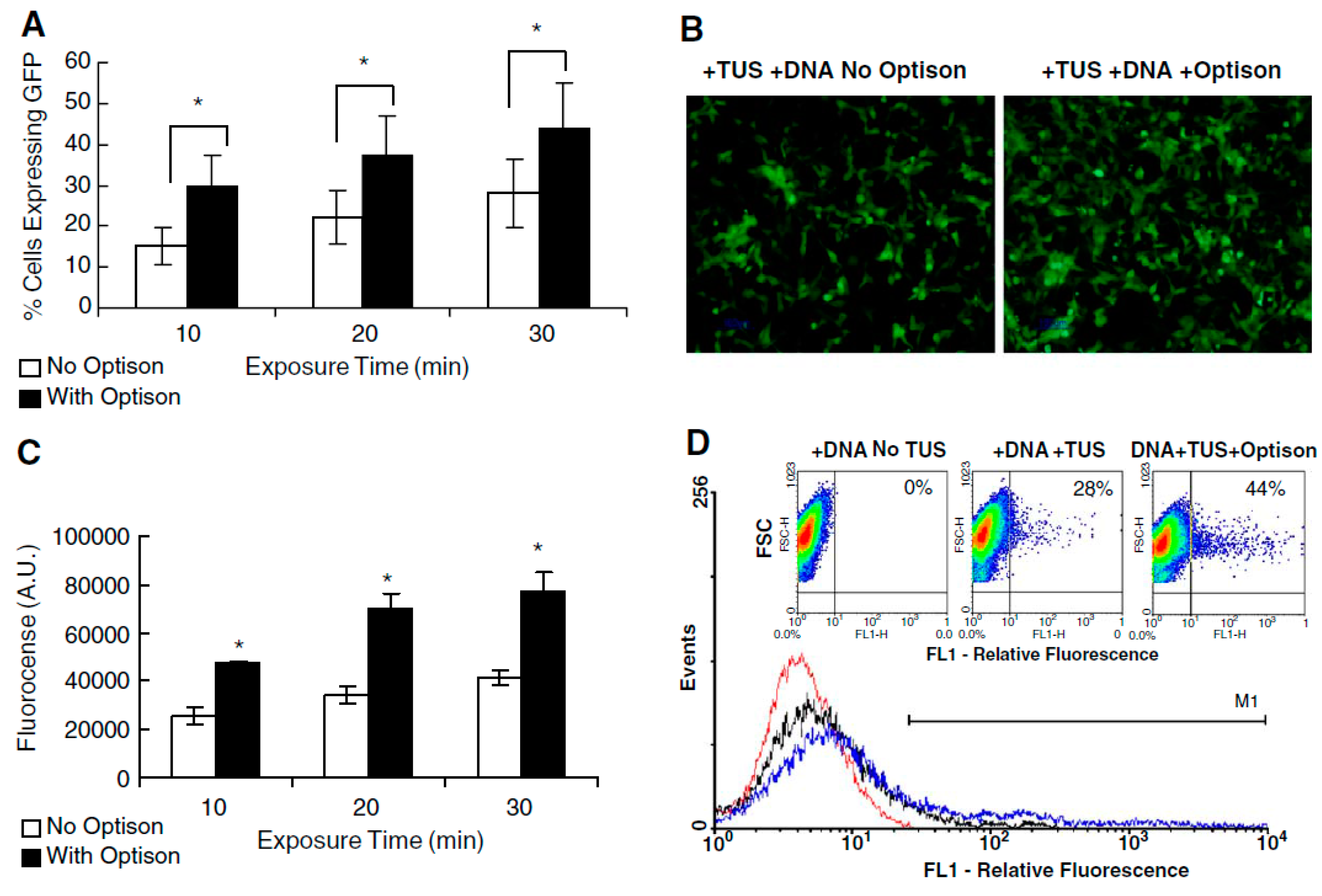
Most preclinical research focuses on tumor/cancer treatments of organs and tissues that are readily accessible by EMBs. The increasing knowledge of cellular and molecular mechanisms for human disease allows sonoporation to become a promising therapeutic alternative. Sonoporation for site-specific gene or drug delivery using EMBs has been extensively studied in cells in vitro. For example, Farokhzad et al. [38] pre-mixed plasmid DNA with Optison^® as the carrier, and applied a therapeutic ultrasound of 1 MHz, 30% duty cycle, spatial and temporal averaged intensity of 2 W/cm² for 0–30 min, to mediate gene delivery. Their results revealed that Optison^® microbubbles enhanced gene transfection by increasing the number of plasmids in the cells, and also by distributing the plasmids to more cells, without significant decrease in cell viability. Their results also demonstrated that Optison^® mainly affects the cytoplasmatic membrane, without interfering with intracellular DNA trafficking. As seen from Figure 5A, when DNA was first incubated with Optison^®, transfection efficiency was significantly higher than that achieved when therapeutical ultrasound (TUS) was applied alone for 10, 20, and 30 min (p < 0.05). This high transfection efficiency effect was also confirmed by fluorescent microscopy (Figure 5B), demonstrating an increase in the number of cells expressing green fluorescent protein (GFP) when adding Optison^®. The total fluorescence level was also significantly enhanced (p < 0.05) when Optison^® was pre-incubated with the DNA when compared to cells treated with TUS alone (Figure 5C). The results demonstrated that when US was applied for 30 min to cells, in the presence of Optison pre-incubated with DNA, the percent of cells expressing GFP increased from 28 ± 6% to 44 ± 8% (Figure 5D). From these studies it was also clear that the relative fluorescence enhancement indicates that more copies of plasmids entered cells.

Alter et al. [39] mixed phosphorodiamidate morpholino oligomers and plasmids with three different kinds of EMB spheres for their studies. Other approaches included therapeutic agents which were durably bound into the microbubble structure: plasmids were incorporated into microbubbles during the synthesis of albumin-shelled agents in an animal study. While the exact binding mechanism between the agent and the bubble was still elusive, the covalent bond was one possible stable linkage reported. It was discovered that ultrasound-mediated microbubble vascular disruption can enhance tumor responses to ionizing radiation in vivo [39]. Results indicate that there is a synergistic effect in vivo with combined single treatments of ultrasound-stimulated microbubble vascular perturbation with ionizing radiation inducing a more than10-fold greater cell destruction than with ionizing radiation alone. Thus, in vivo experiments with ultrasound combined with bubbles allow radiation doses to be decreased significantly to give a comparable effect. In order to ensure that microbubbles replenished the microvasculature between US pulses designed to cause microbubble disruption, the US pulse sequence for mouse treatments [40] was a 10% duty cycle within a 50-ms window every 2 s for a total active insonification time of 750 ms over 5 min, with an overall duty cycle of 0.25%. Microbubble disruption was carried out using a diagnostic ultrasound exposure of p = 570 kPa and a low mechanical index (0.76).

3.2. Thrombolysis and Stroke Treatment

Ischemic stroke is caused by the interruption of the blood flow to the brain. Stroke is a relatively common disease, particularly in senior citizens. Catheter–type ultrasound transducers to aid release of therapeutic drugs such as urokinase carried by EMBs have been used to increase the effectiveness of thrombolytic agents such as tissue plasminogen activator (t-PA); in contrast, controls treated with either ultrasound (490 KHz, spatial and temporal averaged intensity of 0.13 W/cm²) or microbubbles alone showed no effect in reducing thrombolysis. It is also known that the efficacy of t-PA decreases dramatically two hours after the stroke takes place. Intracranial clot lysis was also achieved in the arteries of swine [41] using thrombolytic agents with intravenous microbubbles assisted by therapeutic ultrasound. Alexandrov et al. [42] performed a pilot randomized clinical safety study for acute ischemic stroke involving sonothrombolysis using perfutren-lipid microbubbles administered intravenously (i.v.) and assisted by ultrasound excitation (2 MHz pulsed ultrasound with output power less than 720 mW measured by hydrophone; detailed information of US parameter was not reported in the literature). They reached the following conclusion: Perflutren microbubbles reached and permeated beyond intracranial occlusions with no increase in symptomatic intracranial hemorrhage after systemic thrombolysis. This suggested the feasibility of further microbubble dose-escalation studies, and the development of drug delivery to tissues with compromised perfusion.

3.3. Cancer Treatment

Numerous studies have been emerging for the treatment of cancer using sonoporation and targeted drug delivery (TDD) [38,39]. Compared with the serious adverse systemic side-effects and low efficacy associated with the use of chemotherapeutic drugs alone, TDD and sonoporation can reduce the required dose of chemotherapeutic drugs and improve their efficacy significantly. Heath et al. [43] delivered cisplatin and cetuximab with microbubbles into cancer-bearing mice. A significant reduction in tumor size was observed; an increased number of apoptotic cells was seen following the treatment, compared to that with chemotherapeutic agents alone. Using tumor-bearing mice as a model, Sorace et al. [44] studied the effects of TDD on the efficiency of drug uptake due to a systematic change of cell permeability by sonoporation. They reported that membrane permeability appeared to be dependent on ultrasound exposure parameters (acoustic amplitude, frequency, sonication time etc.); the resultant cancer cell death rate increased by over 50% compared with that from the chemotherapy treatment alone.

Brain diseases such as Parkinson’s and Alzheimer’s (AD) are difficult to treat clinically. One of hurdles is that neurons are tightly “sealed” by endothelial cells which form the so-called the blood–brain barrier (BBB). The BBB is a layer of tightly joined cells that line the blood vessels of the brain. It is used to prevent disease and preserve health by keeping harmful substances (such as toxins and infectious agents) from entering the brain. Unfortunately, this barrier also prevents certain drugs from reaching adequate concentrations in their targets within the brain, and there are limited options for circumventing the BBB to deliver them. The blood–brain barrier restricts the passage of substances from the bloodstream much more than do the endothelial cells in capillaries elsewhere in the body. Noninvasive, transient, and local blood-brain barrier disruption (BBBD) has been demonstrated following focused ultrasound exposure in animal models [45,46]. Most studies have combined low pressure amplitude and low time-averaged acoustic power burst sonications with intravascular injection of pre-formed micro-bubbles to produce BBBD without damage to neurons. For example, Samiotaki et al. [47] used pulsed US (center frequency 1.5 MHz, pulse length between 67 μs and 6.7 ms, and acoustic pressure amplitude ranging from 0.30 to 0.60 MPa) and T1-weighted magnetic resonance imaging (MRI) to quantify permeability changes. The BBB has been shown to reseal within a few hours of the US exposure. The MR image guided focused ultrasound beams allow precise anatomical targeting, as demonstrated by the delivery of several marker molecules in different animal models. This method may, in the future, have a significant impact on the diagnosis and treatment of central nervous system (CNS) disorders. Most notably, the delivery of chemotherapy agents (liposomal Doxorubicin and Herceptin) has been demonstrated in a rat model. Noninvasive, transient, and local image-guided blood-brain barrier disruption has been accomplished using focused ultrasound exposure with intravascular injection of microbubbles. The delivery of several marker molecules has been demonstrated in different animal models with minimal or no damage to the brain tissue.

Amyloid-β (Aβ) peptide has been connected with the pathogenesis of Alzheimer’s disease (AD). Ultrasound assistant cavitation bubbles have been shown to be able to overcome the BBB. By overcoming BBB, Leinenga et al. [48] applied repeated scanning ultrasound with bubbles to treat the mouse brain to remove Aβ without the need for any additional therapeutic agent such as anti-Aβ antibody. An integrated focused ultrasound system was used (TIPS, Philips Research, Eindhoven, The Netherlands), which consisted of an annular array transducer with a natural focus of 80 mm, a radius of curvature of 80 mm, a spherical shell of 80 mm with a central opening 31 mm in diameter, a 3D positioning system, and a programmable motorized system to move the ultrasound focus in the x and y planes to cover the entire brain area. A coupler mounted to the transducer was filled with degassed water and placed on the head of the mouse with ultrasound gel for coupling, to ensure propagation of the ultrasound to the brain. The focal zone of the array was an ellipse of about 1.5 mm × 1.5 mm × 12 mm. They optimized the ultrasound settings and used p = 0.7 MPa, 10-Hz pulse repetition frequency, 10% duty cycle, and 6-s sonication time per spot. This method may potentially open a new era in CNS targeted drug delivery.

4. Ultrasound Promotes Fluids’ Mixing within Microfluidic Devices

As shown in Figure 6a is a cylindrical Pyrex tube with inner and outer diameters of 34 mm and 36 mm, respectively, which was sealed at one end. An ultrasound transducer of radius b = 12 mm is placed at the other end [33]. The sealed end is referred to as the impingement surface, since the ultrasound waves impinge on this surface and are partially absorbed into the end-wall material. Different end-wall materials such acrylic or polyurethane were used for the impingement surface of 25 mm thick. The Pyrex tube was placed in a rectangular Pyrex tank, measuring 9  cm ×  9  cm × 7 cm. The cylindrical vessel was placed on a layer of 6 mm thick polyurethane, which was then placed on the 4 mm thick Pyrex bottom of the rectangular tank. This arrangement ensures negligible heat transfer through the bottom of the cylindrical vessel. The fluid velocity field in this case is generated by an ultrasound transducer along the axis of a cylindrical container of radius L as shown in Figure 6b. The transducer was excited at 2.25 MHz with a 10% duty cycle tune-burst voltage. The fluid flow field was measured using a planar particle image velocimetry (PIV) system, consisting of a double-pulsed Nd:YAG laser (New Wave, Solo PIV II15, New Wave Research, Inc., Fremont, CA, USA), a digital synchronizer, a cross correlation camera with 1376 × 1024 pixel resolution, a 7000 NAVITAR TV zoom lens (Navitar, Inc., Rochester, NY, USA), and the TSI Insight 3 G software (TSI Incorporated, Shoreview, MN, USA) for data processing. The fluid was seeded with 1.5 μm mean diameter Cospheric FMO Orange Fluorescent Microsphere (Cospheric LLC, Santa Barbara, CA, USA) seeding powder, with a density of 1.3 g/cm³. PIV images were taken in a vertical plane passing through the mid-point of the ultrasound transducer, with a time separation of between 2.5 and 30 ms between consecutive images in an image pair. Vector field frames were generated at a rate of 4.8 frames/s, which is a typical acoustic streaming field generated by a single ultrasound transducer [48]; it resembles the acoustic streaming field observed by Nowicki et al. [49]. One evident feature is the streaming velocity; its gradient becomes the greatest near the walls where the viscous boundaries locate, which is consistent with the numerical calculations recently reported by Marshall and Wu [6].

5. Conclusions

In this work, a brief review of the basic mathematic theory is provided to describe how boundary-associated acoustic streaming can be formed, and a DC fluid flow can be generated by an AC ultrasonic wave. Two necessary conditions for forming an acoustic streaming are: (1) Nonlinear wave propagation; and (2) A viscous fluid medium. There are two types microstreaming: Eckart streaming and Rayleigh streaming. The former takes place in a relative large fluid system; the dimension of the system is much greater than the wavelength of the ultrasound, while the latter occurs in a smaller system whose dimension is smaller than the wavelength. Rayleigh streaming is also called the boundary associated streaming; it usually happens in proximity of a boundary layer. Rayleigh streaming usually has the vortex-type flow. Figure 4 and Figure 5 contain its typical patterns. This review emphasizes the latter.

Acoustic streaming is used to promote fluid mixing in engineering applications. Recent development of the microfluidic devise make Rayleigh streaming broadly used in biomedical research. Sonoporation is a relatively new bio-technology; it takes advantage of Rayleigh streaming in the vicinity of an insulated microbubble. The microfluidic device, due to its small scale, just needs a small quantity of liquid cell sample for testing. The ultrasound source suitable for a microfluidic system is the surface acoustic wave of high frequency (for example about 20 MHz); therefore, the wavelength could be as small as submicron, which matches well with nanotechnology, and has a great potential to develop further in future. Reparable sonoporation is used in targeted drug delivery. The microfluidic device provides an ideal system for in vitro targeted drug delivery to test the efficacy of newly-developed drugs.

References

- Eckart, C. Vortices and streamings caused by sound waves. Phys. Rev. 1948, 73, 68–73. [Google Scholar] [CrossRef]
- Rayleigh, L. On the circulation of air observed in Kundt’s tube, and on some allied acoustic problem. Philos. Trans. 1883, 175, 1–21. [Google Scholar] [CrossRef]
- Lighthill, J. Acoustic streaming. J. Sound Vib. 1978, 61, 391–418. [Google Scholar] [CrossRef]
- Nyborg, W.L. Acoustic streaming near a boundary. J. Acoust. Soc. Am. 1958, 30, 329–339. [Google Scholar] [CrossRef]
- Kuznetsova, L.A.; Coakley, W.T. Applications of ultrasound streaming and radiation force in biosensors. Biosens. Bioelectron. 2007, 22, 1567–1577. [Google Scholar] [CrossRef] [PubMed]
- Marshall, J.; Wu, J. Acoustic streaming, fluid mixing, and particle transport by a Gaussian ultrasound beam in a cylindrical container. Phys. Fluids 2015, 27, 103601–1036021. [Google Scholar] [CrossRef]
- Pepe, J.; Ricon, M.; Wu, J. Experimental comparison of sonoporation and electroporation in cell transfection applications. Acoust. Res. Lett. Online 2004. [Google Scholar] [CrossRef]
- Wu, J.; Nyborg, W.L. Ultrasound, cavitation bubbles and their interaction with cells. Adv. Drug Deliv. Rev. 2008, 60, 1103–1116. [Google Scholar] [CrossRef] [PubMed]
- Crum, L.A. Measurements of the growth of air bubbles by rectified diffusion. J. Acoust. Soc. Am. 1980, 68, 203–211. [Google Scholar] [CrossRef]
- Gormley, G.; Wu, J. Observation of acoustic streaming near albunex spheres. J. Acoust. Soc. Am. 1998, 104, 3115–3118. [Google Scholar] [CrossRef]
- Rooney, J.A. Hemolysis near an ultrasonically pulsating gas bubble. Science 1970, 169, 869–871. [Google Scholar] [CrossRef] [PubMed]
- Rooney, J.A. Shear as a mechanism for sonically induced biological effects. J. Acoust. Soc. Am. 1972, 6, 1718–1724. [Google Scholar] [CrossRef]
- Elder, A.E. Cavitation microstreaming. J. Acoust. Soc. Am. 1959, 31, 54–64. [Google Scholar] [CrossRef]
- Inoue, H.; Arai, Y.; Kishida, T.; Shin-Ya, M.; Terauchi, R.; Nakagawa, S.; Saito, M.; Tsuchida, S.; Inoue, A.; Shirai, T.; et al. Sonoporation-mediated transduction of siRNA ameliorated experimental arthritis using 3 MHz pulsed ultrasound. Ultrasonics 2014, 54, 874–881. [Google Scholar] [CrossRef] [PubMed]
- van Wamel, A.; Bouakaz, A.; Versluis, M.; de Jong, N. Micromanipulation of endothelial cells: Ultrasound-microbubble-cell interaction. Ultrasound Med. Biol. 2004, 30, 1255–1258. [Google Scholar] [CrossRef] [PubMed]
- Meijering, B.D.M.; Juffermans, L.J.M.; van Wamel, A.; Henning, R.H.; Zuhorn, I.S.; Emmer, M.; Versteilen, A.M.G.; Paulus, W.J.; van Gilst, W.H.; Kooiman, K.; et al. Ultrasound and microbubble-targeted delivery of macromolecules is regulated by induction of endocytosis and pore formation. Circ. Res. 2009, 104, 679–687. [Google Scholar] [CrossRef] [PubMed]
- Frenkel, V. Ultrasound mediated delivery of drugs and genes to solid tumors. Adv. Drug Deliv. Rev. 2008, 60, 1193–1208. [Google Scholar] [CrossRef] [PubMed]
- Guzmán, H.; Nguyen, D.; Khan, S.; Prausnitz, M. Ultrasound-mediated disruption of cell membranes. II. Heterogeneous effects on cells. J. Acoust. Soc. Am. 2001, 110, 597–606. [Google Scholar] [CrossRef] [PubMed]
- Karshafian, R.; Samac, S.; Bevan, P.; Burns, P. Microbubble mediated sonoporation of cells in suspension: Clonogenic viability and influence of molecular size on uptake. Ultrasonics 2010, 50, 691–697. [Google Scholar] [CrossRef] [PubMed]
- Wu, J.; Ross, J.P.; Chiu, J.-F. Reparable Sonoporation Generated by Microstreaming. J. Acoust. Soc. Am. 2001, 111, 1460–1464. [Google Scholar] [CrossRef]
- Wu, J. Theoretical study on shear stress generated by microstreaming surrounding contrast agents attached to living cells. Ultrasound Med. Biol. 2002, 28, 125–129. [Google Scholar] [CrossRef]
- Peruzzi, G.; Massimo, C. Perspectives on cavitation enhanced endotherlia layer permeability. Colloids Surf. B Biointerfaces 2018. [Google Scholar] [CrossRef] [PubMed]
- Ma, D.; Wu, J. Biofilm mitigation by drug (gentamicin) loaded liposomes promoted by pulsed ultrasound. J. Acoust. Soc. Am. 2016. [Google Scholar] [CrossRef] [PubMed]
- Ma, D.; Adam Green, A.M.; Willsey, G.G.; Marshall, J.S.; Wargo, M.J.; Wu, J. Effects of acoustic streaming of moderate pulsed ultrasound promoting bacteria eradication of biofilms using drug loading liposomes. J. Acoust. Soc. Am. 2015, 138, 1043–1051. [Google Scholar] [CrossRef] [PubMed]
- Wiklund, M.; Green, R.; Ohlin, M. Acoustofluidics 14: Applications of acoustic streaming in microfluidic devices. Lab Chip 2012, 12, 2438–2451. [Google Scholar] [CrossRef] [PubMed]
- Leslie, Y.; Yeo, L.Y.; Friend, J.R. Surface acoustic wave microfluidics. Annu. Rev. Fluid Mech. 2014, 46, 379–406. [Google Scholar]
- Ding, X.; Li, P.; Lin, S.C.; Stratton, Z.S.; Nama, N.; Guo, F.; Slotcavage, D.; Mao, X.; Shi, J.; Costanzo, F.; et al. Surface acoustic wave microfluidics. Lab Chip 2013, 13, 3626–3649. [Google Scholar] [CrossRef] [PubMed] [Green Version]
- Li, H.; Friend, J.R.; Yeo, L.Y. Surface acoustic wave concentration of particle and bioparticle suspensions. Biomed. Microdevices 2007, 9, 647–656. [Google Scholar] [CrossRef] [PubMed]
- Ding, X.; Lin, S.-C.S.; Kiraly, B.; Yue, H.; Li, S.; Chiang, I.-K.; Stephen, S.J.; Benkovic, J.; Huang, T.J. On-chip manipulation of single microparticles, cells, and organisms using surface acoustic waves. PNAS 2012, 109, 11105–11109. [Google Scholar] [CrossRef] [PubMed] [Green Version]
- Meng, L.; Cai, F.; Jin, Q.; Niu, L.; Jiang, C.; Wang, Z.; Wu, J.; Zheng, H. Acoustic aligning and trapping of microbubbles in an enclosed PDMS microfluidic device. Sens. Actuators B Chem. 2011, 160, 1599–1605. [Google Scholar] [CrossRef]
- Meng, L.; Cai, F.; Wu, J.; Zheng, H. Precise and programmable manipulation of microbubbles by two-dimensional standing surface acoustic waves. Appl. Phys. Lett. 2012, 100, 173701. [Google Scholar] [CrossRef]
- Meng, L.; Deng, Z.; Niu, L.; Li, F.; Yan, F.; Wu, J.; Cai, F.; Zheng, H. A disposable microfluidic device for controlled drug release from thermal-sensitive liposomes by high intensity focused ultrasound. Theranostics 2015, 5, 1203–1213. [Google Scholar] [CrossRef] [PubMed]
- Green, A.; Marshall, J.S.; Ma, D.; Wu, J. Acoustic streaming and thermal instability of flow generated by ultrasound in a cylindrical container. Phys. Fluids 2016, 28, 104105. [Google Scholar] [CrossRef]
- Wu, J. Handbook of Contemporary Acoustics and Its Application; World Scientific Co.: Hackensack, NJ, USA, 2016; p. 327. [Google Scholar]
- Riley, K.F.; Hobson, M.P. Solution methods for PDEs. In Essential Mathematical Methods; Cambridge University Press: New York, NY, USA, 2011; pp. 421–479. [Google Scholar]
- Lei, J.; Glynne-Jones, P.; Hill, M. Acoustic streaming in the transducer plane in ultrasonic particle manipulation devices. Lab Chip 2013, 13, 2133. [Google Scholar] [CrossRef] [PubMed] [Green Version]
- Duvshani-Eshet, M.; Adam, D.; Machluf, M. The effects of albumin-coated microbubbles in DNA delivery mediated by therapeutic ultrasound. J. Control. Release 2006, 112, 156–166. [Google Scholar] [CrossRef] [PubMed]
- Farokhzad, O.C.; Cheng, J.; Teply, B.A.; Sherifi, I.; Jon, S.; Kantoff, P.W. Targeted nanoparticle-aptamer bioconjugates for cancer chemotherapy in vivo. Proc. Natl. Acad. Sci. USA 2006, 103, 6315–6320. [Google Scholar] [CrossRef] [PubMed] [Green Version]
- Alter, J.; Sennoga, C.A.; Lopes, D.M.; Eckersley, R.J.; Wells, D. Microbubble stability is a major determinant of the efficiency of ultrasound and microbubble mediated in vivo gene transfer. Ultrasound Med. Biol. 2009, 35, 976–984. [Google Scholar] [CrossRef] [PubMed]
- Fujii, H.; Sun, Z.; Li, S.H.; Wu, J.; Fazel, S.; Weisel, R.D.; Rakowski, H.; Lindner, J.; Li, R.K. Ultrasound-targeted gene delivery induces angiogenesis after a myocardial infarction in mice. J. Am. Coll. Cardiol. 2009, 2, 869–879. [Google Scholar] [CrossRef] [PubMed]
- Czarnota, G.J.; Karshafian, R.; Burns, P.N.; Wong, S.; Mahrouki, A.A.; Lee, J.W.; Caissie, A.; Tran, W.; Kim, C.; Furukawa, M.; et al. Tumor radiation response enhancement by acoustical stimulation of the vasculature. PNAS 2012, 9, E2033–E2041. [Google Scholar] [CrossRef] [PubMed]
- Alexandrov, A.V.; Mikulik, R.; Ribo, M.; Sharma, V.K.; Lao, A.Y.; Tsivgoulis, G.; Sugg, R.M.; Barreto, A.; Sierzenski, P.; Malkoff, M.D.; et al. A Pilot randomized clinical safety study of sonothrombolysis augmentation with ultrasound-activated perflutren-lipid microspheres for acute ischemic stroke. Stroke 2008, 39, 1464–1469. [Google Scholar] [CrossRef] [PubMed]
- Heath, C.H.; Sorace, A.; Knowles, J.; Rosenthal, E.; Hoyt, K. Microbubble therapy enhances anti-tumor properties of cisplatin and cetuximab in vitro and in vivo. Otolaryngol. Head Neck Surg. 2012, 146, 938–945. [Google Scholar] [CrossRef] [PubMed]
- Sorace, A.G.; Warram, J.M.; Umphrey, H.; Hoyt, K. Microbubble-mediated ultrasonic techniques for improved chemotherapeutic delivery in cancer. J. Drug Target. 2012, 20, 43–54. [Google Scholar] [CrossRef] [PubMed]
- Tachibana, K.; Tachibana, S. Emerging technologies using ultrasound for drug delivery. In Emerging Therapeutic Ultrasound; Wu, J., Nyborg, W.L., Eds.; World Scientific Co.: Hackensack, NJ, USA, 2007. [Google Scholar]
- Culp, W.C.; Porter, T.R.; Lowery, J.; Xie, F.; Roberson, P.K.; Marky, L. Intracranial clot lysis with intravenous microbubbles and transcranial ultrasound in swine. Stroke 2004, 35, 2407–2411. [Google Scholar] [CrossRef] [PubMed]
- Samiotaki, G.; Konofagou, E.E. Dependence of the reversibility of focused-ultrasound-induced blood–brain barrier opening on pressure and pulse length in vivo. IEEE Trans. Ultrason. Ferroelectr. Freq. Control 2013, 60, 2257–2265. [Google Scholar] [CrossRef] [PubMed]
- Leinenga, G.; Gotz, J. Scanning ultrasound removes Amylaid-β and restores memory in an Alzheimer’s disease mouse model. Sci. Transl. Med. 2015, 7, 278ra33. [Google Scholar] [CrossRef]
- Nowicki, A.; Kowaleski, T.; Worjeik, J. Estimation of acoustic streaming: Theoretical model, Doppler measurements and optical visualization. Eur. J. Ultrasound 1998, 7, 73–81. [Google Scholar] [CrossRef]
Figure 1.
Acoustic streaming generated by a finite acoustic beam in a closed tube. Reproduced with permission from [34].
Figure 2.
Two rigid planes separated by a distance H.
Figure 3.
(a) Acoustic streaming in a standing wave: the standing wave’s spatial period is twice that of vortex-rings of acoustic streaming; (b) acoustic streaming pattern between (−λ/4) on the left of an antinode to λ/4 on the right of the antinode. Note the streaming directions within viscous boundary layers, are counterclockwise directions of those outside the boundary. Reproduced with permission from [34].
Figure 4.
A photo of the microstreaming generated by a 10 EMB located at an antinode of a standing wave of 160 kHz ultrasound. Reproduced with permission from [10].
Figure 5.
The effects of Optison® on therapeutic ultrasound (TUS) transfection using pIRES-EGFP-BHK, a polymerase cellular promoters, cells were treated with 1 MHz TUS at 30% DC and 2 W/ with or without Optison®. (A) Effect of Optison®; (B) Fluorescent micrographs of cells expressing green fluorescent protein (GFP) 24 h post TUS transfection for 30 min with or without Optison®. (C) Effects of Optison® on total GFP expression post TUS. (D) Fluorescence-activated cell sorting (FACS) analysis of cells 24 h post TUS transfection for 30 min. FACS Dot-plot showing cell size (FSC) vs. green fluorescence (FL1) and percentage of the number of cells with fluorescence greater than the control * p < 0.05. Reproduced with permission from [37].
© 2018 by the author. Licensee MDPI, Basel, Switzerland. This article is an open access article distributed under the terms and conditions of the Creative Commons Attribution (CC BY) license (http://creativecommons.org/licenses/by/4.0/).
Share and Cite
MDPI and ACS Style
Wu, J. Acoustic Streaming and Its Applications. Fluids 2018, 3, 108. https://0-doi-org.brum.beds.ac.uk/10.3390/fluids3040108
AMA Style
Wu J. Acoustic Streaming and Its Applications. Fluids. 2018; 3(4):108. https://0-doi-org.brum.beds.ac.uk/10.3390/fluids3040108
Chicago/Turabian StyleWu, Junru. 2018. "Acoustic Streaming and Its Applications" Fluids 3, no. 4: 108. https://0-doi-org.brum.beds.ac.uk/10.3390/fluids3040108