Teaching Fluid Mechanics and Thermodynamics Simultaneously through Pipeline Flow Experiments

Department of Chemical Engineering, University of Waterloo, Waterloo, ON N2L 3G1, Canada
Fluids 2019, 4(2), 103; https://0-doi-org.brum.beds.ac.uk/10.3390/fluids4020103
Submission received: 12 May 2019
/
Revised: 26 May 2019
/
Accepted: 28 May 2019
/
Published: 1 June 2019
(This article belongs to the Special Issue Teaching and Learning of Fluid Mechanics)
Abstract
:Entropy and entropy generation are abstract and illusive concepts for undergraduate students. In general, students find it difficult to visualize entropy generation in real (irreversible) processes, especially at a mechanistic level. Fluid mechanics laboratory can assist students in making the concepts of entropy and entropy generation more tangible. In flow of real fluids, dissipation of mechanical energy takes place due to friction in fluids. The dissipation of mechanical energy in pipeline flow is reflected in loss of pressure of fluid. The degradation of high quality mechanical energy into low quality frictional heat (internal energy) is simultaneously reflected in the generation of entropy. Thus, experiments involving measurements of pressure gradient as a function of flow rate in pipes offer an opportunity for students to visualize and quantify entropy generation in real processes. In this article, the background in fluid mechanics and thermodynamics relevant to the concepts of mechanical energy dissipation, entropy and entropy generation are reviewed briefly. The link between entropy generation and mechanical energy dissipation in pipe flow experiments is demonstrated both theoretically and experimentally. The rate of entropy generation in pipeline flow of Newtonian fluids is quantified through measurements of pressure gradient as a function of flow rate for a number of test fluids. The factors affecting the rate of entropy generation in pipeline flows are discussed.
1. Introduction
Fluid mechanics, that is, the study of motion of fluids and forces in fluids, is relatively a less abstract subject as compared with thermodynamics. Students find it relatively easy to visualize and understand the motion of fluids and forces in fluids. For example, it is not difficult to convey to the students fluid mechanics concepts such as pressure, pressure distribution, viscosity, velocity distribution, velocity gradient, shear and normal stresses, mechanical energy dissipation and pressure loss in flow of fluids due to friction, etc. Most fluid mechanics quantities are directly measurable. For example, instruments are available to directly measure pressure or pressure drop, flow rate, local velocity, shear and normal stresses, etc. Thermodynamics, on the other hand, is a very abstract subject. Concepts such as entropy and entropy generation in real processes are illusive for students. There are no instruments available which can be used to directly measure entropy and entropy generation in real processes.
It is a well-known fact that students learn and understand concepts better and with relative ease through experiential learning. It is appropriate to quote here a famous Chinese saying credited to the Chinese philosopher Confucius, “I hear and I forget; I see and I remember; I do and I understand”. To that end, the undergraduate laboratory experiments can play a very important role in providing experiential learning of concepts and theory to students.
In most undergraduate engineering programs (chemical, mechanical, civil, etc.) students are taught fluid mechanics through in-class instruction and laboratory experiments. In a typical undergraduate fluid mechanics laboratory, the students are required to do pipeline flow experiments involving measurement of pressure loss as a function of flow rate for different diameter pipes. The flow rate is measured with the help of a flowmeter and the pressure drop is measured with the help of pressure transducers. The test fluid is usually water and the experiments are carried out at room temperature. From pressure drop vs. flow rate experimental data, friction factor vs. Reynolds number data are calculated and compared with the available theoretical and empirical relations. What is completely missing in the undergraduate fluid mechanics experiments is the link between the pipeline flow experiments and the second law of thermodynamics, that is, entropy and entropy generation in pipeline flows. In order to appreciate and understand the second law of thermodynamics, it is important for students to be able to relate the directly measureable quantities like pressure loss in pipeline flow to entropy generation in real flows.
The main objectives of this article are: (1) to briefly review the background in fluid mechanics and thermodynamics related to pressure loss, mechanical energy dissipation, and entropy generation in real flows; (2) to demonstrate the link between mechanical energy dissipation and entropy generation in real flows; (3) to carry out experimental work to determine friction factor as a function of Reynolds number and entropy generation rate as a function of fluid velocity in flow of emulsion-type test fluids in different diameter pipelines; and (4) to explain mechanistically the cause of entropy generation in real flows.
2. Background
2.1. Fluid Mechanics
Consider flow of a fluid through a stationary control volume. The macroscopic balance of any entity (mass, momentum, energy) over the control volume can be expressed as:
The application of the entity balance equation, Equation (1), to mass gives the following integral equation [1,2]:
where is the fluid density, is the unit outward normal to the control surface, is the fluid velocity vector, is the control surface area, is the time, is the volume of the control volume, the cyclic double integral is the surface integral over the entire control surface, and the cyclic triple integral is the volume integral over the entire control volume. It should be noted that the surface integral is the net outward flow of mass across the entire control surface. The volume integral is the rate of accumulation of mass within the entire control volume (assumed to be fixed and non-deforming). For a control volume with one inlet and one outlet, the macroscopic or integral mass balance equation, Equation (2), under steady state condition, reduces to:
where is the fluid velocity, is the cross-section area of inlet or outlet opening, and is the mass flow rate. The subscript 1 indicates inlet variables and the subscript 2 indicates outlet variables.
The application of the entity balance equation, Equation (1), to linear momentum gives the following integral equation [1,2]:
where is the force vector. Equation (4) is often referred to as momentum theorem [1]. The surface integral is the net outward flow of linear momentum across the entire control surface. The volume integral is the rate of accumulation of linear momentum within the entire control volume (assumed to be fixed and non-deforming). The momentum balance equation, Equation (4), is a vector equation. In Cartesian coordinates, the vector momentum balance equation can be written as three scalar equations:
where and are velocity and force components in directions. For a control volume with one inlet and one outlet, the macroscopic or integral momentum balance equations, Equations (5)–(7), under steady state condition, reduce to:
Using mass balance, Equation (3), Equations (8)–(10) can be further simplified as:
Note that we are assuming velocity profiles are uniform at inlet and outlet of the control volume.
The application of the entity balance equation, Equation (1), to mechanical energy gives the following integral equation assuming frictionless flow [1,2]:
where is the potential energy per unit mass, is the kinetic energy per unit mass, is the pressure, and is the rate of shaft work. The surface integral is the net outward flow of mechanical energy (including flow work) across the entire control surface. The volume integral is the rate of accumulation of mechanical energy within the entire control volume (assumed to be fixed and non-deforming). For a control volume with one inlet and one outlet, the macroscopic mechanical energy balance equation for frictionless flow, Equation (14), under steady state condition, reduces to:
Using mass balance, Equation (3), Equation (15) can be further simplified as:
Note that mechanical energy is conserved only in frictionless flows. In real flows, however, mechanical energy is not conserved as mechanical energy dissipation occurs due to friction in fluids. The mechanical energy loss due to friction in real flows can be treated as negative generation (destruction) in entity balance equation, Equation (1). Thus, Equation (16) can be modified as [2]:
where is the rate of mechanical energy dissipation due to friction in fluid. Equation (17) assumes that the velocity profiles are uniform at inlet and outlet of the control volume. Furthermore any work due to viscous effects (shear stresses and viscous normal stresses) at the control surface is assumed to be negligible.
2.2. Thermodynamics
The first law of thermodynamics is simply the principle of conservation of energy. When applied to a control volume, it indicates that that the rate of accumulation of total energy inside the control volume is equal to the net rate of total energy addition to the control volume. Equation (1) is applicable to total energy as the entity with no generation. For a stationary control volume (fixed and non-deforming control volume), the first law of thermodynamics can be expressed as [1]:
where is the specific total energy (total energy per unit mass) of fluid and is the rate of heat transfer. The specific total energy includes internal energy, kinetic energy and potential energy, that is, , where is the specific internal energy. The work associated with shear stress and viscous portion of normal stress at the control surface is assumed to be zero [1]. The surface integral is the net outward flow of total energy (including flow work) across the entire control surface. The volume integral is the rate of accumulation of total energy within the entire control volume.
For a control volume with one inlet and one outlet, the macroscopic total energy balance (first law of thermodynamics), Equation (18), under steady state condition, reduces to:
Using mass balance, Equation (3), Equation (19) can be further simplified as:
As
where is acceleration due to gravity, is elevation and is specific enthalpy of fluid given as: , Equation (20) could also be written as:
For reversible (frictionless) flows, it can be readily shown that
Upon substitution of from Equation (23) into Equation (22), the mechanical energy balance equation for frictionless flow, Equation (16), is recovered.
The second law of thermodynamics states that all irreversible (real) processes are accompanied by entropy generation in the universe [3]. For flow through a stationary control volume, the entropy generation rate ( in the universe can be expressed as:
where is the entropy per unit mass of fluid, is the rate of heat transfer to control volume from ith heat reservoir at an absolute temperature of , the subscripts and refer to control volume and surroundings, respectively. The equality in Equation (24) is valid for any reversible (frictionless) process and the inequality is valid for all irreversible processes. The surface integral is the net outward flow of entropy across the entire control surface. The volume integral is the rate of accumulation of entropy within the entire control volume (assumed to be fixed and non-deforming).
For a control volume with one inlet and one outlet, Equation (24), under steady state condition, reduces to:
Using mass balance, Equation (3), Equation (25) can be further simplified as:
2.3. Steady Flow in a Pipe
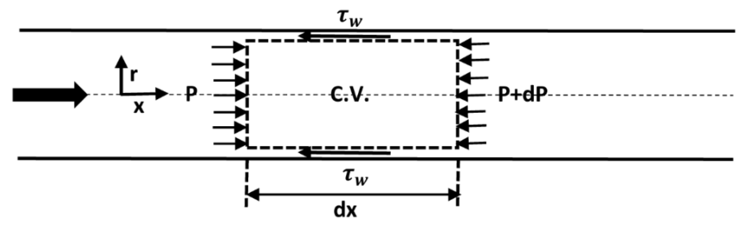
Consider steady flow of an incompressible fluid in a cylindrical pipe of uniform diameter (see Figure 1). From mass balance,
As and are constant, the velocity is constant,
From momentum balance, Equation (11):
Now consider force balance over a differential control volume of length as shown in Figure 1:
where is the wall shear stress, is the pipe internal diameter, and . Equation (30) leads to:
Upon rearrangement, Equation (31) gives
where is the pipe radius. Equation (32) can also be applied to any radial position as:
where is any radial position in the pipe. From Equations (32) and (33), it follows that:
Equation (34) describes the variation of shear stress with the radial position. The shear stress varies linearly with the radial position.
Using macroscopic mechanical energy balance, Equation (17), it can be readily shown that for steady incompressible flow in a horizontal pipe of uniform diameter:
where is the length of the pipe. The rate of mechanical energy loss can further be expressed in terms of a friction factor () defined as:
where is the average velocity in the pipe. Upon substitution of from Equation (32) into Equation (36), we get
From Equations (35) and (37), it follows that the mechanical energy loss per unit mass of fluid is:
From Equation (38), it follows that the mechanical energy loss per unit length per unit mass of fluid is:
In order to calculate the mechanical energy loss in pipeline flows, the value of friction factor is required.
In laminar flow of Newtonian fluids , friction factor is related to Reynolds number through the following theoretical relationship [1,4]:
where the Reynolds number is defined as:
In turbulent flow of Newtonian fluids, friction factor is a function of Reynolds number and relative roughness of pipe . For hydraulically smooth pipes , the friction factor depends only on in turbulent regime. The following semi-empirical equation, often referred to as von Karman–Nikuradse equation, describes the turbulent behavior of Newtonian fluids in smooth pipes very well [1]:
The von Karman–Nikuradse equation is not explicit in friction factor. A number of explicit relations are available in the literature. One of the popular ones is the Blasius friction factor equation for turbulent flow of Newtonian fluids in smooth pipes [4]:
Equation (43) is accurate over a Reynolds number range of . For turbulent flow in rough pipes, the following Colebrook equation [5,6] is widely accepted:
This Colebrook equation is implicit in friction factor. A number of explicit relations are available in the literature for turbulent flow of Newtonian fluids in rough pipes [7,8,9]. An explicit equation which is very accurate for turbulent flow of Newtonian fluids in rough pipes is as follows:
This equation was originally proposed by Zigrang and Sylvester [10].
2.4. Entropy Generation in Steady Flow in a Pipe
In flow of real fluids, the dissipation of mechanical energy, and hence loss of pressure, is simultaneously reflected in the generation of entropy [11,12]. Consequently, the pipeline flow experiments performed by undergraduate students in the fluid mechanics laboratory can also be used as a tool to teach the second law of thermodynamics which states that all real processes are accompanied by generation of entropy in the universe.
For steady flow in a pipe with no heat transfer, Equation (26) reduces to:
There is no entropy generation in the surroundings. All the entropy is generated within the fluid inside the pipe and the rate of entropy generation is the net rate of increase in entropy of the flowing stream.
We can now relate entropy change of the fluid stream to other variables. For pure substances, the relationship between entropy and other state variables is given as [3]:
where is the absolute temperature. From the first law of thermodynamics, Equation (22), the enthalpy change is zero in the absence of heat transfer and shaft work for steady flow in a horizontal pipe of uniform diameter. Consequently, Equation (48) reduces to:
Assuming incompressible flow and constant temperature, Equation (49) upon integration gives:
Strictly speaking, the temperature is expected to rise somewhat in adiabatic flow due to frictional heating. However, the temperature rise is usually very small in pipeline flow experiments conducted in the undergraduate fluid mechanics laboratory. From Equations (47) and (50), it follows that:
The subscript “CV” has been removed from for the sake of simplicity. We can also express the rate of entropy generation in a pipe on a unit length basis as:
where is the rate of entropy generation per unit length of the pipe. From Equations (37) and (52), it can be readily shown that:
In laminar flow, the friction factor is given by Equation (40). Consequently, Equation (53) yields:
Thus entropy generation rate per unit length of pipe in steady laminar flow of a Newtonian fluid is directly proportional to fluid viscosity and square of average velocity in the pipe.
In turbulent flow of a Newtonian fluid in hydraulically smooth pipe, Equations (43) and (53) give the flowing expression for entropy generation rate per unit length of pipe:
In turbulent flow, the entropy generation rate per unit length of pipe also depends on pipe diameter and fluid density, in addition to viscosity and fluid velocity dependence. Although the viscosity dependence of in turbulent flow is less severe in comparison with laminar flow, the velocity dependence is stronger in turbulent flow.
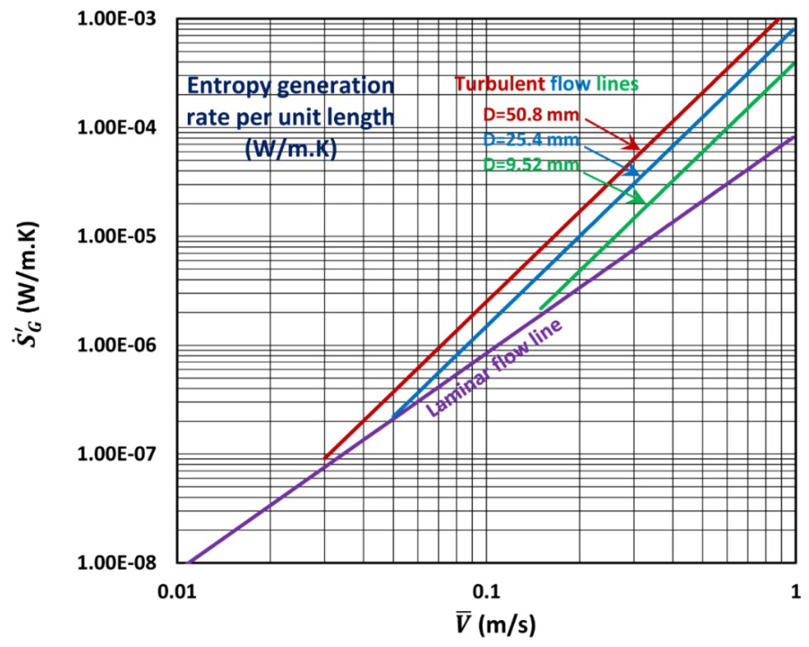
Figure 2 shows the plots of on a log-log scale for laminar and turbulent flows generated from Equations (54) and (55), respectively. The fluid properties used in the equations are: . The temperature used is 298.15 K. A single line of slope 2 is obtained for laminar regime regardless of the pipe diameter. The entropy generation rate per unit length of the pipe increases linearly with the increase in average velocity in the pipe. A family of parallel lines of slope 2.75 is obtained for the turbulent regime. The line shifts upward towards higher entropy generation rate with the increase in the pipe diameter.
3. Experimental Work
3.1. Apparatus
A flow rig consisting of five different diameter pipeline test sections (stainless steel seamless tubes, hydraulically smooth) was designed and constructed. The pipelines were installed horizontally. Table 1 gives the dimensions of the test sections. The test fluid was circulated through the pipeline test sections, one at a time, using a centrifugal pump. An electromagnetic flow meter was used to measure the flow rate of a fluid circulated through the test section. The pressure drop in a pipeline test section was measured using pressure transducers covering a broad range of pressure drops. The pressure drop as a function of flow rate was recorded by a computer data acquisition system. The experiments were carried out at a constant temperature of 25 °C.
3.2. Test Fluids
The test fluids used were surfactant-stabilized oil-in-water (O/W) emulsions. The viscosity of the test fluid was increased by increasing the oil concentration of the emulsion. Table 2 summarizes the viscosity and density data of the test fluids at 25 °C.
4. Results and Discussion
4.1. Fluid Mechanics Experiments
The experimental data obtained from pipeline flow experiments consist of pressure drop (over a known length of pipe) versus flow rate for different diameter pipes. From pressure drop versus flow rate data, friction factor is calculated from Equation (37), re-written as:
where the average velocity is obtained from:
Here is the volumetric flow rate of fluid. The Reynolds is calculated from the defining relation, Equation (41), re-written as:
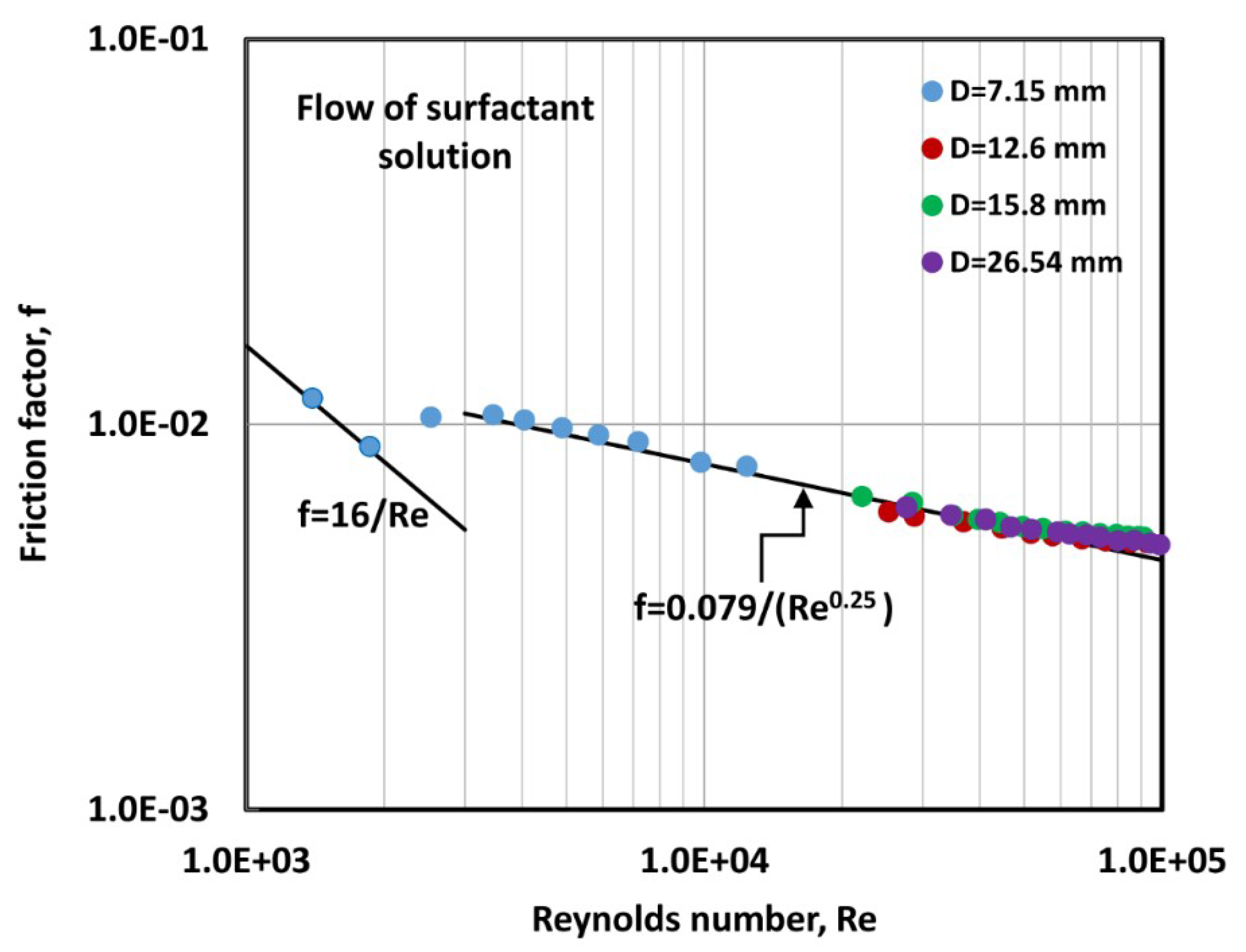
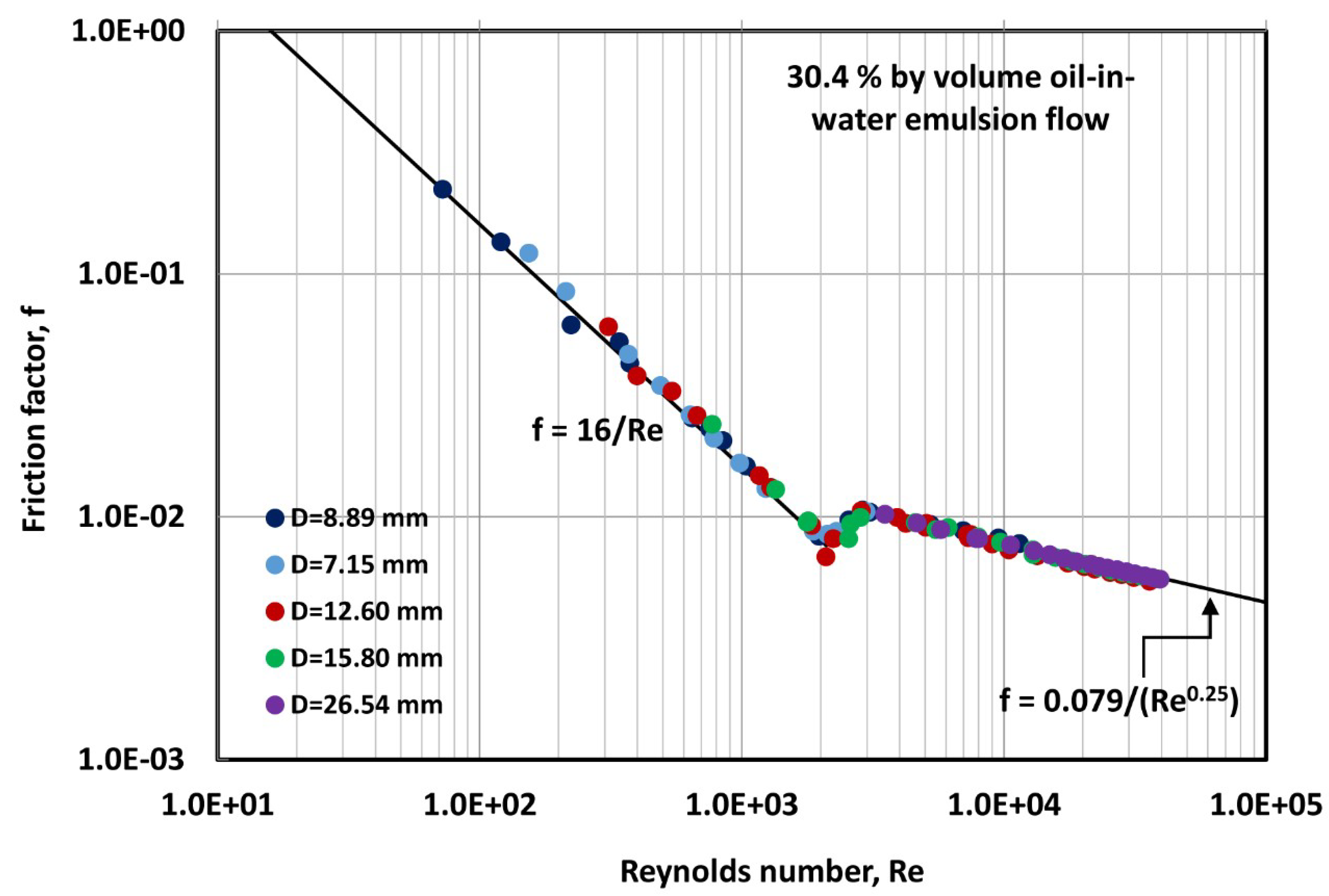
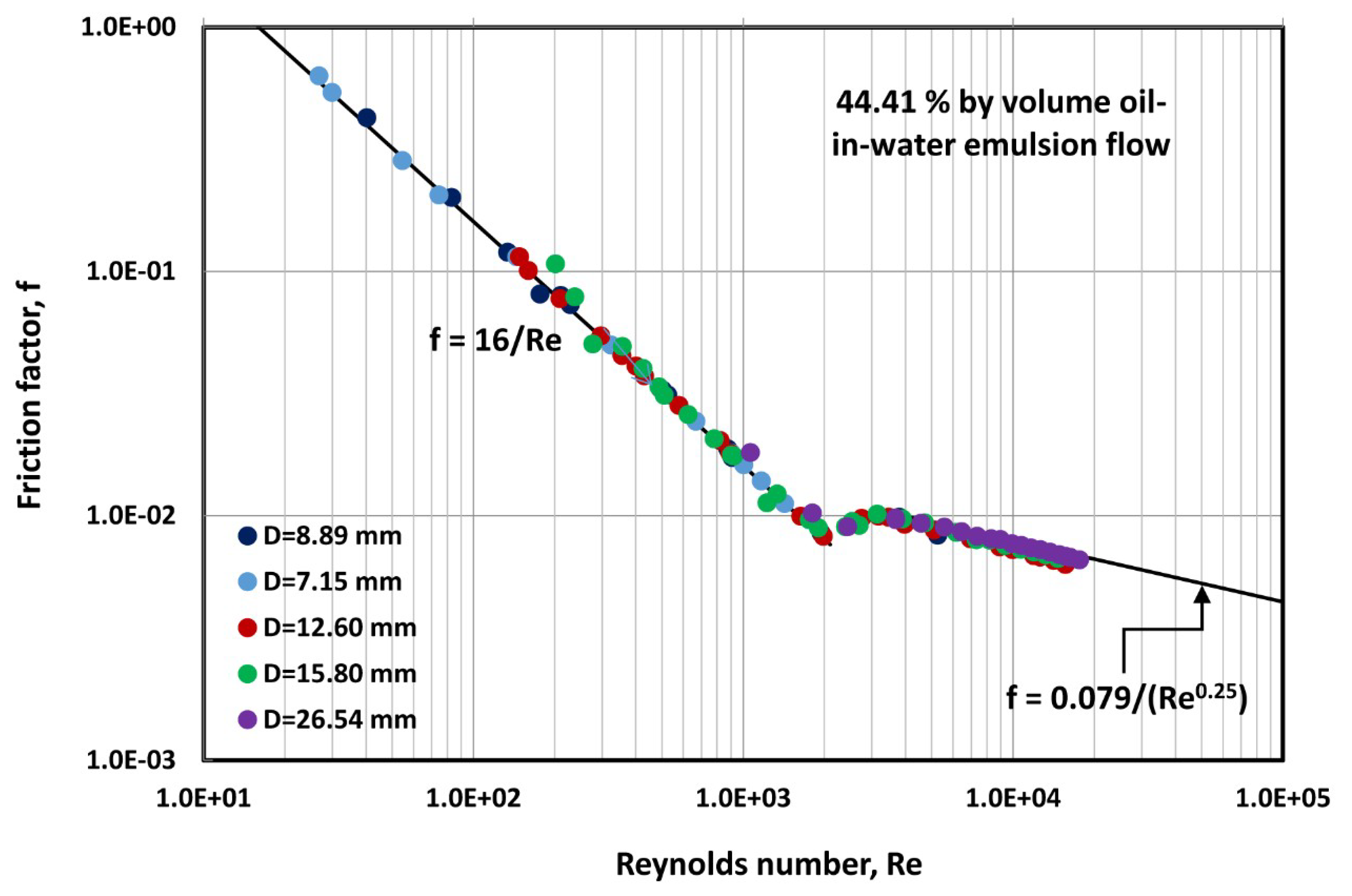
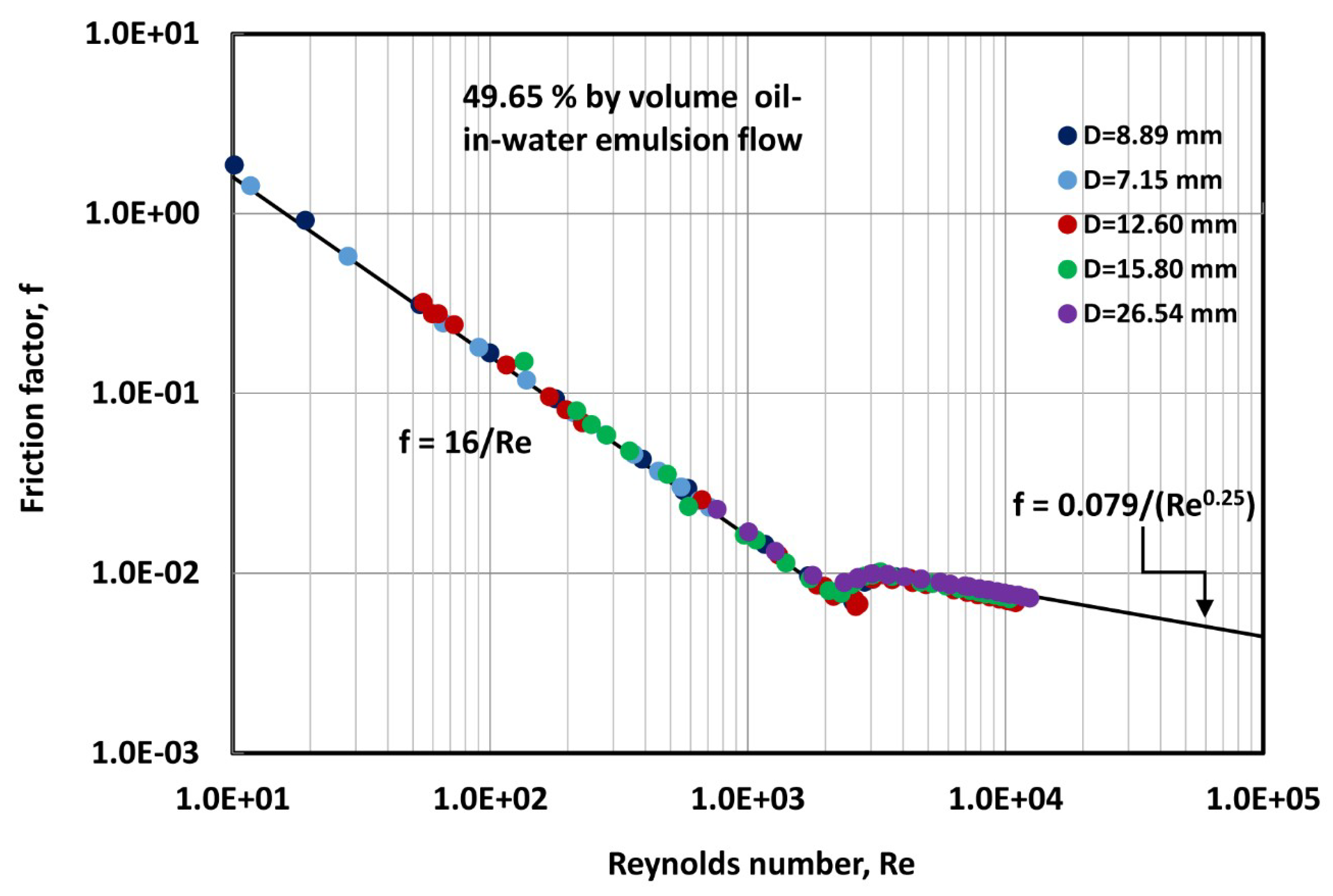
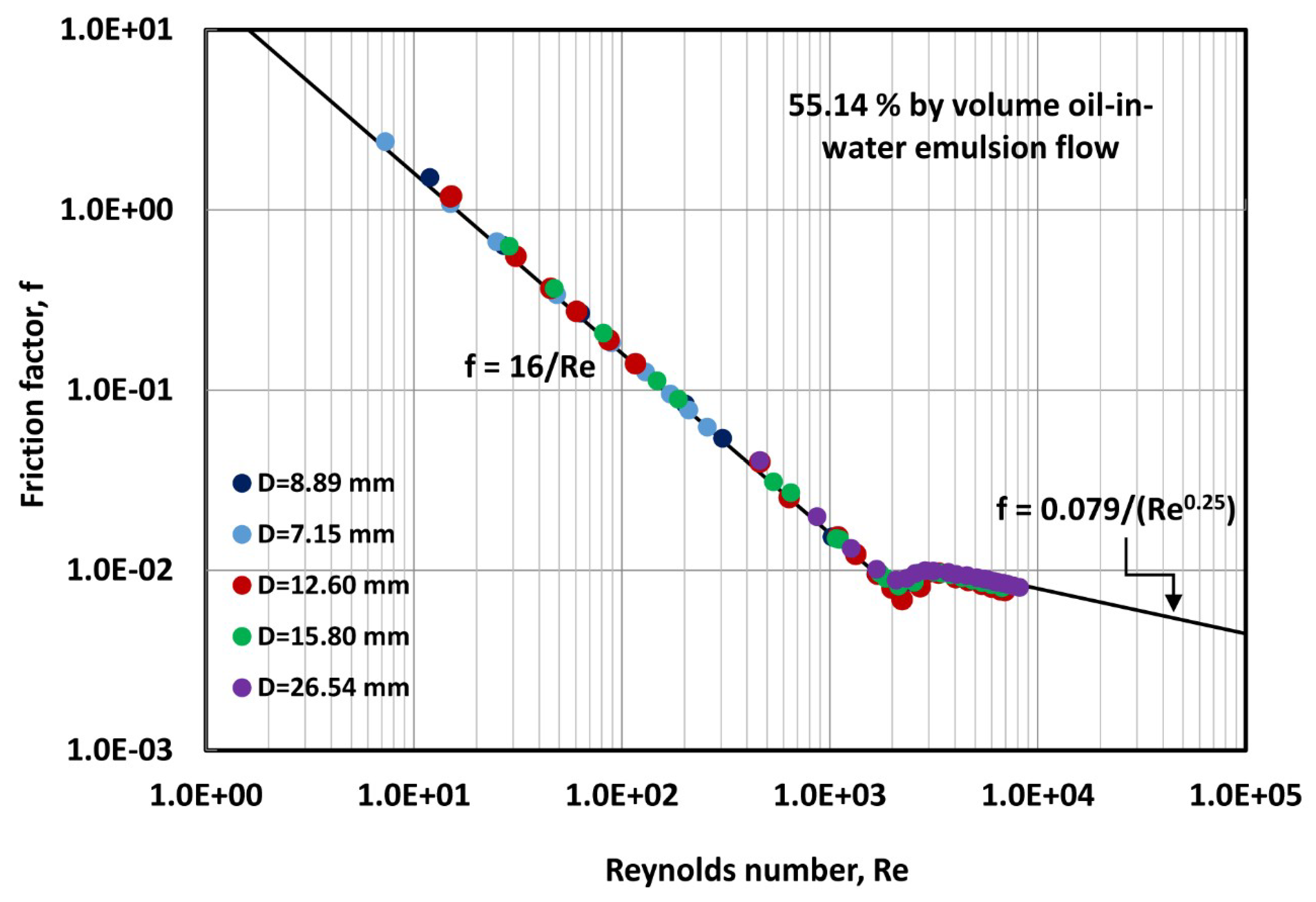
The data are plotted on a log-log scale and compared with the predictions of available theoretical and empirical relations (Equation (40) for laminar flow and Equation (43) for turbulent flow in hydraulically smooth pipes).
4.2. Entropy Generation Results
The entropy generation rate in pipeline flow is calculated from pressure drop versus flow rate measurements using Equation (52), re-written as:
where .
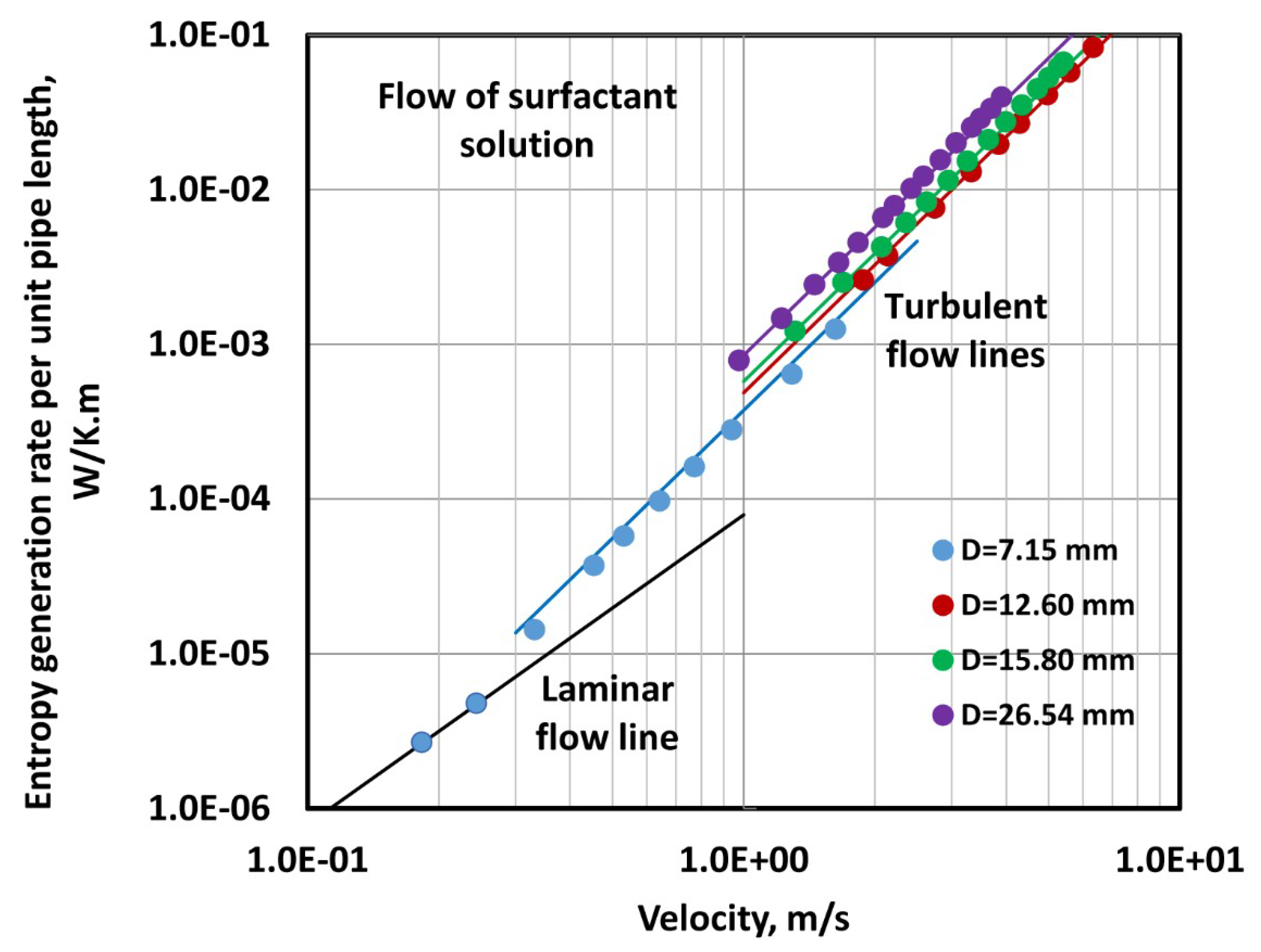
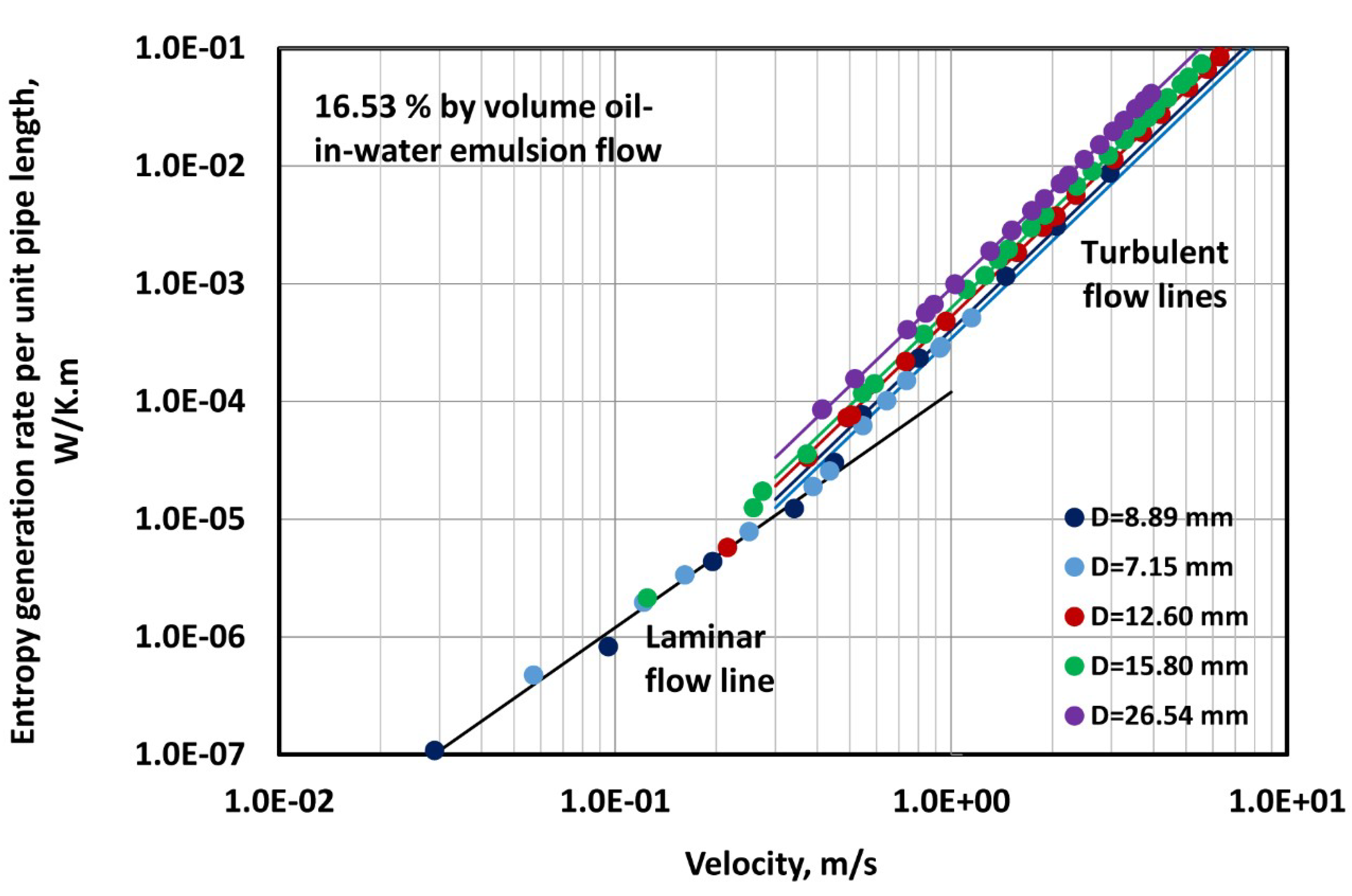
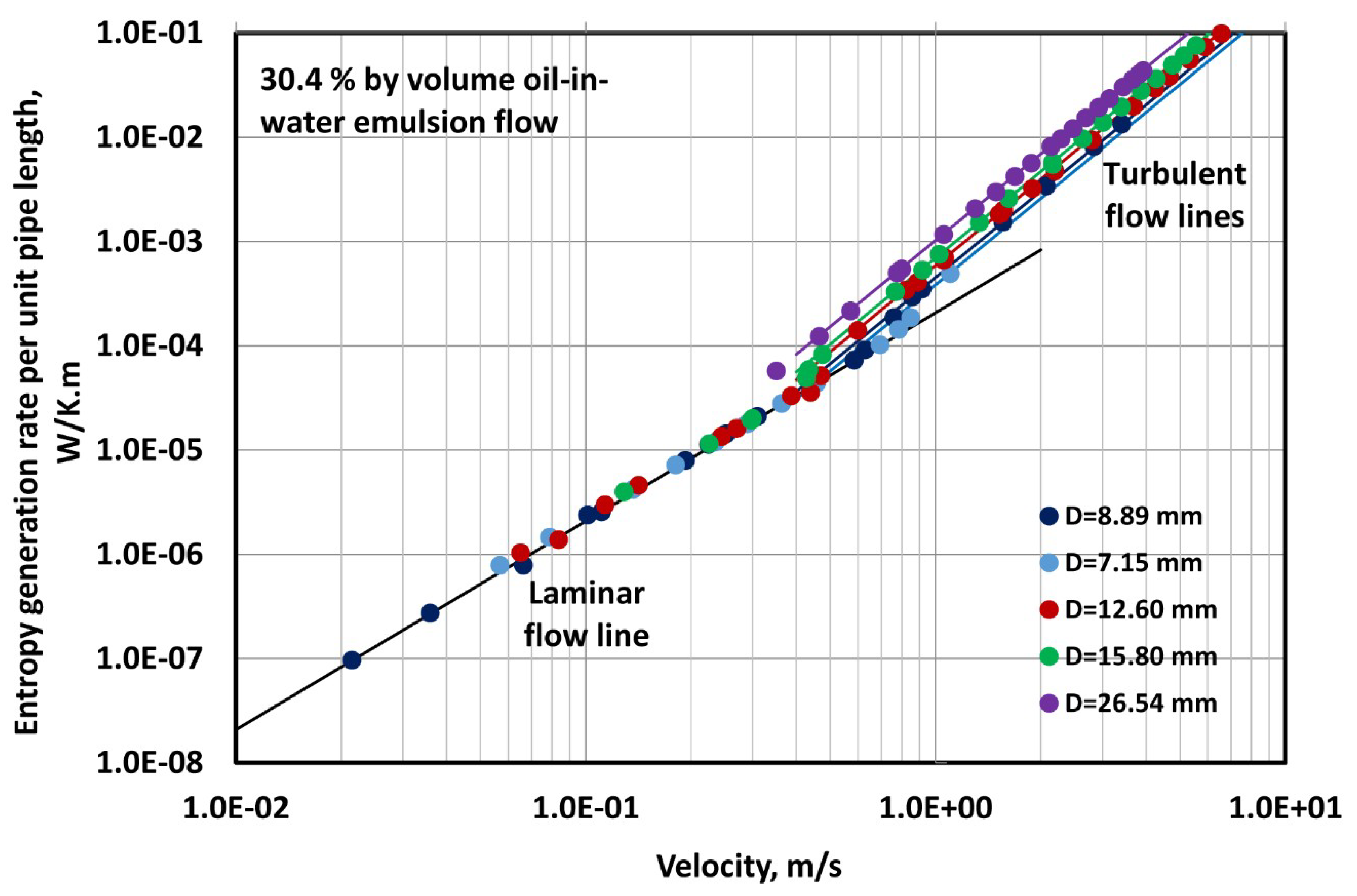
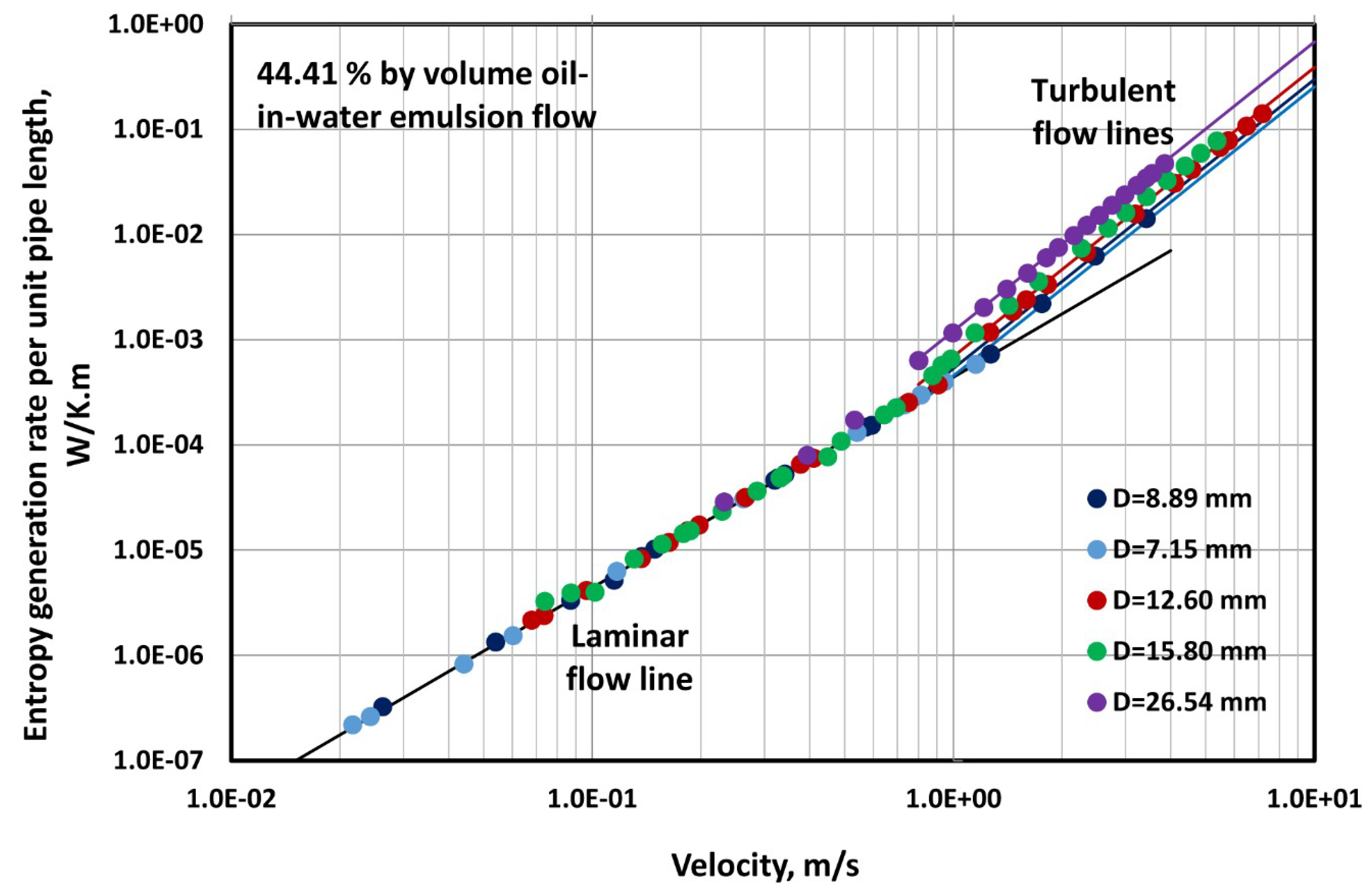
The data are plotted on a log-log scale and compared with the predictions of equations developed in Section 2.4, that is, Equation (54) for laminar flows and Equation (55) for turbulent flows in smooth pipes.
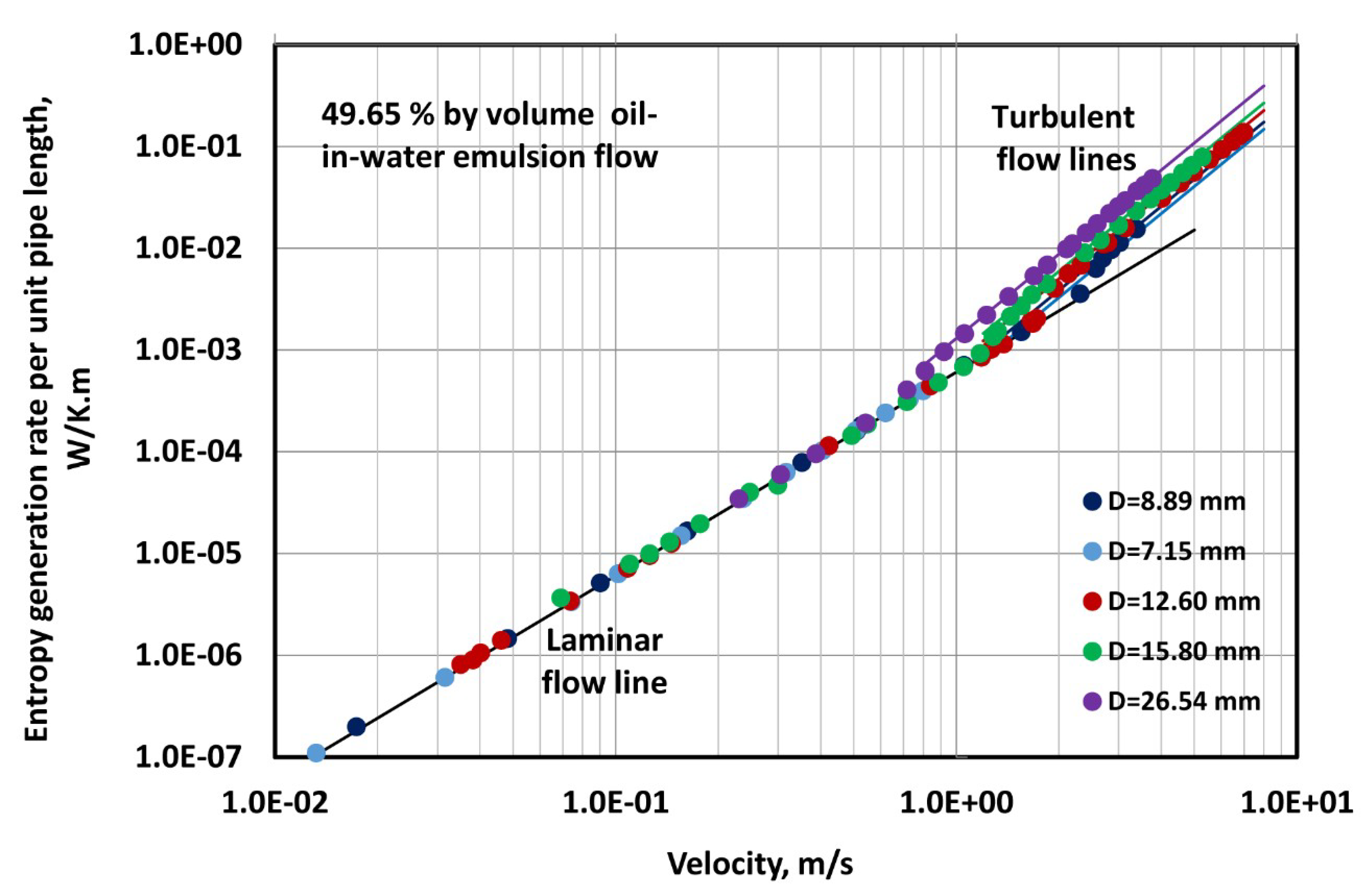
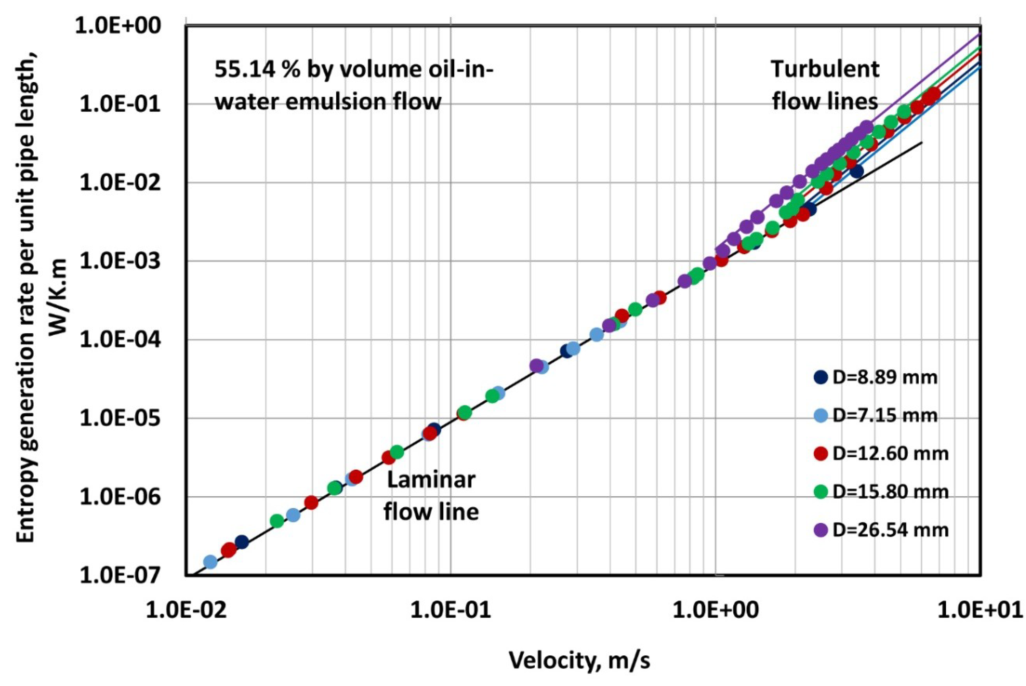
Figure 9, Figure 10, Figure 11, Figure 12, Figure 13 and Figure 14 show the data for different test fluids obtained from different diameter pipelines. As expected from Equation (54), the experimental data corresponding to laminar flow is independent of the pipe diameter. Also, the slope of the laminar flow line is 2 as predicted by Equation (54). Equation (54) describes the laminar flow data adequately for all the test fluids investigated. According to Equation (55), the turbulent flow data for a given diameter pipeline should follow a straight line on a log-log scale with a slope of 2.75. As expected, the experimental data in turbulent regime follow a straight line of slope 2.75. With the increase in pipe diameter, the entropy generation rate increases. The line shifts upward with the increase in pipe diameter but the slope remains the same, that is, 2.75. Thus Equation (55) describes entropy generation in turbulent flows reasonably well.
4.3. Mechanism of Entropy Generation in Real Flows
In real flows, entropy generation is a volumetric phenomenon caused by friction (non-zero viscosity) in fluids. Due to non-zero viscosity of real fluids, velocity gradients and viscous stresses are set up when fluid is forced to flow through a pipe. The presence of viscous stresses and velocity gradients in the fluid cause mechanical energy dissipation into frictional heating effect (internal energy). The degradation of highly ordered mechanical energy into disorderly internal energy results in entropy generation.
The entropy generation rate per unit volume of fluid in real flows (can be expressed as [13]:
where is the viscous stress tensor and is the velocity gradient tensor. It should be noted that we are assuming that there are no temperature gradients in the fluid. If temperature is not uniform and temperature gradients are present, then entropy generation can occur due to another mechanism, namely, irreversible transfer of heat.
In general, the local entropy generation rate per unit volume of fluid ( will vary with the position coordinates. As an example, we illustrate the application of Equation (60) to steady laminar flow in cylindrical pipes. For steady laminar flow of a fluid in a uniform diameter pipe, the term simplifies to:
From Equations (60) and (61), it follows that:
From Newton’s law of viscosity,
Consequently,
The velocity distribution in steady laminar flow of a Newtonian fluid is given as:
Thus,
From Equations (64) and (66), we get:
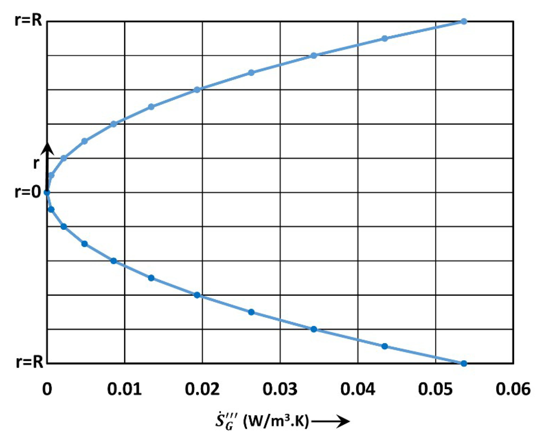
This equation describes the local rate of entropy generation per unit volume in steady laminar flow of a Newtonian fluid in cylindrical pipe of uniform diameter. Figure 15 shows the plot of as a function of radial position. The plot is generated using Equation (67). is zero at the centre of the pipe as velocity gradiant and hence local dissipation of mechanical energy into frictional heating is zero at the centre of the pipe. As we go towards the pipe wall, the local entropy generation increases due to an increase in the velocity gradient and hence frictional heating of the fluid.
Finally it can be readily shown that the global rate of entropy generation (Equation (54)) follows from the integration of the local rate of entropy generation. The global entropy generation rate per unit length can be expressed as:
From Equations (67) and (68), we get:
This is the same result that was obtained earlier in Equation (54).
5. Conclusions
In conclusion, a novel approach is described to teach the second law of thermodynamics with the help of an undergraduate fluid mechanics laboratory involving pipeline flow experiments. The relevant background in fluid mechanics and thermodynamics is reviewed briefly. The link between entropy generation and pressure loss in pipeline flow experiments is demonstrated both theoretically and experimentally. Experimental work involving flow of emulsion-type test fluids in different diameter pipes is carried out to determine friction factor versus Reynolds number behavior and entropy generation rates in pipeline flows. Entropy generation in pipeline flows is explained mechanistically considering local entropy generation in the presence of viscous stresses and velocity gradients in flow of real fluids.
Funding
This research received no external funding.
Conflicts of Interest
The author declares no conflict of interest.
References
- Welty, J.R.; Wicks, C.E.; Wilson, R.E.; Rorrer, G. Fundamentals of Momentum, Heat, and Mass Transfer, 4th ed.; Wiley: New York, NY, USA, 2001. [Google Scholar]
- Greenkorn, R.A.; Kessler, D.P. Transfer Operations; McGraw-Hill: New York, NY, USA, 1972. [Google Scholar]
- Smith, J.M.; Van Ness, H.C.; Abbott, M.M. Introduction to Chemical Engineering Thermodynamics, 7th ed.; McGraw-Hill: New York, NY, USA, 2005. [Google Scholar]
- Bird, R.B.; Stewart, W.E.; Lightfoot, E.N. Transport Phenomena, 2nd ed.; Wiley: New York, NY, USA, 2007. [Google Scholar]
- Colebrook, C.F. Turbulent flow in pipes with particular reference to the transition region between smooth and rough pipe laws. J. Inst. Civ. Eng. 1939, 11, 133–156. [Google Scholar] [CrossRef]
- Colebrook, C.F.; White, C.M. Experiments with fluid friction in roughened pipes. Proc. R. Soc. Lond. Ser. A. Maths. Phys. Sci. 1937, 161, 367–381. [Google Scholar]
- Asker, M.; Turgut, O.E.; Coban, M.T. A review of non iterative friction factor correlations for the calculation of pressure drop in pipes. Bitlis Eren Univ. J. Sci. Technol. 2014, 4, 1–8. [Google Scholar]
- Brkic, D. Review of explicit approximations to the Colebrook relation for flow friction. J. Pet. Sci. Eng. 2011, 77, 34–48. [Google Scholar] [CrossRef] [Green Version]
- Fang, X.; Xu, Y.; Zhou, Z. New correlations of single-phase friction factor for turbulent pipe flow and evaluation of existing single-phase friction factor correlations. Nuclear Eng. Des. 2011, 241, 897–902. [Google Scholar] [CrossRef]
- Zigrang, D.J.; Sylvester, N.D. Explicit approximations to the solution of Colebrook’s friction factor equation. AIChE J. 1982, 28, 514–515. [Google Scholar] [CrossRef]
- Pal, R. Entropy production in pipeline flow of dispersions of water in oil. Entropy 2014, 16, 4648–4661. [Google Scholar] [CrossRef]
- Pal, R. Second law analysis of adiabatic and non-adiabatic pipeline flows of unstable and surfactant-stabilized emulsions. Entropy 2016, 18, 113. [Google Scholar] [CrossRef]
- Pal, R. Entropy generation and exergy destruction in flow of multiphase dispersions of droplets and particles in a polymeric liquid. Fluids 2018, 3, 19. [Google Scholar] [CrossRef]
Figure 1.
Stresses acting on fluid inside the control volume.

Figure 2.
Entropy generation rate per unit length of pipe as a function of average velocity in the pipe.
Figure 2.
Entropy generation rate per unit length of pipe as a function of average velocity in the pipe.

Figure 3.
Friction factor versus Reynolds number data for aqueous surfactant solution.

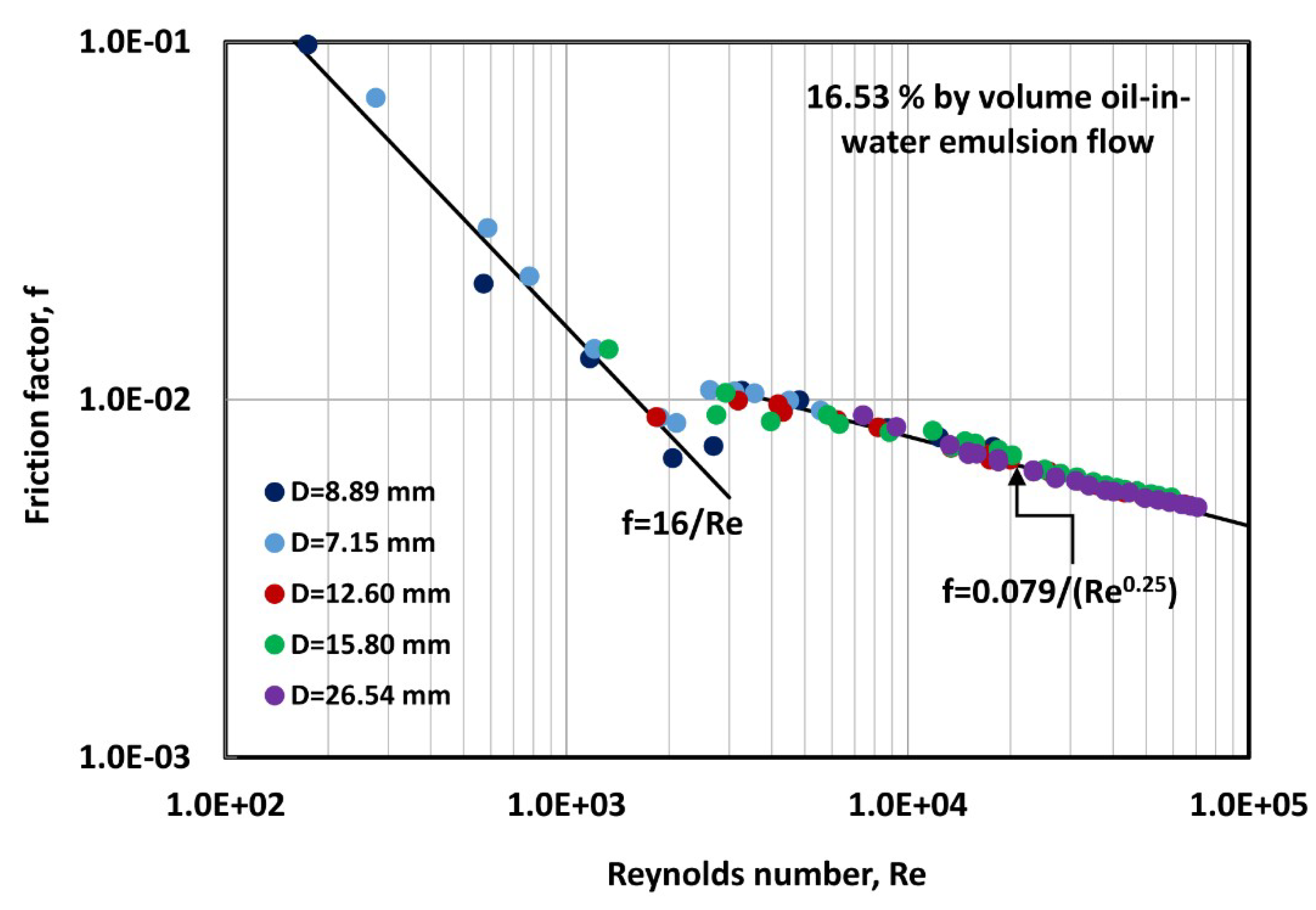
Figure 4.
Friction factor versus Reynolds number data for 16.53% by volume oil-in-water emulsion.

Figure 5.
Friction factor versus Reynolds number data for 30.4% by volume oil-in-water emulsion.

Figure 6.
Friction factor versus Reynolds number data for 44.41% by volume oil-in-water emulsion.

Figure 7.
Friction factor versus Reynolds number data for 49.65% by volume oil-in-water emulsion.

Figure 8.
Friction factor versus Reynolds number data for 55.14% by volume oil-in-water emulsion.

Figure 9.
Entropy generation rate per unit length of pipe as a function of average velocity in flow of aqueous surfactant solution.
Figure 9.
Entropy generation rate per unit length of pipe as a function of average velocity in flow of aqueous surfactant solution.

Figure 10.
Entropy generation rate per unit length of pipe as a function of average velocity in flow of 16.53% by volume oil-in-water emulsion.
Figure 10.
Entropy generation rate per unit length of pipe as a function of average velocity in flow of 16.53% by volume oil-in-water emulsion.

Figure 11.
Entropy generation rate per unit length of pipe as a function of average velocity in flow of 30.4% by volume oil-in-water emulsion.
Figure 11.
Entropy generation rate per unit length of pipe as a function of average velocity in flow of 30.4% by volume oil-in-water emulsion.

Figure 12.
Entropy generation rate per unit length of pipe as a function of average velocity in flow of 44.41% by volume oil-in-water emulsion.
Figure 12.
Entropy generation rate per unit length of pipe as a function of average velocity in flow of 44.41% by volume oil-in-water emulsion.

Figure 13.
Entropy generation rate per unit length of pipe as a function of average velocity in flow of 49.65% by volume oil-in-water emulsion.
Figure 13.
Entropy generation rate per unit length of pipe as a function of average velocity in flow of 49.65% by volume oil-in-water emulsion.

Figure 14.
Entropy generation rate per unit length of pipe as a function of average velocity in flow of 55.14% by volume oil-in-water emulsion.
Figure 14.
Entropy generation rate per unit length of pipe as a function of average velocity in flow of 55.14% by volume oil-in-water emulsion.

Figure 15.
Local entropy generation rate per unit volume () as a function of radial position in laminar flow of a Newtonian fluid (R = 10 mm, T = 298.15 K, µ = 10 mPa·s, ).
Figure 15.
Local entropy generation rate per unit volume () as a function of radial position in laminar flow of a Newtonian fluid (R = 10 mm, T = 298.15 K, µ = 10 mPa·s, ).


Table 1.
Various dimensions of the pipeline flow test sections.
| Pipe Inside Diameter (mm) | Entrance Length (m) | Length of Test Section (m) | Exit Length (m) |
|---|---|---|---|
| 7.15 | 1.07 | 3.05 | 0.46 |
| 8.89 | 0.89 | 3.35 | 0.48 |
| 12.60 | 1.19 | 2.74 | 0.53 |
| 15.8 | 1.65 | 2.59 | 0.56 |
| 26.54 | 3.05 | 1.22 | 0.67 |
Table 2.
Viscosity and density of test fluids.
| Test Fluid Type | Viscosity, mPa·s | Density, kg/m3 |
|---|---|---|
| Aqueous surfactant solution | 0.935 | 997.5 |
| 16.53% O/W emulsion | 1.424 | 961.56 |
| 30.4% O/W emulsion | 2.464 | 931.38 |
| 44.4% O/W emulsion | 5.216 | 900.90 |
| 49.65% O/W emulsion | 7.159 | 889.51 |
| 55.14% O/W emulsion | 10.628 | 877.56 |
© 2019 by the author. Licensee MDPI, Basel, Switzerland. This article is an open access article distributed under the terms and conditions of the Creative Commons Attribution (CC BY) license (http://creativecommons.org/licenses/by/4.0/).
Share and Cite
MDPI and ACS Style
Pal, R. Teaching Fluid Mechanics and Thermodynamics Simultaneously through Pipeline Flow Experiments. Fluids 2019, 4, 103. https://0-doi-org.brum.beds.ac.uk/10.3390/fluids4020103
AMA Style
Pal R. Teaching Fluid Mechanics and Thermodynamics Simultaneously through Pipeline Flow Experiments. Fluids. 2019; 4(2):103. https://0-doi-org.brum.beds.ac.uk/10.3390/fluids4020103
Chicago/Turabian StylePal, Rajinder. 2019. "Teaching Fluid Mechanics and Thermodynamics Simultaneously through Pipeline Flow Experiments" Fluids 4, no. 2: 103. https://0-doi-org.brum.beds.ac.uk/10.3390/fluids4020103