Reynolds Stress Perturbation for Epistemic Uncertainty Quantification of RANS Models Implemented in OpenFOAM


1
Department of Engineering, Aarhus University, 8000 Aarhus C, Denmark
2
Kamstrup A/S, Industrivej 28, Stilling, 8660 Skanderborg, Denmark
*
Authors to whom correspondence should be addressed.
†
Current address: SGL Carbon GmbH, Werner-von-Siemens-Strasse 18, 86405 Meitingen, Germany.
Fluids 2019, 4(2), 113; https://0-doi-org.brum.beds.ac.uk/10.3390/fluids4020113
Submission received: 3 May 2019
/
Revised: 16 June 2019
/
Accepted: 18 June 2019
/
Published: 22 June 2019
(This article belongs to the Special Issue Recent Numerical Advances in Fluid Mechanics)
Abstract
:Reynolds-averaged Navier-Stokes (RANS) models are widely used for the simulation of engineering problems. The turbulent-viscosity hypothesis is a central assumption to achieve closures in this class of models. This assumption introduces structural or so-called epistemic uncertainty. Estimating that epistemic uncertainty is a promising approach towards improving the reliability of RANS simulations. In this study, we adopt a methodology to estimate the epistemic uncertainty by perturbing the Reynolds stress tensor. We focus on the perturbation of the turbulent kinetic energy and the eigenvalues separately. We first implement this methodology in the open source package OpenFOAM. Then, we apply this framework to the backward-facing step benchmark case and compare the results with the unperturbed RANS model, available direct numerical simulation data and available experimental data. It is shown that the perturbation of both parameters successfully estimate the region bounding the most accurate results.
1. Introduction
The motion of a fluid in the turbulent regime is fully described by the Navier-Stokes equations. A numerical solution encompassing all spatial and temporal scales is referred to as direct numerical simulation (DNS). Due to the significant computational cost of DNS, approximations like large-eddy simulation (LES) and Reynolds-averaged Navier-Stokes (RANS) have been developed and are more widely used, in particular for practical engineering problems. RANS models use ensemble averages of the physical quantities, thereby decreasing the computational cost of the simulations. Due to the assumptions that are required to achieve closure, all RANS closures naturally introduce structural, or epistemic, uncertainty.
A systematic approach of the epistemic uncertainty quantification (EUQ) in RANS models, focusing on the Reynolds stress tensor, was first proposed by Emory et al. [1]. They introduced perturbation on the Reynolds stress tensor using the barycentric map proposed by Banerjee et al. [2], as a mean to visualize the degree of anisotropy. The same method was used later in a simulation by Gorle et al. [3] comparing RANS with LES results for an under-expanded jet in a supersonic cross flow. Another contribution, proposed by Gorle et al. [3] and further developed by Gorle and Iaccarino [4], was to introduce the perturbation not only in the momentum equations but also in the turbulent scalar fluxes in the scalar transport equation.
Gorle et al. [5] further developed the methodology with the goal of defining the uncertainty in the separation region. They introduced the idea of a marker, which identifies the regions of the flow where the introduction of perturbations would be useful. In this case the marker is designed to recognize regions with parallel shear flow. Emory et al. [6] recognized the importance of testing the method for various cases and successfully applied EUQ to plane channel flow, square duct flow and a shock/boundary layer interaction with flow separation. In their work, they showed that the method is model-independent.
The latest contribution to EUQ taken into consideration for this research was provided by Iaccarino et al. [7]. In their studies, they proposed a combined perturbation of different quantities in the normalized Reynolds stress tensor. They focused on the simultaneous perturbation of eigenvalues and eigenvectors, which is refered as eigenspace perturbation. With this approach, the ellipsoid describing the eigenspace not only varies in its shape but also in its orientation.
This article is organized as follows. Section 2 presents the mathematical details of the EUQ approach. This methodology is applied to a turbulent flow over a backward-facing step. Section 3 presents the behaviour of the pressure coefficient, friction coefficient, mean velocity field and Reynolds stress tensor after perturbing the eigenvalues and the turbulent kinetic energy separately. These results are compared to the DNS data [8] and the experimental results [9]. A summary and conclusions are provided in Section 4.
2. Methodology
2.1. Epistemic Uncertainty
RANS models decompose the quantities into an averaged part and a fluctuating part such that
Substituting (1) into the Navier–Stokes equations and applying Reynolds averaging leads to the RANS equations (see e.g., [10,11,12])
and the Reynolds-averaged incompressibility constraint
where t is time, is the mean velocity in the direction, where respectively represents the streamwise (x), wall-normal (y) and lateral (z) directions, is the mean kinematic pressure, is the kinematic viscosity, and
is the Reynolds stress tensor. The Reynolds stress tensor is an extra term that arises as a result of the Reynolds decomposition and contains the fluctuating parts of the velocity.
The closure problem in RANS amounts to finding approximations for that do not include the fluctuating part, since that information is not available in an actual RANS simulation. Yet, any model for will be an approximation that introduces an additional epistemic uncertainty. Most popular RANS closure models are based on the Boussinesq turbulent-viscosity hypothesis (or eddy-viscosity hypothesis) that approximates the Reynolds stress tensor as a function of the stretching tensor (mean strain-rate tensor ), the turbulent kinetic energy () and the turbulent viscosity (effect of turbulent eddies on the flow ) such that
2.2. Decomposition of the Reynolds Stress Tensor
The Reynolds stress tensor can be decomposed into components that establish its amplitude, shape and orientation. This is done by defining the turbulence anisotropy tensor as
Equation (6) can be normalized by dividing by , yielding
The eigenvalues of are non-negative due to the condition of realizability established by Speziale et al. [13] and the Cauchy–Schwartz inequality holds for the off-diagonal components. Hence, the values are constrained within the intervals
and
In view of (7), the Reynolds stress tensor can be written as
The eigendecomposition of the normalized anisotropy tensor yields (see e.g., [14])
where
- is a diagonal tensor containing the eigenvalues of the anisotropy tensor in an order such that ,
- is a tensor containing the eigenvectors of the anisotropy tensor in the same order as the eigenvalues.
Isolating in (11) yields
2.3. Perturbation of the Reynolds Stress Tensor
In Section 2.2, the Reynolds stress tensor is rearranged into components that define the amplitude (k), shape () and orientation (v). Perturbation of these components yields an estimate on the epistemic uncertainty. The perturbation yields
where
- is the perturbation on the orientation of the Reynolds stresses,
- is the perturbation on the anisotropy of the Reynolds stresses,
- and , is the amplitude of the perturbation of the turbulent kinetic energy. It is established as a range with a minimum and a maximum .
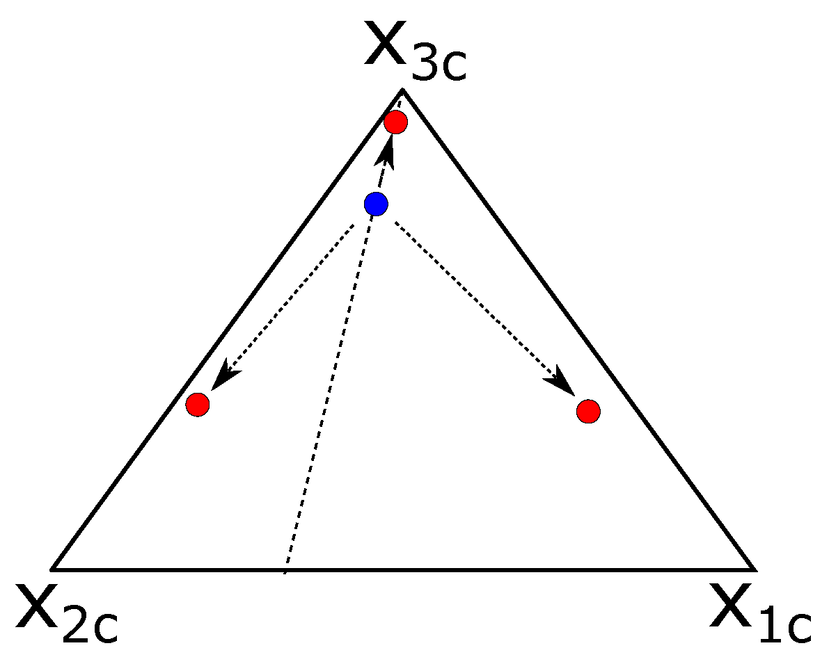
In this article, we focus on the perturbation of the turbulent kinetic energy k and the eigenvalues . The perturbation of k is realized through the parameter that determines the limits of perturbation. The maximum perturbation corresponds to and the minimum to . The perturbation of the eigenvalues is realized using the barycentric map proposed by Banerjee et al. [2] and illustrated in Figure 1.
The barycentric map can represent any stress tensor as a function of the limiting states: one-component, two-component and three-component turbulence. The limiting states
are functions of the eigenvalues associated with the Reynolds stress tensor. The limiting states are normalized such that
The limiting state of the tensor can be represented in a two-dimensional coordinate system with coordinates
or
where = , = and = .
Once the coordinates of the anisotropy tensor are located in the barycentric map, the perturbation is based on two parameters, the direction of the perturbation and the magnitude of perturbation . The direction of the perturbation defines the chosen corner in the barycentric map and magnitude describes the distance of displacement to the chosen corner in the barycentric map in a range of as shown in Figure 1,
The perturbed eigenvalues are calculated as [6]
Here, it is noteworthy to mention that, in the RANS simulation of two-dimensional flows using eddy-viscosity models, at least one of the eigenvalues () of the normalized anisotropy tensor () is zero. Hence, all the points in the flow domain will be located along the line representing the plane shear flow (see Figure 1) [6].
3. Results and Analysis
We applied the previously explained methodology to the backward-facing step at (Re is dependent on the step height h, the inlet velocity and the kinematic viscosity , ), for which DNS [15] and experimental data [9] are available. The backward facing step offers a simple two-dimensional case, similar to the canonical channel flow but adds a certain component of complexity in the physics right after the expansion appears.
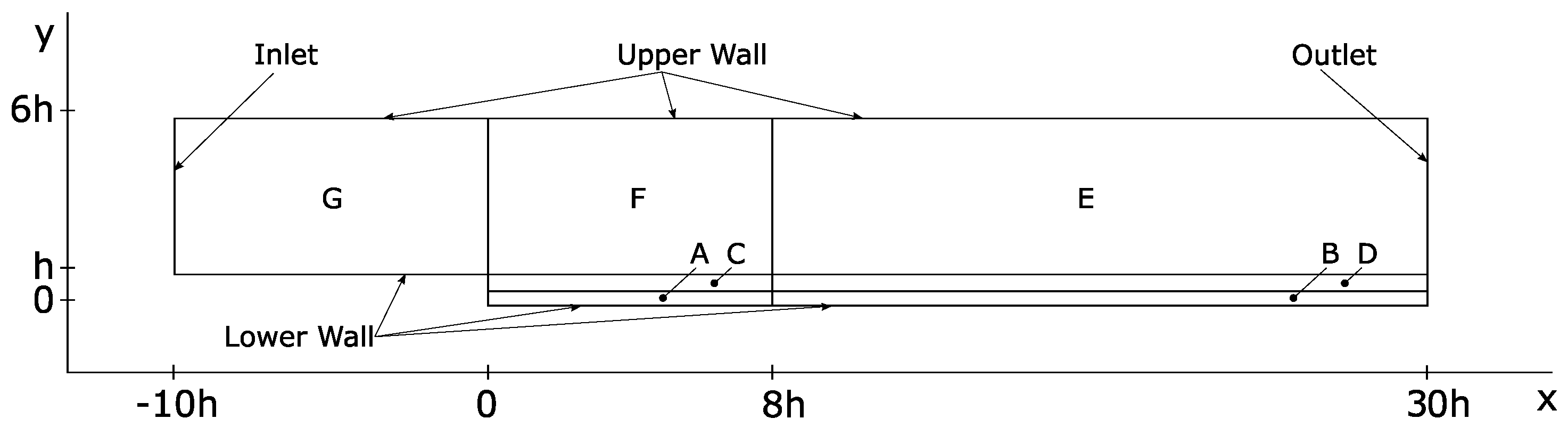
The calculation was performed using the open source software OpenFOAM. The implementation of the Reynolds stress perturbation in OpenFOAM is explained in detail in the Appendix A. The boundary and initial conditions of the case were the same as the ones used by Le and Moin [15] and Jovic and Driver [9], including the mean velocity profile imposed at the inlet by Spalart [16]. They are summarized in Table 1. The k- SST model is chosen as RANS closure. The transport equations and their initial conditions were calculated following Ferziger and Peric [17] and Versteeg and Malalasekera [18]. Figure 2 shows the dimensions of the flow domain and its corresponding areas.
The topology and mesh resolution is similar to the one described in [19]. Three different mesh resolutions were considered to assess the sensitivity of the results to the grid. A relevant parameter to be taken into account, in this case, is the dimensionless wall distance which is defined as
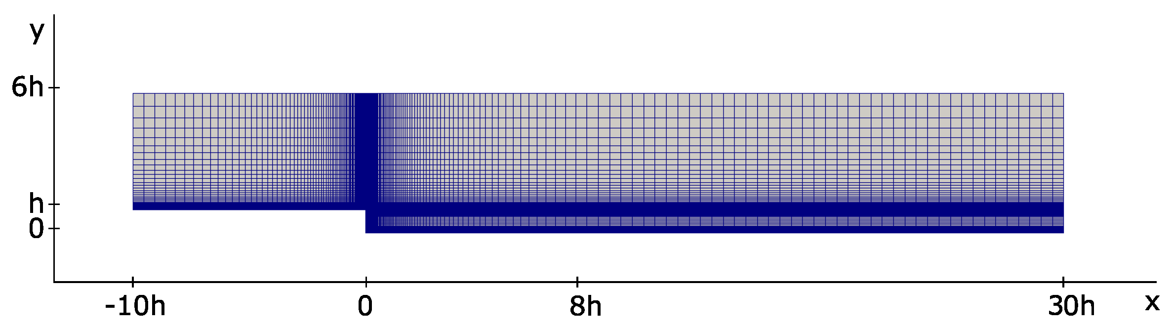
Keeping this value below one () allowed the simulation to capture the physics of the viscous sub-layer. Figure 3 shows the mesh topology. It can be seen that the grid gets finer when it approaches the bottom of the domain and also when it gets closer to the step, which is the most relevant part of the domain. Table 2 summarizes the topology and refinement used in each of the blocks of the domain. The mesh is designed such that the size of the first and last cells can be computed as a function of the grading and the number of cells. The grading is the ratio of the size of the last cell divided by the size of the first cell.
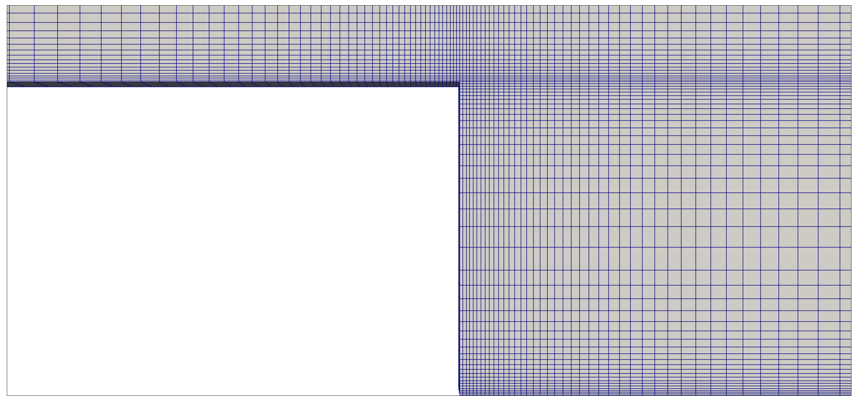
Figure 4 illustrates the zoom into the corner where the step starts and the expansion begins. It can be seen that the size of the cells does not change sharply. It changes smoothly in both directions and it gets finer towards the lower wall.
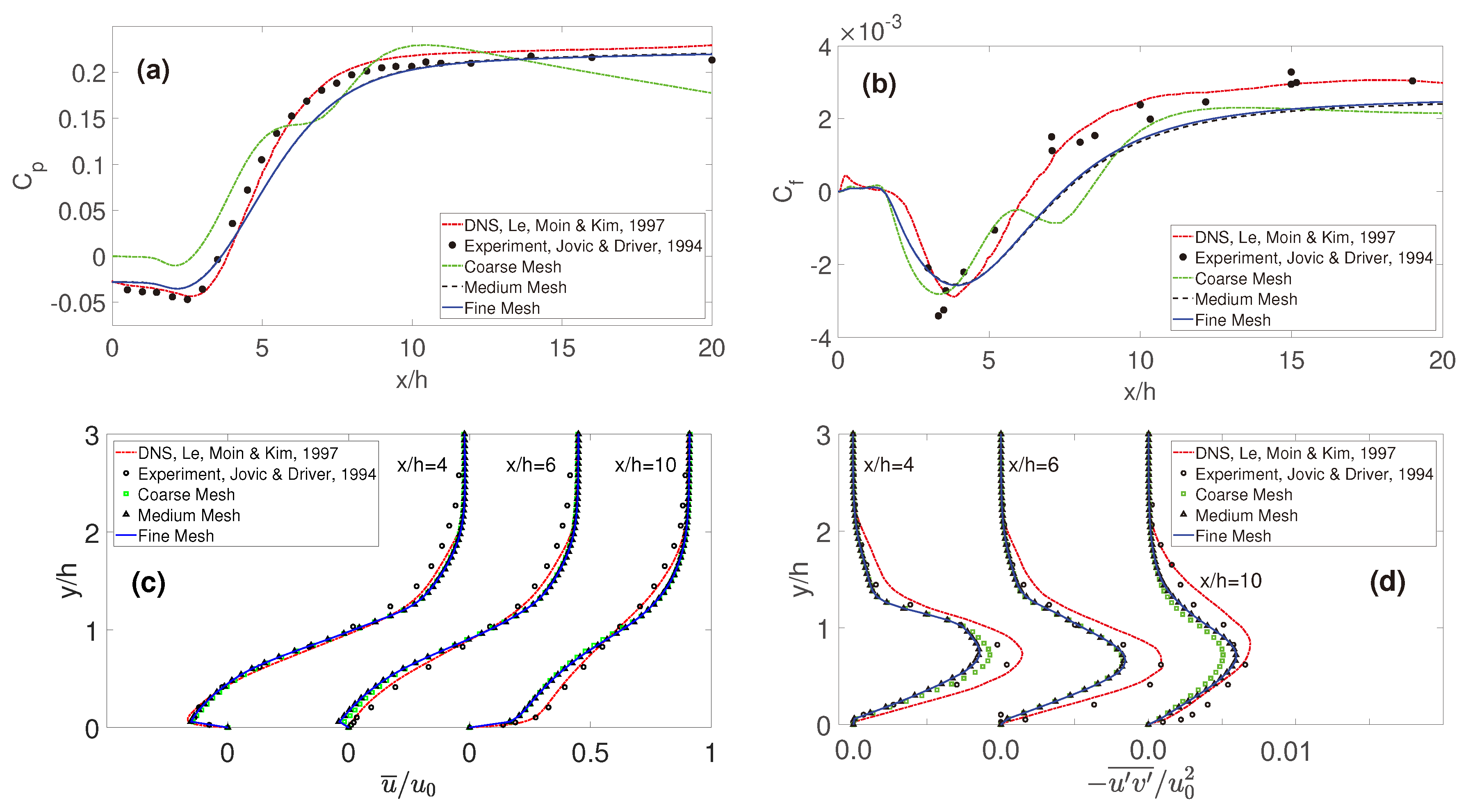
In Figure 5, all three refinements were compared for the pressure coefficient, friction coefficient, mean velocity and Reynolds stresses at , and . The comparisons between different mesh refinements show the grid convergence for the intermediate and the fine grids. The rest of the work is based on the fine mesh described in Table 2. While the focus on the present article are the structural uncertainties in the RANS closures, it is worth mentioning that numerical uncertainties can make up a significant contribution to the overall model error. For a summary of different uncertainty contributions in computational fluid dynamics refer to the ASME standard [20] or more specifically to Roache [21] and Roache [22] in which the estimation of the numerical uncertainty associated with finite grid sizes is addressed.
The following subsections show the behaviour of: pressure coefficient, friction coefficient, mean velocity profile and Reynolds stress computed at several positions in the domain (perturbed and unperturbed). The corresponding DNS and experimental data are also included for comparison.
3.1. Pressure Coefficient
The pressure coefficient was computed at the bottom of the domain throughout the stream-wise direction as
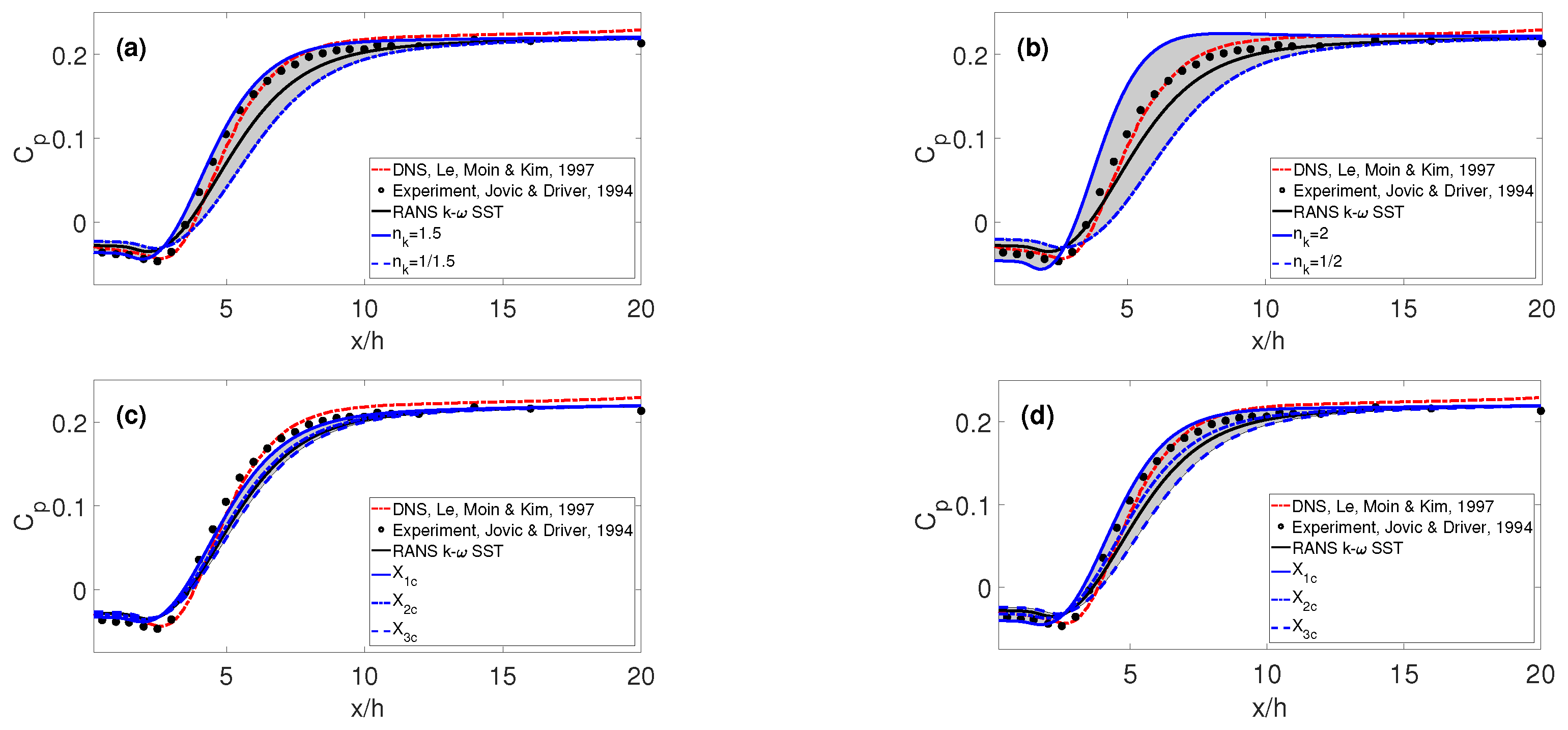
where is the reference wall static pressure, p is the mean pressure computed at any location in the domain and is the upstream freestream reference velocity. We can see in Figure 6 that the results are bounded in a well defined area, thus decreasing the level of uncertainty. We can also see that a small amount of perturbation does not capture properly the physics of the problem. When the amount of perturbation increases, the bounds widen and they are able to cover better the discrepancy between the RANS model and the reference DNS and experimental data.
3.2. Friction Coefficient
The friction coefficient
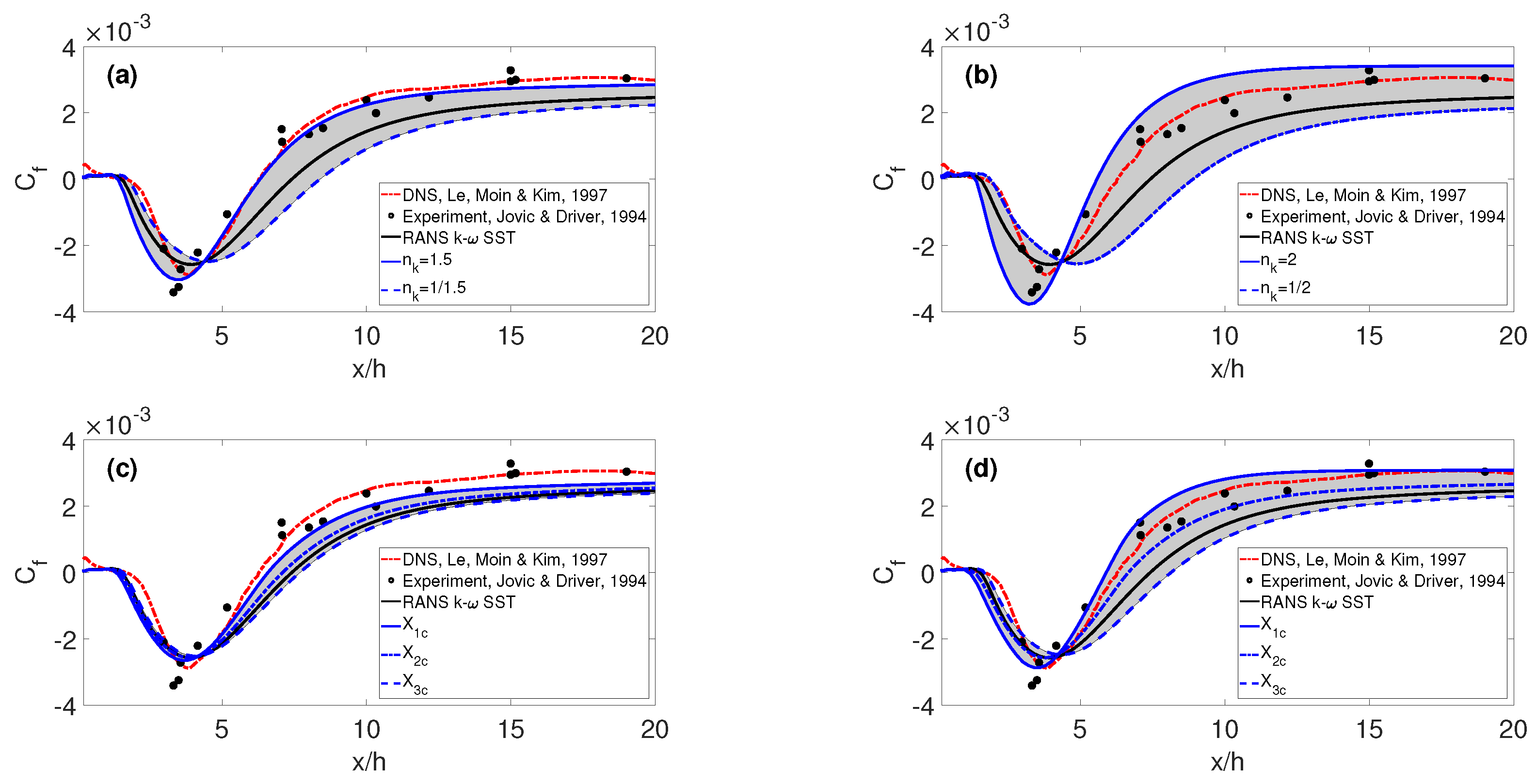
with the wall shear stress was computed at the bottom of the domain, throughout the stream-wise direction. The results seen in Figure 7 show similar behavior as the one seen in Figure 6 with the exception that the turbulent kinetic energy perturbation for almost entirely defines the bounds of discrepancy between RANS and DNS and experimental results.
3.3. Mean Velocity in the x-Direction
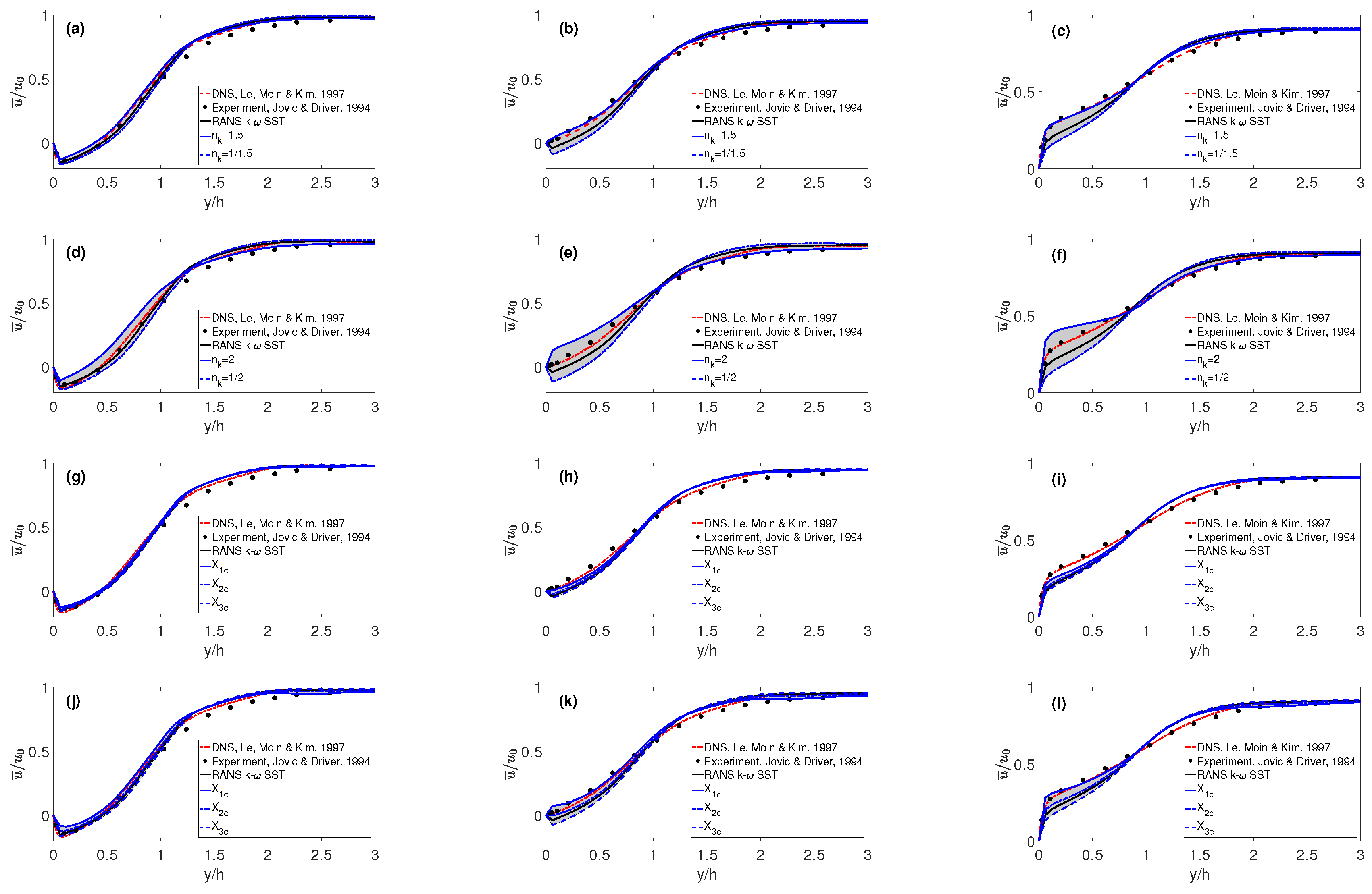
The mean streamwise velocity throughout the y-axis was computed at , and , respectively. The comparison between the models with perturbed kinetic energy, perturbed eigenvalue and the non perturbed model in Figure 8 show the pattern seen in previous parameters. The higher the amount of perturbation, the wider the bounds, thus the proportion of data covered in the bounds is higher. These results show the capability of the framework to capture the uncertainty in the simulation results.
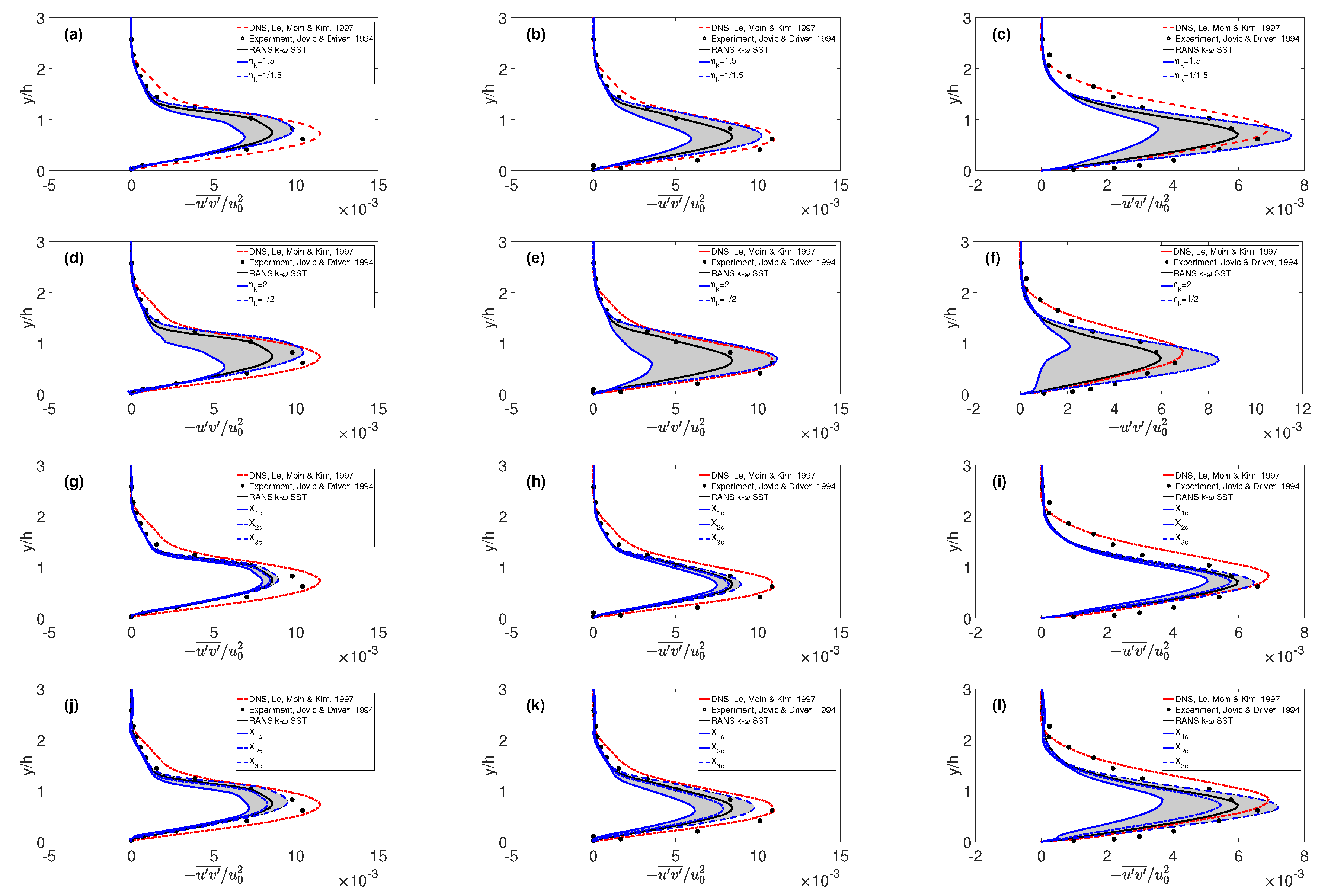
3.4. Reynolds Shear Stress
Reynolds shear stress was computed vertically at , and , respectively, and normalized with respect to the upstream reference velocity. As can be seen from Figure 9, there is some discrepancies between the unperturbed RANS model and the reference data from experiments and DNS. By introducing the structural uncertainties to the RANS, the model can bound the experimental data. It is also observed that the model uncertainty is not uniformly distributed in the domain. In some regions of the flow, the model uncertainty is larger due to the shortcoming of the model assumptions in capturing the physics of the flow. Also, it can be seen that increasing the amount of perturbation in both the magnitude and shape widen the gray regions that envelop the baseline results. For instance, increasing the amount of perturbation for turbulent kinetic energy from to widens the uncertainty bound (gray region) by a factor of about 2. A relatively similar trend is observed when the injected uncertainty into the shape of the stress tensor increases from to .
4. Summary and Conclusions
In this article, we applied the framework, originally proposed by Emory et al. [6] for quantifying the structural uncertainties in RANS models. The quantification consisted in bounding the regions, where the most accurate results are certain to be located. This methodology focuses on the perturbation of the Reynolds stress tensor in the momentum equation. The Reynolds stress tensor is decomposed into components that represent the amplitude (turbulent kinetic energy), the shape (eigenvalues) and the orientation (eigenvectors). This investigation focused only on the influence of the amplitude and shape perturbations.
This perturbation is carried out by the turbulent kinetic energy and the eigenvalues of the Reynolds stress tensor separately and is applied to the backward-facing step case using the open-source software OpenFOAM. In this investigation, the following quantities were monitored: pressure and friction coefficients at the wall, mean streamwise velocity field and the Reynolds stress tensor. The investigation shows promising results. The results showed that for a specific amount of perturbation, the model provides a range of values where the physics of the case are well represented. An interesting feature of this research is that the perturbation of the turbulent kinetic energy shows results as good as the perturbation of the eigenvalues. The eigenvalues have well-established limits of the perturbation through the barycentric map, while the turbulent kinetic energy has not. This implies that the amount of the perturbation applied to the turbulent kinetic energy is not chosen systematically, thus it is left for future investigation.
In view of the results of this article, it is recommended for future work to focus on applying the perturbation to other parameters of the Reynolds stress such as the eigenvectors or a combination that optimizes the range that captures the most precise solution [7]. Recent studies [23,24] suggested that machine learning can be used as a powerful tool to predict discrepancies in the magnitude, anisotropy and orientation of the Reynolds stress tensor. It would be useful to continue applying this methodology to a new set of cases to monitor its behavior.
Author Contributions
Conceptualization, L.F.C.R., D.F.H. and M.A.; methodology, L.F.C.R., D.F.H. and M.A.; software, L.F.C.R.; validation, D.F.H., L.F.C.R. and M.A.; formal analysis, L.F.C.R., D.F.H. and M.A.; investigation, L.F.C.R., D.F.H. and M.A.; resources, D.F.H.; writing—original draft preparation, L.F.C.R.; writing—review and editing, D.F.H. and M.A.; visualization, L.F.C.R.; supervision, D.F.H. and M.A.; project administration, D.F.H. and M.A.
Funding
This research received no external funding.
Acknowledgments
This research was supported by Kamstrup A/S (Group Quality—Fluid Dynamics Center) and Aarhus University. This research is solidly based on the final Master’s Thesis of Luis F. Cremades Rey [25]. The authors also acknowledge the comments by three anonymous reviewers.
Conflicts of Interest
The authors declare no conflict of interest. Kamstrup A/S had no role in the design of the study; in the collection, analyses, or interpretation of data; in the writing of the manuscript, or in the decision to publish the results.
Appendix A. Implementation of the Reynolds Stress Perturbation in OpenFOAM
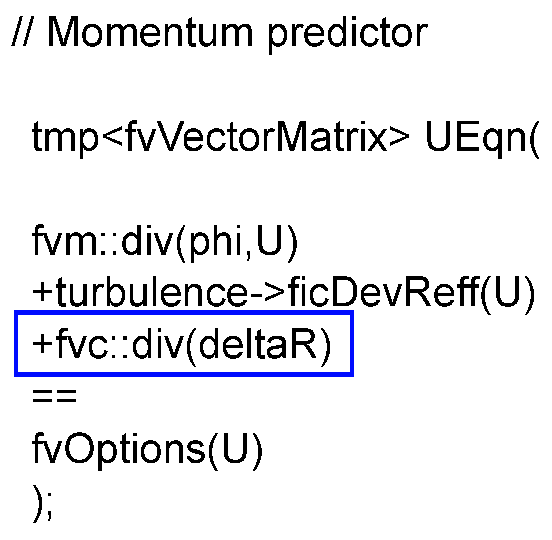
The application of the Reynolds stress perturbation results in the appearance of an extra term (i.e., ) in the right-hand side of Equation (2) as
where is the discrepancy between the perturbed Reynolds stress tensor shown in Equation (14) and the original one. This extra term is evaluated separately and added in OpenFOAM as a new line of code into the momentum equations as highlighted in Figure A1.
Figure A1.
Modification to the Momentum predictor subroutine implemented in OpenFOAM.

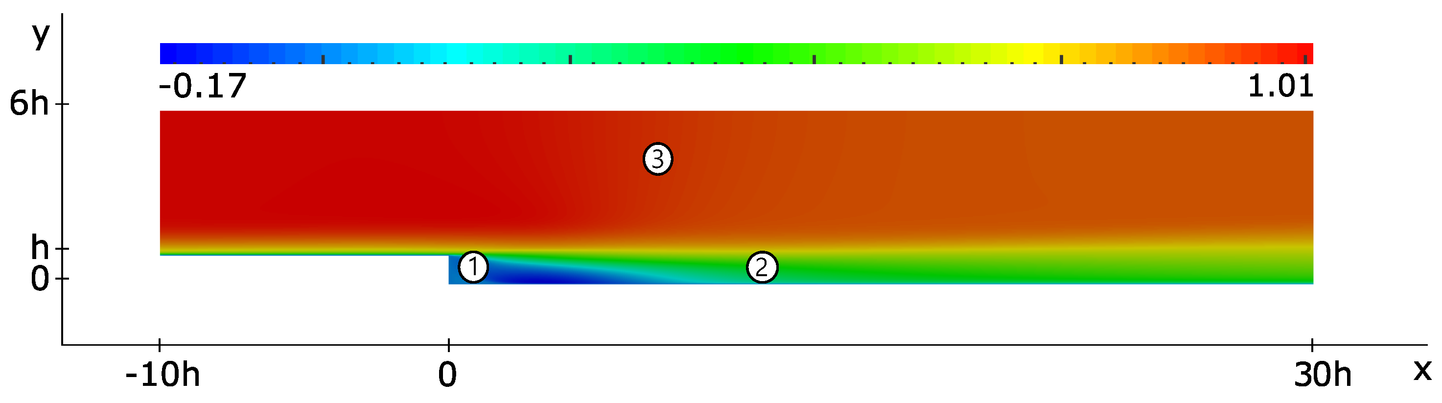
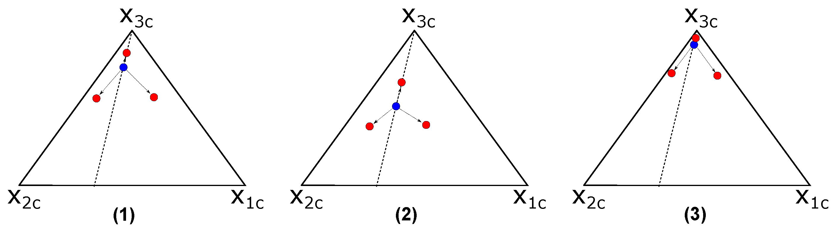
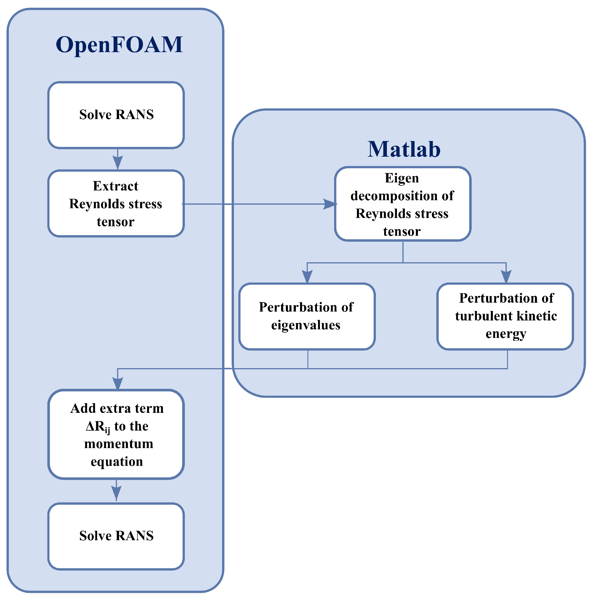
Figure A2 shows the mean velocity field obtained from the baseline RANS solver. To better describe the procedure of the Reynolds stress perturbation, three different locations are chosen and their positions in the barycentric map are shown in Figure A3. This figure shows how the extracted Reynolds stress tensor from the baseline case is perturbed toward different corners in the barycentric map. This procedure is done for all the points in the domain and the perturbed Reynolds stress tensor is computed following Equation (14). Next, the discrepancy between the perturbed Reynolds stress tensor and the original one from the baseline case (i.e., ) is evaluated (here using a separate Matlab code) and added to the right-hand side of the momentum equations in OpenFOAM. The simulations are run again until the results are converged. The corresponding flowchart is also plotted in Figure A4.
Figure A2.
Mean velocity field in the x-direction, normalized with respect to the inlet velocity () obtained from the baseline case. Three different locations have been chosen in the flow domain to study their positions in the barycentric map. The points 1, 2 and 3 are respectively located at (h, ), (, ) and (, ).

Figure A3.
Locations of the chosen points shown in Figure A2 in the barycentric map. The points were perturbed towards the three limiting states and the amount of perturbation is .
Figure A3.
Locations of the chosen points shown in Figure A2 in the barycentric map. The points were perturbed towards the three limiting states and the amount of perturbation is .

Figure A4.
A flowchart describing the implementation of Reynolds stress perturbation in OpenFOAM.

References
- Emory, J.; Pecnik, R.; Iaccarino, G. Modeling Structural Uncertainties in Reynolds-Averaged Computations of Shock/Boundary Layer Interactions. In Proceedings of the AIAA Aerospace Sciences Meeting, Orlando, FL, USA, 4–7 January 2011; p. 0479. [Google Scholar]
- Banerjee, S.; Krahl, R.; Zenger, C.H. Presentation of anisotropy properties of turbulence, invariants versus eigenvalue approaches. J. Fluid Mech. 2007, 8, N32. [Google Scholar] [CrossRef]
- Gorle, C.; Emory, J.; Iaccarino, G. Epistemic uncertainty quantification of RANS modeling for an underexpanded jet in a supersonic cross flow. In Center for Turbulence Research Annual Research Briefs; Center for Turbulence Research, Stanford University: Stanford, CA, USA, 2011; pp. 147–159. [Google Scholar]
- Gorle, C.; Iaccarino, G. A framework for epistemic uncertainty quantification of turbulent scalar flux models for Reynolds-averaged Navier-Stokes simulations. Phys. Fluids 2013, 25, 055105. [Google Scholar] [CrossRef]
- Gorle, C.; Emory, J.; Larsson, J.; Iaccarino, G. Epistemic uncertainty quantification for RANS modeling of the flow over a wavy wall. In Center for Turbulence Research Annual Research Briefs; Center for Turbulence Research, Stanford University: Stanford, CA, USA, 2012; pp. 81–91. [Google Scholar]
- Emory, J.; Larsson, J.; Iaccarino, G. Modeling of structural uncertainties in Reynolds-averaged Navier-Stokes closures. Phys. Fluids 2013, 25, 110822. [Google Scholar] [CrossRef]
- Iaccarino, G.; Mishra, A.A.; Ghili, S. Eigenspace perturbations for uncertainty estimation of single point turbulence closures. Phys. Rev. Fluids 2017, 2, 024605. [Google Scholar] [CrossRef]
- Le, H.; Moin, P.; Kim, J. Direct numerical simulation of turbulent flow over a backward-facing step. J. Fluid Mech. 1997, 330, 349–374. [Google Scholar] [CrossRef] [Green Version]
- Jovic, S.; Driver, D.M. Backward-facing step measurements at low Reynolds number, Reh = 5000. In NASA Technical Memorandum; Technical Report; National Aeronautics and Space Administration (NASA): Washington, DC, USA, 1994; p. 108807. [Google Scholar]
- Patankar, S.V. Numerical Heat Transfer and Fluid Flow, 1st ed.; CRC Press: Boca Raton, FL, USA, 1980. [Google Scholar]
- Pope, S.B. Turbulent Flows, 1st ed.; Cambridge University Press: Cambridge, UK, 2000. [Google Scholar]
- Wilcox, D.C. Turbulence Modeling for CFD, 1st ed.; DCW Industries: La Canada, CA, USA, 1993. [Google Scholar]
- Speziale, C.; Abid, R.; Durbin, P. On the realizability of Reynolds stress turbulence closures. J. Sci. Comput. 1994, 9, 369–403. [Google Scholar] [CrossRef]
- Kreyszig, E. Advanced Engineering Mathematics, 10th ed.; Wiley: Hoboken, NJ, USA, 2001. [Google Scholar]
- Le, H.; Moin, P. Direct numerical simulation of turbulent flow over a backward-facing’ step. In Center for Turbulence Research Annual Research Briefs; Center for Turbulence Research, Stanford University: Stanford, CA, USA, 1992; pp. 161–173. [Google Scholar]
- Spalart, P.R. Direct simulation of a turbulent boundary layer up to ReΘ = 1410. In NASA Technical Memorandum; National Aeronautics and Space Administration (NASA): Washington, DC, USA, 1986; p. 89407. [Google Scholar]
- Ferziger, J.H.; Peric, M. Computational Methods for Fluid Dynamics, 3rd ed.; Springer: Berlin/Heidelberg, Germany, 2001. [Google Scholar]
- Versteeg, H.K.; Malalasekera, W. An Introduction to Computational Fluid Dynamics: The Finite Volume Method, 2nd ed.; Pearson Prentice Hall: Upper Saddle River, NJ, USA, 2007. [Google Scholar]
- Rumsey, C. Turbulence Modeling Resource. Available online: https://turbmodels.larc.nasa.gov (accessed on 3 May 2019).
- The American Society of Mechanical Engineers (ASME). Standard for Verification and Validation in Computational Fluid Dynamics and Heat Transfer; ASME: New York, NY, USA, 2009. [Google Scholar]
- Roache, P.J. Perspective: A method for uniform reporting of grid refinement studies. J. Fluids Eng. 1994, 116, 405–413. [Google Scholar] [CrossRef]
- Roache, P.J. Quantification of uncertainty in computational fluid dynamics. Annu. Rev. Fluid Mech. 1997, 29, 123–160. [Google Scholar] [CrossRef]
- Wu, J.L.; Xiao, H.; Paterson, E. Physics-informed machine learning approach for augmenting turbulence models: A comprehensive framework. Phys. Rev. Fluids 2018, 3, 074602. [Google Scholar] [CrossRef] [Green Version]
- Duraisamy, K.; Iaccarino, G.; Xiao, H. Turbulence modeling in the age of data. Annu. Rev. Fluid Mech. 2019, 51, 357–377. [Google Scholar] [CrossRef]
- Cremades Rey, L.F. Epistemic Uncertainty Quantification of RANS Models. Master’s Thesis, Aarhus University, Aarhus, Denmark, 2018. [Google Scholar]
Figure 1.
Barycentric map. The limiting states are represented in the vertices as one-component , two-component and three-component (isotropic) turbulence. The anisotropy is zero at and maximum at . The dashed line denotes plane shear flow, where at least one of the eigenvalues is zero. The arrows show perturbations toward limiting states of turbulence [6].

Figure 2.
Dimensions of the flow domain as a function of the step height h. The domain is divided in seven blocks in order to design and optimize the mesh. It also shows the location of the boundaries.
Figure 2.
Dimensions of the flow domain as a function of the step height h. The domain is divided in seven blocks in order to design and optimize the mesh. It also shows the location of the boundaries.

Figure 3.
Mesh topology in the flow domain.

Figure 4.
Mesh topology in the flow domain zoomed in where the step is located and expansion starts, .
Figure 4.
Mesh topology in the flow domain zoomed in where the step is located and expansion starts, .

Figure 5.
(a) Convergence of the pressure coefficients calculated at the bottom of the flow domain after and before the expansion, computed as . (b) Convergence of the friction coefficients calculated at the bottom of the flow domain after and before the expansion, computed as . (c) Convergence of the mean streamwise velocity profiles calculated at , , and normalized with respect to the inlet mean velocity (). (d) Convergence of the Reynolds shear stress component calculated at , , and normalized with respect to the inlet mean velocity ().

Figure 6.
Pressure coefficients at , computed as: . (a) Turbulent kinetic energy perturbation , (b) turbulent kinetic energy perturbation , (c) eigenvalue perturbation with and (d) eigenvalue perturbation with . , and represent perturbations toward the three corners of the barycentric map. direct numerical simulation (DNS) data [15] (— ·); experiment data [9] (•); Reynolds-averaged Navier-Stokes (RANS) k- SST model (−). The uncertainty bounds are shown with gray areas.

Figure 7.
Friction coefficients at . Computed as: . (a) Turbulent kinetic energy perturbation , (b) turbulent kinetic energy perturbation , (c) eigenvalue perturbation with and (d) eigenvalue perturbation with . , and represent perturbations toward the three corners of the barycentric map. DNS data [15] (— ·); experiment data [9] (•); RANS k- SST model (−). The uncertainty bounds are shown with gray areas.

Figure 8.
Mean streamwise velocity profiles calculated at , and and normalized by the inlet mean velocity (). (a) k perturbation with at , (b) k perturbation with at , (c) k perturbation with at , (d) k perturbation with at , (e) k perturbation with at , (f) k perturbation with at , (g) eigenvalue perturbation with at , (h) eigenvalue perturbation with at , (i) eigenvalue perturbation with at , (j) eigenvalue perturbation with at , (k) eigenvalue perturbation with at and (l) eigenvalue perturbation with at . , and represent perturbations toward the three corners of the barycentric map. DNS data [15] (— ·); experimental data [9] (•); RANS k- SST model (−). The uncertainty bounds are shown with gray areas.

Figure 9.
Reynolds shear stress calculated at , and and normalized by the inlet mean velocity (). (a) k perturbation with at , (b) k perturbation with at , (c) k perturbation with at , (d) k perturbation with at , (e) k perturbation with at , (f) k perturbation with at , (g) eigenvalue perturbation with at , (h) eigenvalue perturbation with at , (i) eigenvalue perturbation with at , (j) eigenvalue perturbation with at , (k) eigenvalue perturbation with at and (l) eigenvalue perturbation with at . , and represent perturbations toward the three corners of the barycentric map. DNS data [15] (— ·); experimental data [9] (•); RANS k- SST model (−). The uncertainty bounds are shown with gray areas.


Table 1.
Description of the boundary conditions imposed in each part of the flow domain.
| Boundary | Velocity | Pressure |
|---|---|---|
| Upper Wall | No-stress wall | Zero gradient |
| Lower Wall | No-slip condition | Zero gradient |
| Inlet | Non-uniform inlet | Zero gradient |
| Outlet | Zero gradient | Uniform, |
Table 2.
Mesh refinement and topology for each of the three types of refinements applied. The Cells columns represent the amount of cells in each block in the x- and y-direction, respectively. The Grading columns represent the refinement in each block in the x- and y-direction, respectively.
Table 2.
Mesh refinement and topology for each of the three types of refinements applied. The Cells columns represent the amount of cells in each block in the x- and y-direction, respectively. The Grading columns represent the refinement in each block in the x- and y-direction, respectively.
| Coarse Mesh | Intermediate Mesh | Fine Mesh | ||||||||||
|---|---|---|---|---|---|---|---|---|---|---|---|---|
| Cells | Grading | Cells | Grading | Cells | Grading | |||||||
| Block | x | y | x | y | x | y | x | y | x | y | x | y |
| A | 40 | 11 | 50 | 11.29 | 80 | 21 | 50 | 10.61 | 160 | 42 | 50 | 10.91 |
| B | 21 | 11 | 1 | 11.29 | 41 | 21 | 1 | 10.61 | 81 | 42 | 1 | 10.91 |
| C | 40 | 11 | 50 | 0.09 | 80 | 21 | 50 | 0.09 | 160 | 42 | 50 | 0.09 |
| D | 21 | 11 | 1 | 0.09 | 41 | 21 | 1 | 0.09 | 81 | 42 | 1 | 0.09 |
| E | 21 | 20 | 1 | 100 | 41 | 40 | 1 | 100 | 81 | 80 | 1 | 100 |
| F | 40 | 20 | 50 | 100 | 80 | 40 | 50 | 100 | 160 | 80 | 50 | 100 |
| G | 40 | 20 | 0.02 | 100 | 80 | 40 | 0.02 | 100 | 160 | 80 | 0.02 | 100 |
© 2019 by the authors. Licensee MDPI, Basel, Switzerland. This article is an open access article distributed under the terms and conditions of the Creative Commons Attribution (CC BY) license (http://creativecommons.org/licenses/by/4.0/).
Share and Cite
MDPI and ACS Style
Cremades Rey, L.F.; Hinz, D.F.; Abkar, M. Reynolds Stress Perturbation for Epistemic Uncertainty Quantification of RANS Models Implemented in OpenFOAM. Fluids 2019, 4, 113. https://0-doi-org.brum.beds.ac.uk/10.3390/fluids4020113
AMA Style
Cremades Rey LF, Hinz DF, Abkar M. Reynolds Stress Perturbation for Epistemic Uncertainty Quantification of RANS Models Implemented in OpenFOAM. Fluids. 2019; 4(2):113. https://0-doi-org.brum.beds.ac.uk/10.3390/fluids4020113
Chicago/Turabian StyleCremades Rey, Luis F., Denis F. Hinz, and Mahdi Abkar. 2019. "Reynolds Stress Perturbation for Epistemic Uncertainty Quantification of RANS Models Implemented in OpenFOAM" Fluids 4, no. 2: 113. https://0-doi-org.brum.beds.ac.uk/10.3390/fluids4020113