Progress in Phenomenological Modeling of Turbulence Damping around a Two-Phase Interface


1
Nuclear Engineering Division, Department of Physics, KTH Royal Institute of Technology, 106 91 Stockholm, Sweden
2
Institute of Heat Engineering, Warsaw University of Technology, 21/25 Nowowiejska Street, 00-665 Warsaw, Poland
*
Author to whom correspondence should be addressed.
Fluids 2019, 4(3), 136; https://0-doi-org.brum.beds.ac.uk/10.3390/fluids4030136
Submission received: 20 June 2019
/
Revised: 13 July 2019
/
Accepted: 16 July 2019
/
Published: 18 July 2019
(This article belongs to the Special Issue Free surface flows)
Abstract
:The presence of a moving interface in two-phase flows challenges the accurate computational fluid dynamics (CFD) modeling, especially when the flow is turbulent. For such flows, single-phase-based turbulence models are usually used for the turbulence modeling together with certain modifications including the turbulence damping around the interface. Due to the insufficient understanding of the damping mechanism, the phenomenological modeling approach is always used. Egorov’s model is the most widely-used turbulence damping model due to its simple formulation and implementation. However, the original Egorov model suffers from the mesh size dependency issue and uses a questionable symmetric treatment for both liquid and gas phases. By introducing more physics, this paper introduces a new length scale for Egorov’s model, making it independent of mesh sizes in the tangential direction of the interface. An asymmetric treatment is also developed, which leads to more physical predictions for both the turbulent kinetic energy and the velocity field.
1. Introduction
Two-phase flows are widely encountered in nuclear, chemical, and petroleum engineering. Due to the insufficient understanding of the basic mechanisms that govern the two-phase flow, the computational fluid dynamics (CFD) modeling of two-phase systems, where moving interfaces exist, is still challenging, even though many approaches, e.g., the volume of fluid (VOF) method [1], the two-fluid model [2], and the level-set method [3], have been proposed. Since a large portion of the two-phase flows in industrial applications are turbulent, turbulence models should be combined with the proposed two-phase models to simulate such turbulent two-phase flows. However, turbulence modeling for two-phase flows is not as mature as that for single-phase flows. As a result, turbulence models that are developed for single-phase flows are usually employed in two-phase flow simulations with few or no modifications.
The immaturity in both interface modeling and turbulence modeling leads to unphysical predictions, for which one well-known issue is that the turbulence behavior near the interface is mispredicted. For instance, according to both experimental studies [4,5] and direct numerical simulations (DNS) [6,7], the gas–liquid interface in stratified flows behaves similarly to a solid wall in single-phase flows. In order to reproduce this wall-like behavior in CFD simulations where turbulence models are used, researchers have made various attempts trying to damp the turbulence around the interface such that the interface could behave more like a wall [8,9,10,11,12]. Even though all these methods are essentially phenomenological models, they are being used and will still be used in the foreseen future. The reason is that, in the absence of mechanistic models for turbulence damping, these phenomenological models are a useful tool that advances two-phase turbulent CFD simulations. Among all these approaches, the method proposed by Egorov [8] is the most used one for the VOF and two-fluid modeling due to its simple formulation and easy implementation, which will be discussed in detail in Section 2.
Egorov’s model was originally developed for gas–liquid stratified flows so that the near-interface velocity profile could be correctly predicted, and it is still being used for this purpose [13]. In addition, the model has been found to be crucial for the accurate prediction of oil film distribution in an aero-engine bearing chamber [14], of wave propagation [15], and of the entrained fraction in annular flows [16]. This not only shows the popularity of Egorov’s model in a broad range of flow conditions, but also justifies the necessity and usefulness of developing such phenomenological models.
Aside from the popularity, Egorov’s model has its own disadvantages due to its phenomenological modeling nature. On the one hand, a proper value should be selected for the model parameter, B, to match the numerical results with the experimental data. However, B is mesh size sensitive, and no universal guideline exits for the selection of B [8,12,16,17]. On the other hand, Egorov’s model employs the same treatment for both gas and liquid phases, which is referred to as the symmetric treatment by Frederix et al. [12]. It has been pointed out by many researchers [10,12,18] that an asymmetric treatment should be introduced to model the different turbulence behaviors on the different sides of the interface.
This paper aims at modifying Egorov’s model by introducing more physics. A new length scale for the interface is firstly introduced to make Egorov’s model less dependent on the value of B. After some in-depth discussions, an asymmetric treatment is proposed for the turbulence damping such that the turbulence behaviors in individual phases could be modeled separately.
2. Egorov’s Model
The model proposed by Egorov [8] is based on the equation in the framework of RANS modeling of turbulence. There are various forms of equations for different turbulence models, but they can be generalized as:
where denotes density, is the production term, is the dissipation term, and is a transformation term that arises due to the blending of the k- model and the k- model. All three terms are quite complicated since they all include additional unknown variables other than . The remaining is the destruction term , which is much simpler in form in comparison with others. The boundary condition for is determined by the asymptotic solution for in the viscous sublayer, which is known as:
where in Equation (2) is a constant in the k- model, is the dynamic viscosity, and y is the wall distance of the cell. B is a factor that makes sure this term is large enough so that the selection of B will not affect the result for the interface between the fluid and a solid wall. In Menter [19], , and in Menter and Esch [20], .
According to , where is the turbulent viscosity and k is the turbulent kinetic energy, a high leads to a lower ; therefore, a larger can be used to damp the turbulence. This idea is the central pillar of the model proposed by Egorov [8]. In order to introduce turbulence damping for the fluid–fluid interface, a source term is added to the equation so that a larger will be calculated for the interfacial region. In analogy with the destruction term in Equation (1) and treatment for the fluid–solid interface in Equation (2), the following form of source term is proposed:
where subscript i denotes the phase, which means that each phase has a source term based on its property. is the interfacial area density, which is zero for the single-phase region and satisfies the following property for the interfacial region:
where n is the coordinate in the direction normal to the interface. The role of is to guarantee that the source term is only activated in the interfacial region, and the most widely-used form is:
is the typical cell size across the interface, and in most cases, is assumed for the purpose of simplification [13,16,17,21]. Therefore, the source term could be simplified as:
It is quite obvious that grid information appears in this source term explicitly, and it should be noted that is also dependent on mesh size [10]. Therefore, B has to be tuned according to the grid size. If the mesh effect on is neglected, a smaller B should be used for a finer mesh such that the same source term could be used.
In the present study, Egorov’s model is used together with the VOF method due to the simple formulation of VOF.
3. Calculation of
According to Egorov [8], is the typical grid cell size across the interface. However, this statement is somehow ambiguous and leaves room for various interpretations of it.
3.1. Existing Methods
The simplest and most straightforward way is using , where V is the volume of an interfacial cell. This treatment could provide a localized length scale with V, which is always available for a given mesh. This method is adopted in the commercial code STAR-CCM+ [17]. Even though Egorov’s model is not officially provided in open-source software like OpenFOAM, it can be easily implemented by the user. In most cases, users use as the length scale [13,16].
An alternative approach is based on another interpretation of that it is regarded as the cell height normal to the interface. This is adopted by commercial code ANSYS FLUENT [21]. According to this interpretation, both the mesh information and phase distribution are necessary for the calculation of . However, the implementation details of this approach are not provided in the documentation.
3.2. A New Length Scale
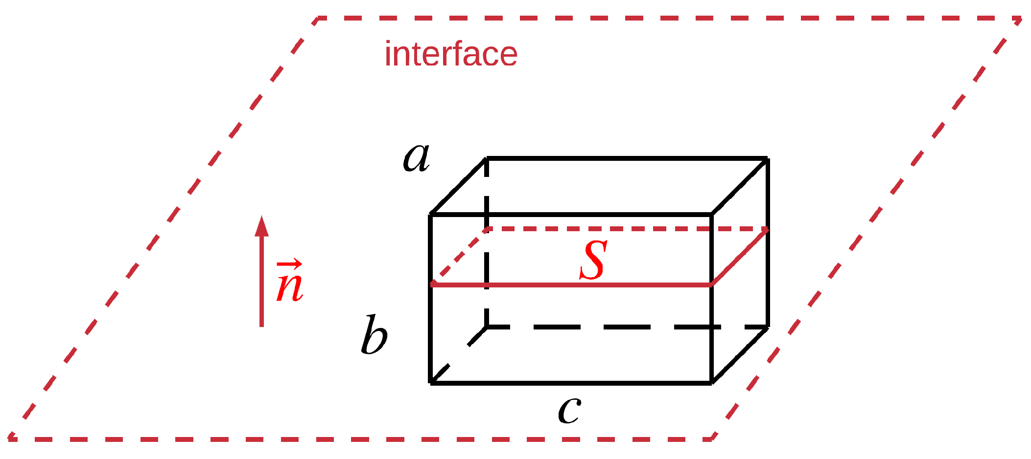
According to the authors’ knowledge, since Equation (3) is proposed based on Equation (2), should be defined in a way that is similar to the definition of y in Equation (2). Then, straightforwardly, could be interpreted as the normal distance between the cell centroid and the interface. This could be done by firstly reconstructing the interface and then measuring the interfacial normal distance for each cell as described by Liovic and Lakehal [9]. However, this is only feasible for VOF methods where the geometric interface reconstruction is applied during the simulation. In addition, could be very tiny or even zero, making the term shown in Equation (6) unbounded. Therefore, this interpretation of is not adopted. In the present study, is calculated based on an approach that does not require the reconstruction of the interface so that it can be applied to more generalized VOF methods. The proposed method was deduced from a simple case as shown in Figure 1.
Assume the interface is perpendicular to four inter-parallel edges of a cuboidal cell. Then, the length of these edges, b, is a good representation for , since it reflects the cell size in the normal direction of the interface. This could also be explained from a mathematical point of view by:
where the numerator is the volume of the cell and the denominator is a characteristic area scale for the interaction between the interface and the cell. It might be interpreted as the area of the interface trimmed by the cell, which is quite intuitive. This common surface of the interface and the cell is denoted by . In Figure 1, we could easily get:
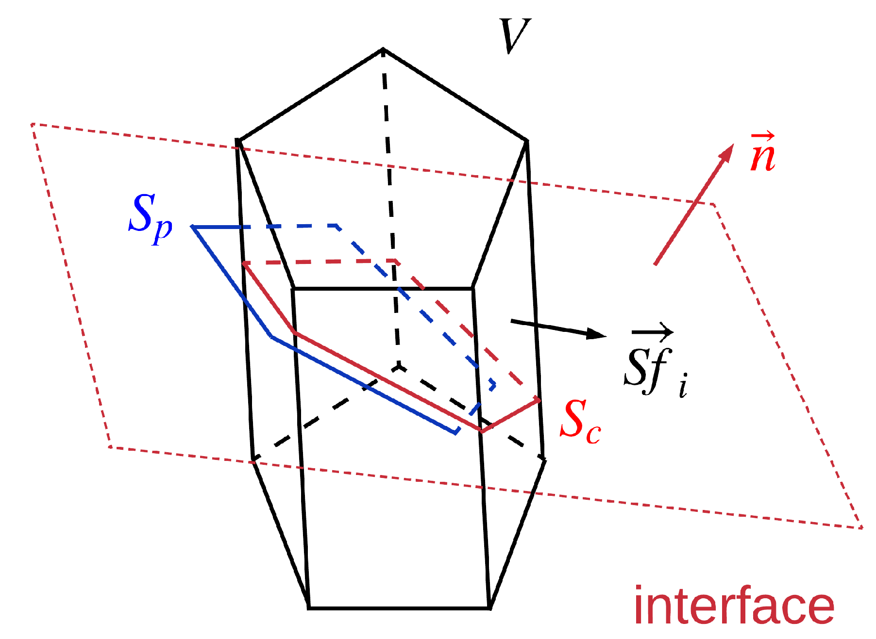
However, Equation (8) only holds for the special case like Figure 1. For a general case where an arbitrary polyhedron is cut by an interface with an arbitrary orientation, as shown in Figure 2, the area of is not easy to calculate due to the fact that interfaces are tracked implicitly in the VOF method. Therefore, a geometric VOF method must be used to reconstruct the interface and to calculate the corresponding area. As mentioned above, this article aims at developing a method suitable for general VOF solvers where the reconstructed interface is not always available. In addition, this interpretation may cause the unboundedness issue of . For instance, when a very tiny is reconstructed, a nonphysically large will be calculated. Therefore, this interpretation was not adopted in this study.
Alternatively, S could also be interpreted as half of the projected area of all the faces on the interface, and this interpretation is denoted by . In Figure 1, only the top and bottom faces have a non-zero projected area on the interface. If we denote these two projected area by and , respectively, we have the following equation:
Using this concept, this is no need to reconstruct the interface geometrically. In addition, this projected area can be easily calculated for any given polyhedral cell, as shown in Figure 2. For any polyhedral cell with volume V, each face has a vector whose direction is the face normal and whose magnitude is the face area. If the cell is in the interfacial region, then the unit normal vector of the interface could be calculated using , and is calculated by:
Then, the length scale for the turbulence damping could be calculated as:
It should be noted that Equation (11) is the definition of . For a general cell shown in Figure 2, does not have an explicit geometric representation as the one used in ANSYS FLUENT [21], i.e., the cell height normal to the interface. Therefore, instead of regarding as a typical cell size or a cell height in a certain direction, it is more proper to refer to as a length scale for the turbulence damping around the interface.
4. Numerical Setup
The experiment conducted by Fabre et al. [4], where air–water stratified flows in a rectangular channel with a 0.001 downward slope were investigated, is often used as the test case for the development of interface damping models. In this study, three flow conditions from the experiment, as shown in Table 1, were investigated.
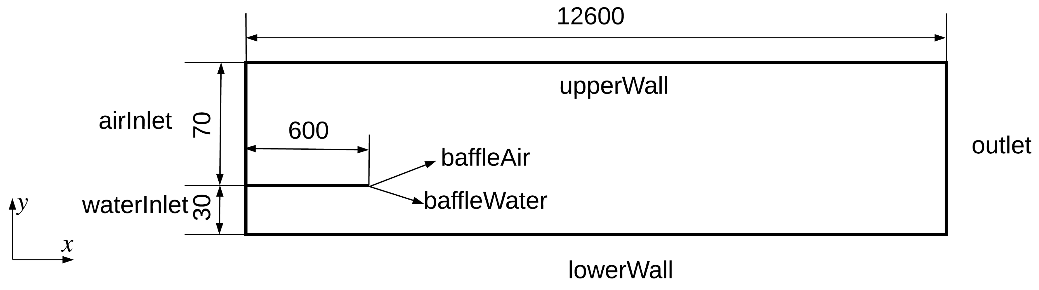
4.1. Computational Domain
A 2D computational domain was constructed as shown in Figure 3. Similarly to the experiment, air and water were supplied via corresponding inlets. These two inlets were assumed to be separated by a zero-thickness 600 mm-long baffle. One reason for making such an assumption is that the details of the baffle were not provided in Fabre et al. [4]. Another reason is that the measuring zone was quite far away from the inlets, indicating that the detailed inlet configurations of the inlet region should only have minor effects on the results of the measuring zone.
4.2. Boundary Conditions
Egorov’s model was implemented in OpenFOAM v1706 with both and . The two-phase system was solved by the VOF solver [22]. The k- model was used for turbulence modeling together with the boundary conditions given in Table 2. All the simulations were run in transient mode, and the data were processed by taking the average value of 50 s after the flow stabilized.
4.3. Mesh
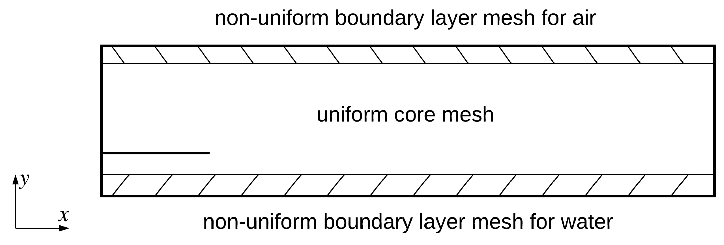
Grid points were divided into three regions in the y direction, i.e., a uniform region in the middle and two non-uniformly-distributed regions near the upperWall and the lowerWall, as shown in Figure 4. These two near-wall regions were designed to minimize the boundary condition effect on the results. This is because if the computational domain is uniformly discretized in the y direction, the thicknesses of the first-layer cells off the walls and other cells in the momentum boundary layers will change with the mesh refinement. This indicates that the wall function approach should be used for a coarse mesh, while a direct-solving approach must be used for a refined mesh. This switching in boundary conditions may introduce additional uncertainties and was not adopted in the present study. Instead, both near-wall regions were always discretized with a very fine mesh to make sure that the same boundary condition was used for all the cases.
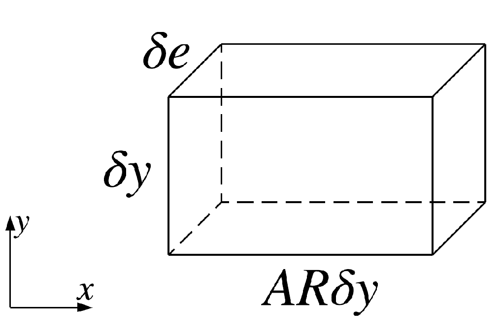
A typical cell in the uniform core mesh is depicted in Figure 5, where the height of the cell is denoted by . By introducing the aspect ratio of the cell, , the length of the cell is calculated as . In OpenFOAM, the 2D mesh should be extruded for one layer of cells in the normal direction of the computational domain. The thickness of this extruded layer, , is usually irrelevant.
5. Advantages of over
Run-250 is used in this section to compare the performance of and . The reason for this selection is that the interface was the least wavy among all the three conditions listed in Table 1. For the sake of clarification, we use and to denote B values that were used for and , respectively.
5.1. Problems with 2D Simulations
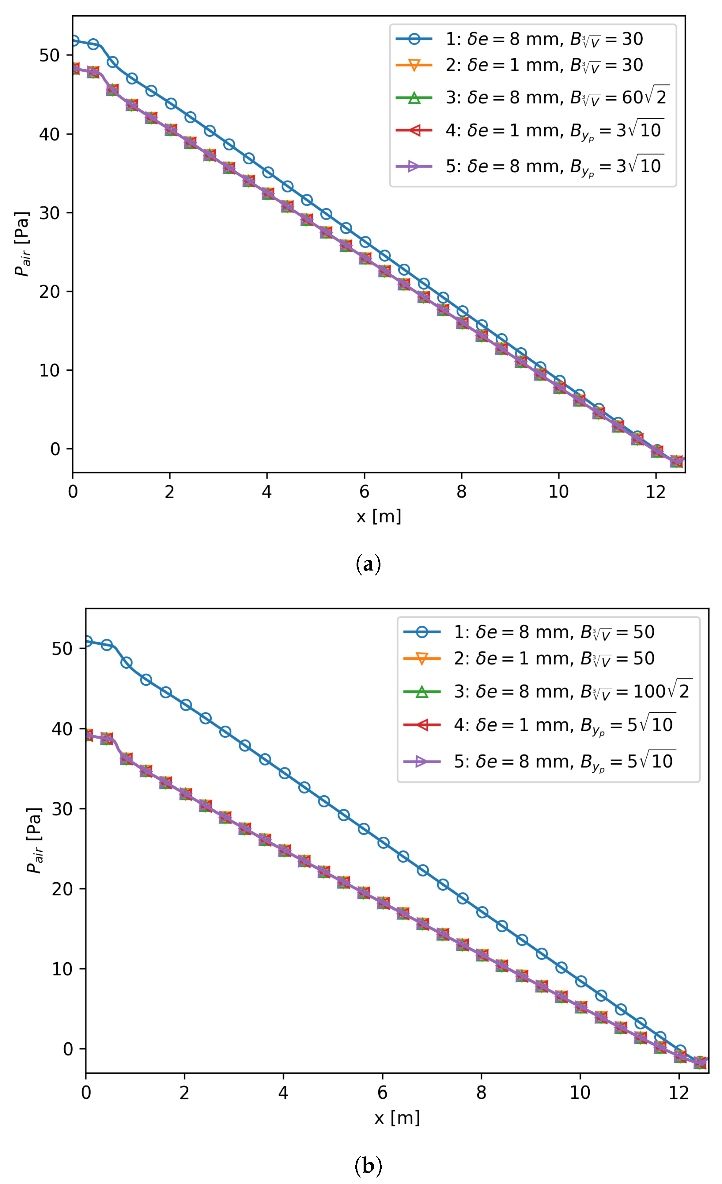
As mentioned above, the one-layer 3D mesh is used in OpenFOAM for 2D simulations. Actually, this strategy is also employed in commercial CFD software like STAR-CCM+ and ANSYS-CFX. The underlying reason is that almost all the codes written for 3D simulations could be easily reused in 2D by simply ignoring the unsolved direction. Therefore, the size of the unsolved dimension, , should not affect the final results. However, if is used in Egorov’s model, the third direction explicitly appears in the governing equation for a 2D flow, which makes the value of dependent on the selection of . In order to prove this statement, a uniform core mesh layout with mm and was created on the plane. Two meshes with mm and mm were generated, respectively. Two reference values, i.e., 30 and 50, were selected to make sure that the following discussion is not based on a special case. If was applied to both meshes, the mesh with mm predicted a higher pressure gradient than the mm mesh did, as shown by Curves 1 and 2 in Figure 6. In the following, we will discuss how to avoid this discrepancy based on the case, and all the discussions hold for the case, as illustrated Figure 6b.
One way to avoid the results being affected by the selection of is to explicitly take the value of into consideration when adding the source term. For instance, in order to match the result of mm with that of mm, two corresponding source terms should be equal, that is:
It is obvious that fluid properties were unchanged in the two cases. Plus, since both meshes had the same 2D layout and solved exactly the same flow, the results should be identical indicating that should be equal in the two cases as well. Therefore, Equation (12) could be rewritten into:
and subsequently, we get:
This implies that by applying to the mesh with mm, the result should match the mesh with mm and . This statement is proven by inspecting Curves 2 and 3 in Figure 6a.
The newly-proposed length scale does not need any information of the value of since its contribution to V is canceled out by its contribution to , as illustrated in Equation (11). For the selected cell with mm, , and mm, we obtained mm. Since the interface was almost flat in the selected case, we could make a rough estimation that mm. It should be noted that all the values were calculated using Equation (11); such an estimation was made to determine the value of , with which the simulation using could give predictions similar to Curve 2 in Figure 6a. According to the calculation, we could get . This means should be used when is used as the length scale, and corresponding results are given by Curves 4 and 5 in Figure 6a. They are close to each other, confirming that is independent of . They are both almost overlapping with Curve 2, meaning that mm and were both good estimations.
5.2. Aspect Ratio Effect
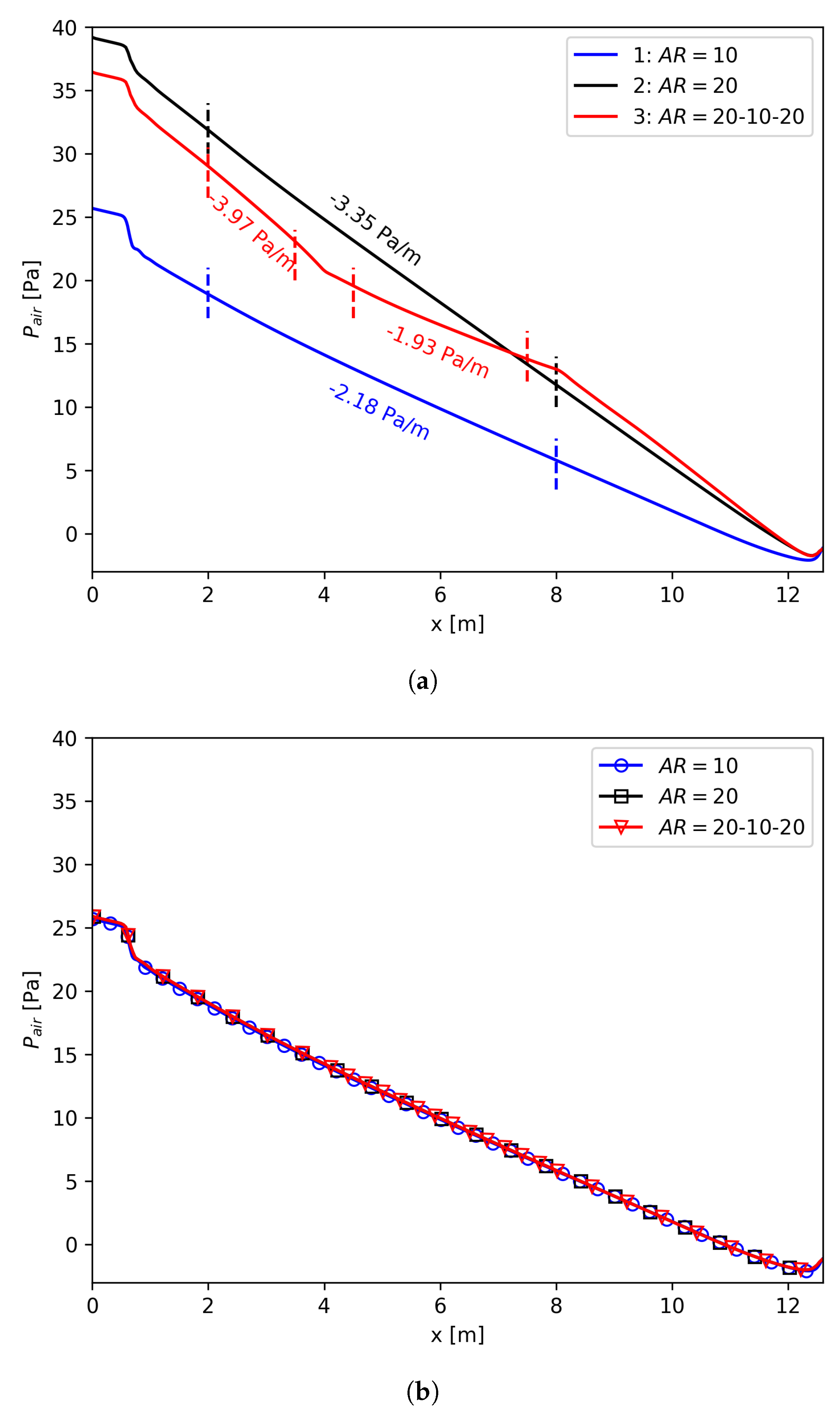
Three meshes with 10, 20, and 20-10-20 were generated to illustrate the limitation of in terms of the aspect ratio of the cell. In all three meshes, mm was used to make the simulation less demanding. AR = 20-10-20 means 10 was used for the middle region, i.e., 4–8 m, of the computational domain, and 20 was used for the other parts of the domain.
The results are shown in Figure 7a. All three curves reach a pressure close to zero at the outlet because the total pressure was set to zero at that location. The large gap between the results obtained by 10 (Curve 1) and 20 (Curve 2) indicates that when using , the value of B is highly dependent on the aspect ratio in the flow direction. This makes the mesh size sensitivity study difficult to conduct.
The 20-10-20 case was designed to show the problem of using when a non-uniform mesh is used for the interfacial region. As illustrated by Curve 3 in Figure 7a, in the 8–12.6 m region, quite close profiles were predicted for the mesh with 20 and the mesh with 20-10-20 because they had the same mesh distribution in this region. Furthermore, such two profiles are almost parallel at the first 4 m due to the same reason. As for the 4.5–7.5 m region, the mesh with 20-10-20 had a pressure gradient similar to that of the mesh with 10. A non-uniform mesh is not uncommon for CFD simulations, e.g., a relatively fine mesh is usually used in the inlet region or a relatively coarse mesh might be used in the outlet region. Using suffers from this non-uniformity of the mesh distribution.
Figure 7a implies that is a poor estimation for since it is so sensitive to the aspect ratio of the interfacial cells. Then, we used the same meshes to test how performed at various aspect ratios. In this part, we will use the same damping factor for all the meshes and try to get pressure profiles close to Curve 1 in Figure 7a. Therefore, we could assume that the cases with and had the same source term:
By assuming that did not change for different meshes, we could get for simulations where was used. The resulting pressure profiles are shown in Figure 7b. It is clear that all three curves are almost overlapping, proving that is insensitive to the aspect ratio of the cells.
5.3. Notes on
We note that the issue of using in 2D simulations could also be categorized into the group of the aspect ratio effect of using . The rationale for discussing it separately in Section 5.1 is that there is an explicit relation like Equation (14) such that we could still use without being affected by the selection of , as illustrated by Curves 2 and 3 in Figure 6. However, in practical simulations, it is not unusual to have non-uniformly-discretized grids; using will suffer from the phenomenon illustrated by Figure 7a, and no obvious correction like Equation (14) exists. In this case, is definitely a much better length scale.
Even though quite regular meshes were used for the above comparisons, once was used as the length scale, the damping factor B still varied dramatically with the grid size. Therefore, selecting as the length scale is one reason causing B to be mesh dependent. By using the newly-proposed length scale , B is much less sensitive to the grid layout in terms of in 2D simulations and the aspect ratio of the interfacial cells.
Similarly to near-wall regions in single-phase flows, the physics near the interface is more dominated by the flow in the normal direction of the interface. From this point of view, it is inappropriate to make Egorov’s model dependent on the mesh size in the direction tangential to the interface. In fact, both in 2D simulations and the aspect ratio of the interfacial cells describe the mesh size effect in the direction tangential to the interface. Therefore, the superiority of over has a solid physical basis. The discussion in Section 5.1 and Section 5.2 is actually motivated by this physical interpretation and eventually justifies this interpretation.
Even though the k- model was used for the turbulence modeling in the present study, the proposed length scale could be used for all other -based turbulence models as well. In addition, Frederix et al. [12] developed a methodology to implement Egorov’s model into -based turbulence models, which makes it straightforward to implement Egorov’s model together with in all the -based models.
6. Further Discussions on Egorov’s Model
With the newly-introduced length scale , more in-depth discussions on Egorov’s model could be carried out based on numerical experiments.
6.1. There Is No Large Enough Value for B
One known issue of Egorov’s model is that the value of B is mesh size dependent. As a result, many values, e.g., 10 [21], 20 [16], 100 [8], 500 [17], and 2500 [10], are used or recommended. Few attempts [12,23] have been made with the hope of finding a large enough value for B that is mesh size independent. The following discussion aims at showing that there is no large enough value for B.
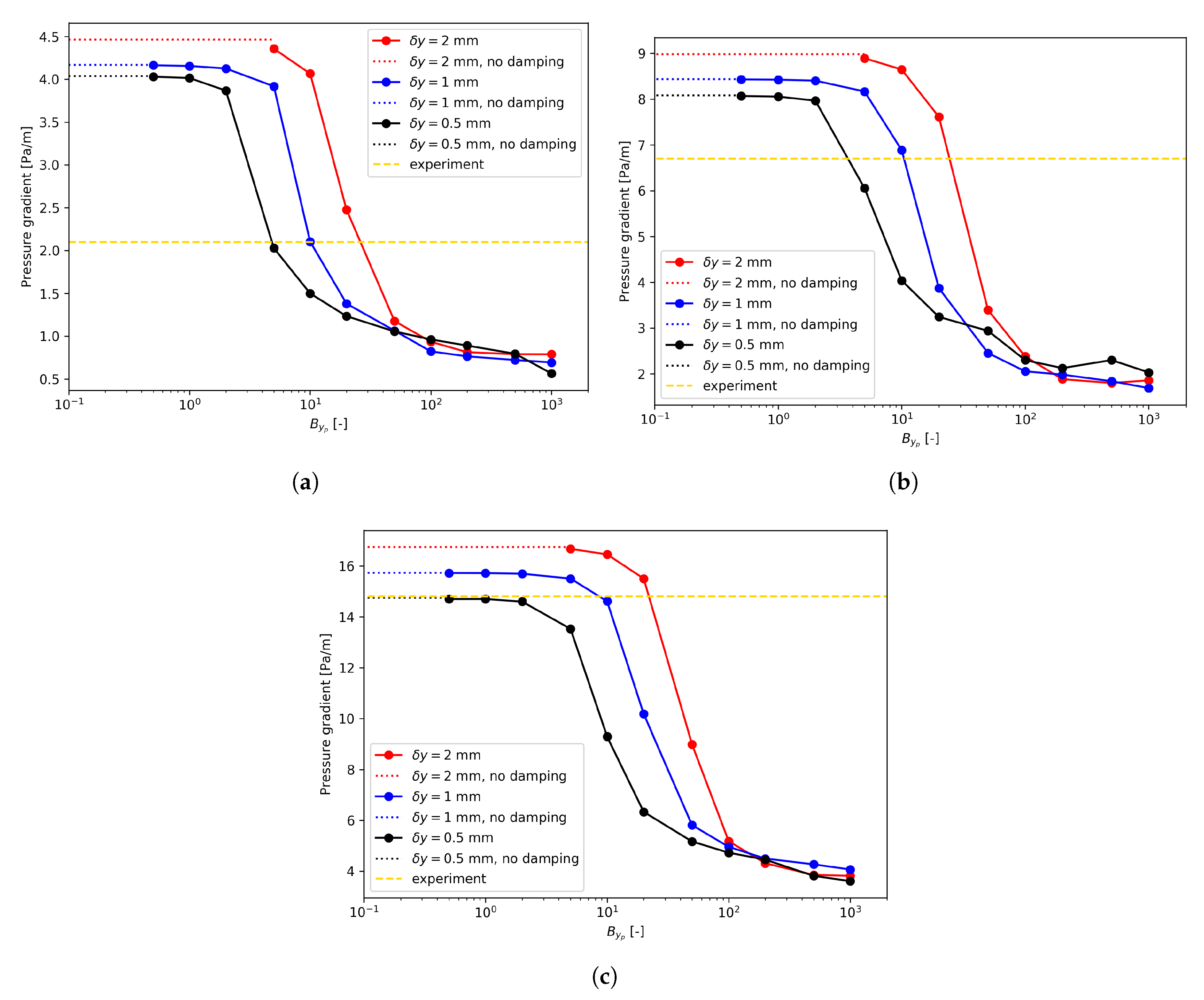
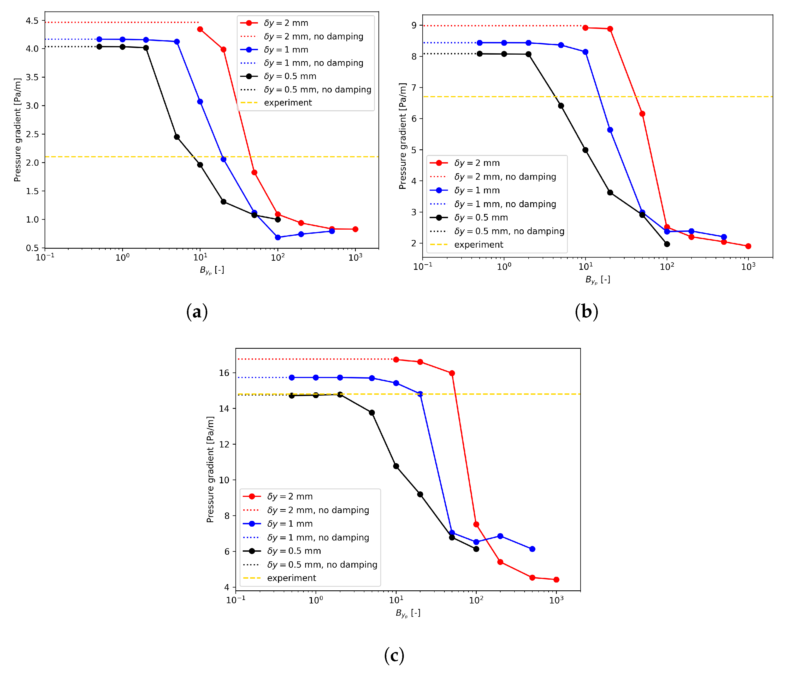
For each flow condition listed in Table 1, there seems to be a region where the value for was large enough, and the pressure drop profiles became rather stable, as shown in Figure 8. Therefore, it seems reasonable to claim that a large enough value, e.g., 1000, could be used for irrespective of the mesh size.
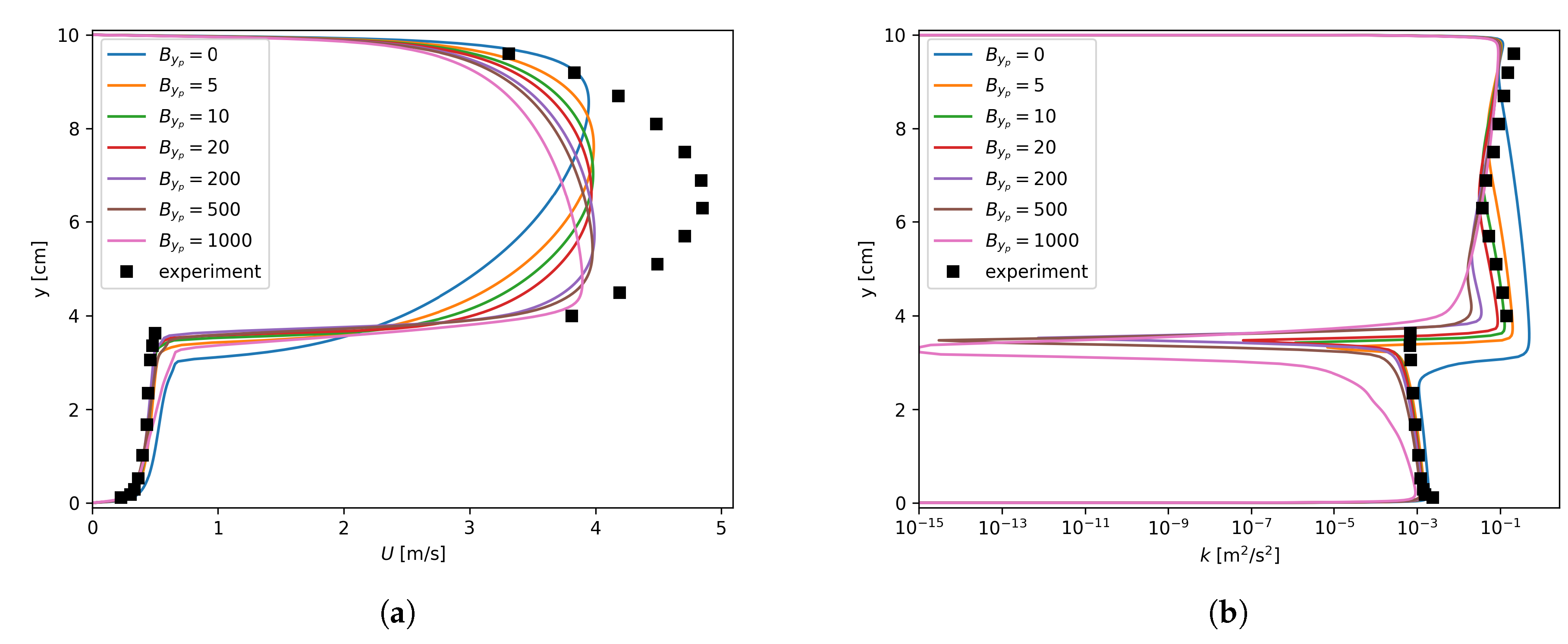
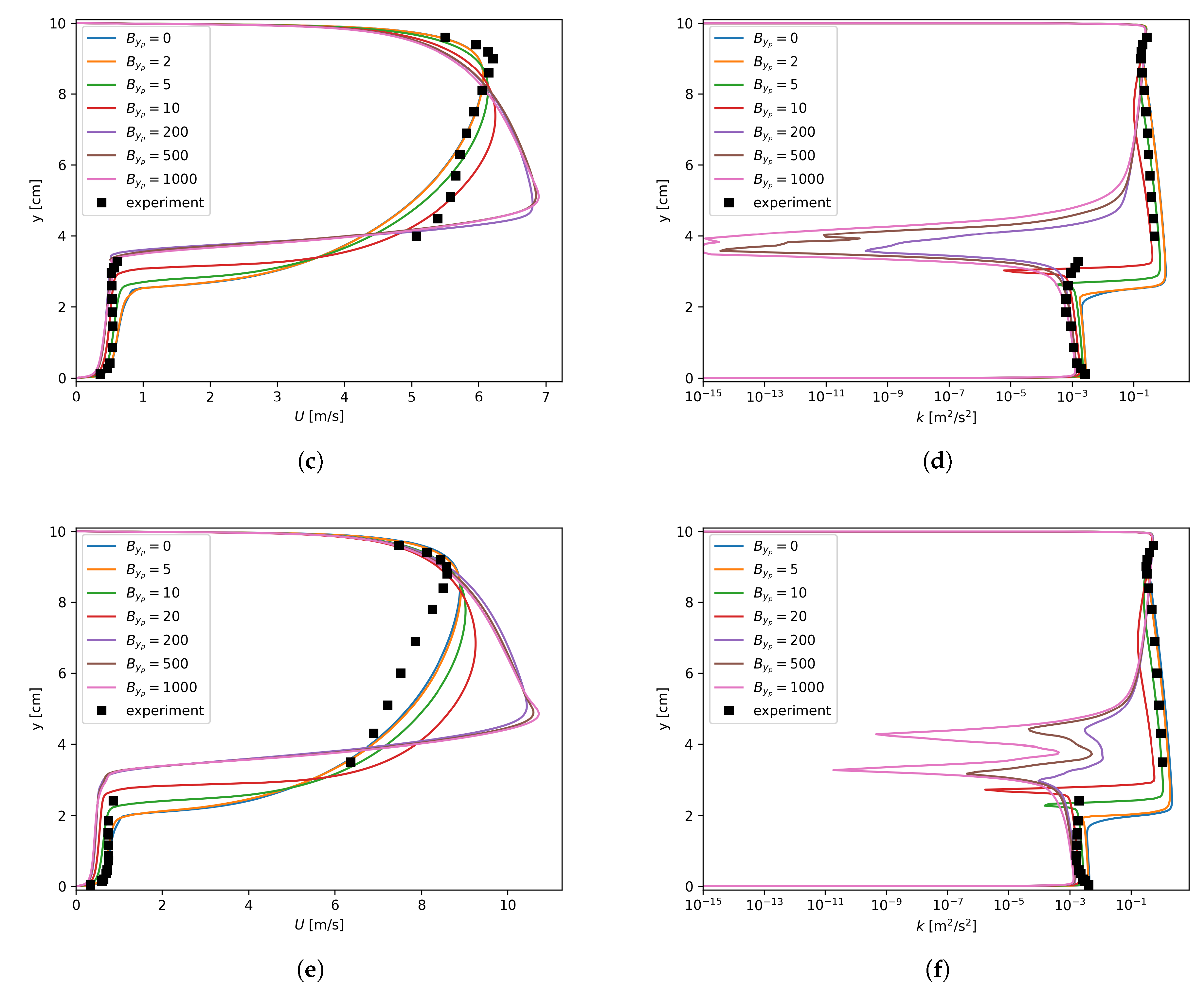
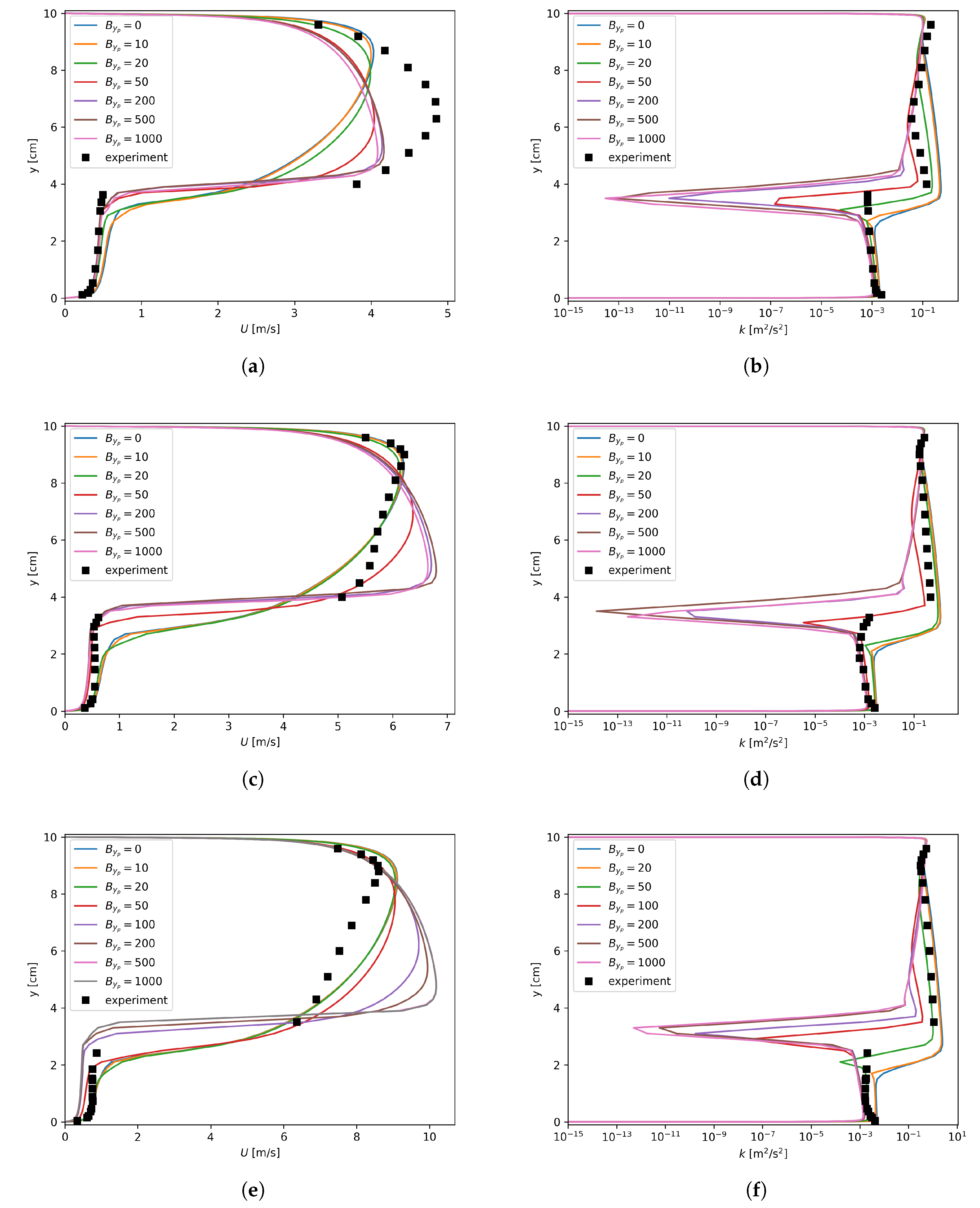
However, this insensitivity is purely numerical and actually does not reflect the physics correctly. In fact, as shown in Figure 8, in the regions where was large enough, the pressure gradients did not converge to the experimental data. On the other hand, when inspecting the profiles of the axial velocity, as shown in Figure 9, the maximum velocities appeared near the interface instead of the upper solid wall. As for the turbulent kinetic energy, extremely small k values could be found around the interface when large values were used for . This indicates that the turbulence damping (described by Equation (6)) was so strong that the turbulence almost died out around the interface. This obviously deviates from the experimental observations shown in Figure 9. In addition, in Figure 9d,f, the profiles are irregular for lager values. The reason is that a large introduces a large source term in the equation. Numerical instability arises when this localized source term is too large. It should be noted that Figure 9 is based on the finest mesh, i.e., mm, and the results for the other two meshes are given in Appendix A.
Lorencez et al. [24] have stressed that k should have a non-zero value around the interface since the velocity fluctuations do not vanish. Plus, the non-zero behavior of k was also observed in the DNS [7]. Therefore, the mesh size-insensitive region does exist for . Unfortunately, such large enough values do not give physical predictions due to the underestimation of the turbulent kinetic energy around the interface.
6.2. Symmetric Treatment for Damping Terms
Another issue with Egorov’s model is that a similar treatment is used for both phases, as shown in Equation (3). This is referred to as the symmetric treatment for damping terms in the sense that turbulence is symmetrically damped for both phases. Therefore, the total source term could be written as:
where subscripts l and g denote the liquid phase and the gas phase, respectively.
It is quite obvious that is always positive, indicating that the turbulence is always damped for the interfacial region. One consequence of this treatment is that k was underestimated for the liquid phase even though an “optimal” value, e.g., 5–10 for mm in terms of the pressure gradient prediction, was used for , as shown in Figure 9b,d,f. Such mispredictions for k in turn affected the results for the velocity field in the liquid phase, as depicted in Figure 9a,c,e.
7. Asymmetric Treatment for Damping Terms
Actually, the symmetric treatment is asymptotically incorrect. In the extreme case where both phases have the same properties, the two-phase flow becomes single-phase. Therefore, the turbulence damping terms should be zero. However, when the symmetric treatment is used, the turbulence damping terms are always positive. In addition, the symmetric treatment is not consistent with the computational observations in the DNS performed by Fulgosi et al. [7], where turbulence on the gas side of the interface was always damped, while on a large portion of the liquid side of the interface, the turbulence was enhanced [25]. Therefore, the interface plays different roles for the liquid and the gas side of the interface, and an asymmetric treatment should be introduced for the turbulence damping terms. We propose the following form of turbulence damping around the interface:
where is a factor to consider the asymmetric damping effect caused by the interface. Obviously, should be negative to model the turbulence enhancement in the liquid phase [7,25]. As is assumed to be constant for the entire interfacial region, we could make the same assumption for . However, if were as mesh size dependent as , the problem would just become more complicated since there is one more free parameter to tune. Therefore, the value of is determined by the following discussion. Recall the property of the interfacial area density shown in Equation (4); we could get the following equation by integrating Equation (17) in the normal direction of the interface:
During the derivation, is assumed to be constant, which is a fairly good assumption when a structured grid is used for a flat interface. However, for meshes with a complex interface structure, this assumption might be poor. As the first trial to show the significance of introducing turbulence enhancement to the liquid side of the interface, we make the following assumption:
The rationale is that, on the one hand, this could guarantee a negative value for such that the turbulence in the liquid phase is enhanced. On the other hand, this treatment actually proposes that, unlike a solid wall, which generates turbulence, the interface acts as a distributor of turbulence. Based on Equations (18) and (19), it is straightforward to get:
This asymmetric treatment was tested against various mesh sizes, flow conditions, and values. The pressure gradient results are shown in Figure 10. The shapes of these curves are very similar to those in Figure 8 especially in the sense that there is always a narrow region where an optimal existed. Similar to the symmetric treatment results, the location of this narrow region is mesh size dependent.
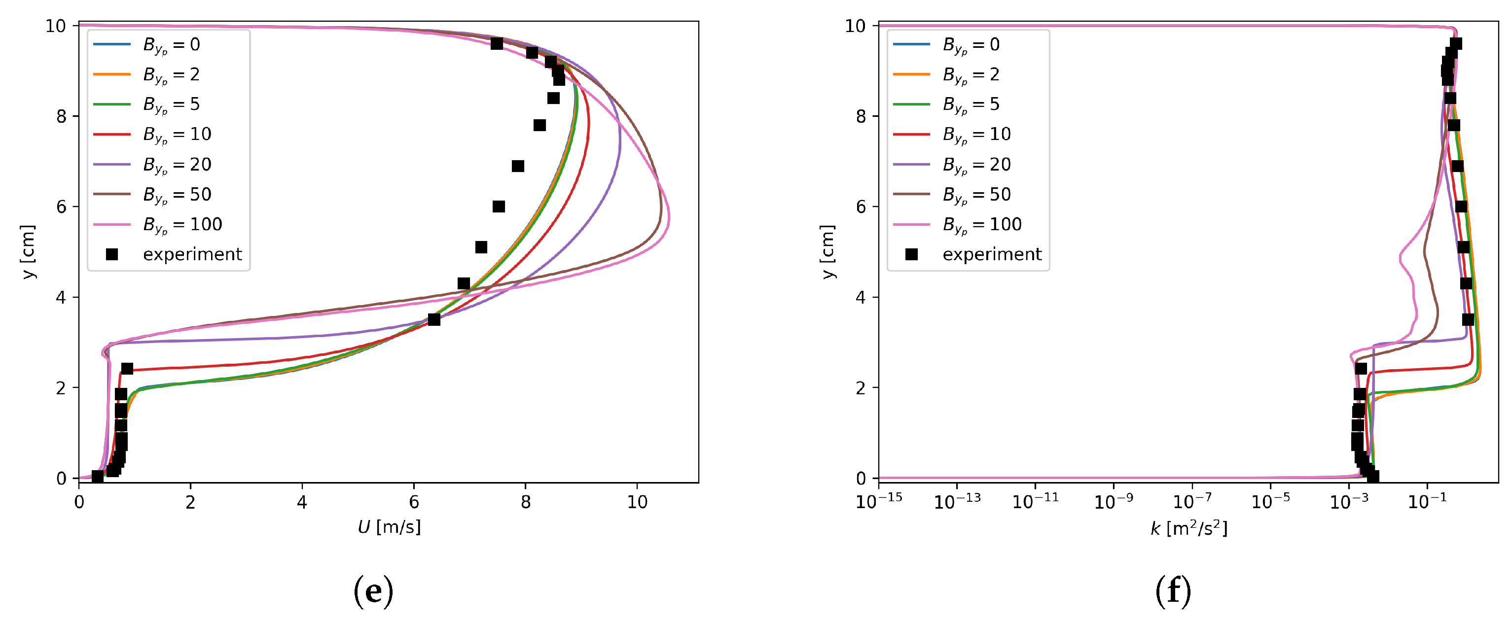
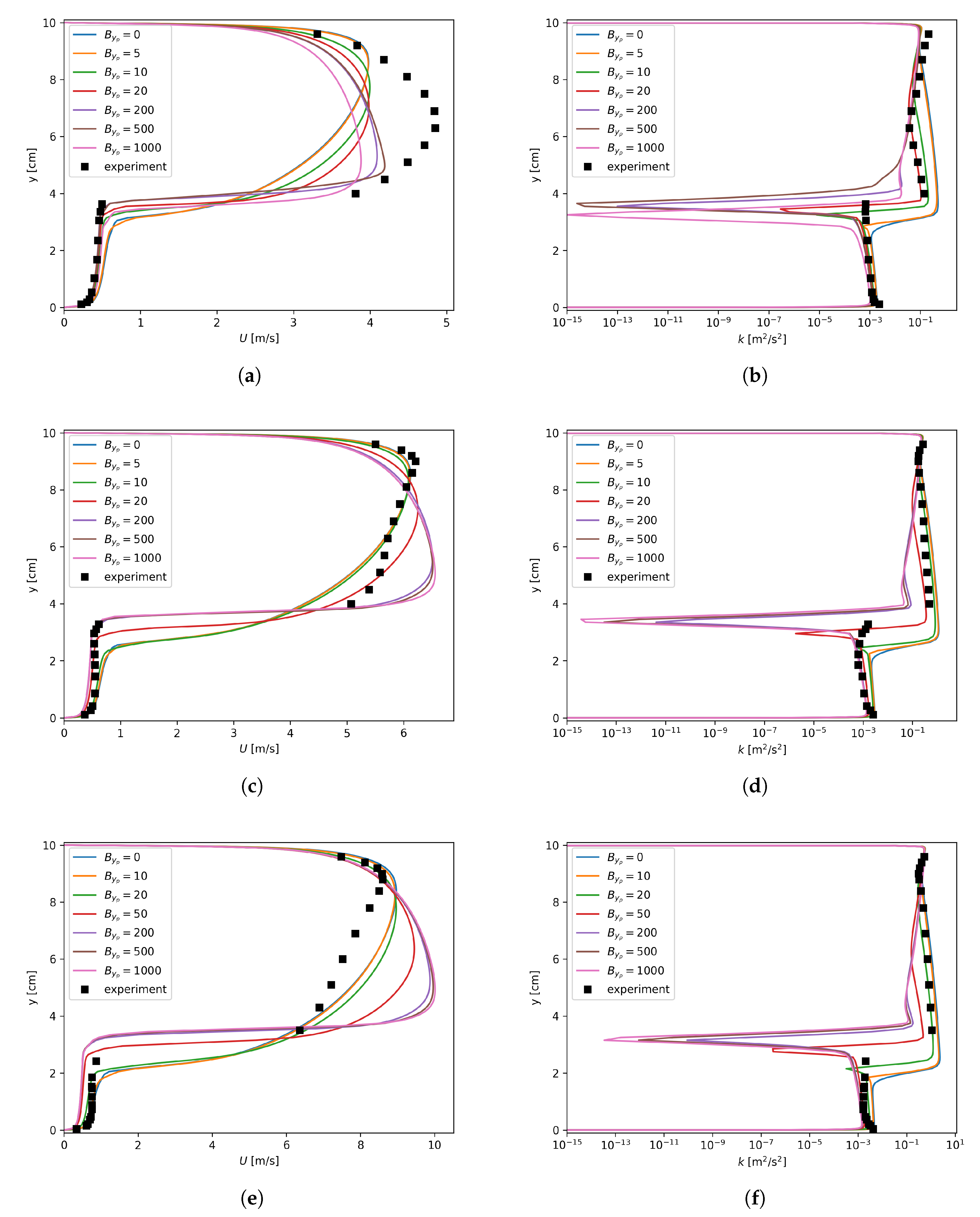
The merits of the proposed asymmetric treatment could be revealed by inspecting the U and k profiles shown in Figure 11. The most eye-catching feature of the asymmetric treatment is the obvious improvement in k profiles around the interface. For instance, when was used for all three flow conditions with mm, k near the interface was no longer underestimated, as shown in Figure 11b,d,f. Consequently, in comparison with Figure 9a,c,e, Figure 11a,c,e have way better agreement with the experimental data for the liquid phase.
8. Conclusions and Outlooks
In this paper, the widely-used Egorov model was further developed by introducing more physics. According to the fact that the near-interface physics is dominated by the flow in the direction normal to the interface, a new length scale, , was proposed to substitute the commonly-used one, . In comparison with , made B independent of the extrusion thickness in 2D simulations and the aspect ratio effect of the mesh. In addition, the calculation of did not require the geometric reconstruction of the interface, making it available to all the VOF methods, as well as the two-fluid approach. An asymmetric treatment was further developed such that turbulence in the liquid phase could be enhanced while turbulence in the gas phase was still damped. With this modification, k profiles around the interface could be physically predicted. Consequently, a better result was calculated for the corresponding velocity profile. Simulations towards other experiments will be carried out to further evaluate the proposed modifications.
Even though made the damping factor B independent of mesh sizes in the direction tangential to the interface, B was still sensitive to the mesh size in the normal direction of the interface. This also directs the future study of the present topic that, in addition to the asymmetric treatment that was already developed in the present work, more physics should be added to the normal direction of the interface. Therefore, it is beneficial to conduct relevant experiments and direct numerical simulations.
Author Contributions
Conceptualization, W.F. and H.A.; methodology, W.F. and H.A.; software, W.F.; validation, W.F.; formal analysis, W.F.; investigation, W.F.; resources, W.F. and H.A.; data curation, W.F.; writing, original draft preparation, W.F.; writing, review and editing, W.F. and H.A.; visualization, W.F.; supervision, H.A.; project administration, H.A.; funding acquisition, W.F. and H.A.
Funding
Wenyuan Fan is financially supported by the China Scholarship Council (CSC, grant No. 201600160035).
Acknowledgments
The simulations were performed on resources provided by the Swedish National Infrastructure for Computing (SNIC) at PDC.
Conflicts of Interest
The authors declare no conflict of interest.
Appendix A. U and k Profiles for Meshes with δy = 2 mm and δy = 1 mm
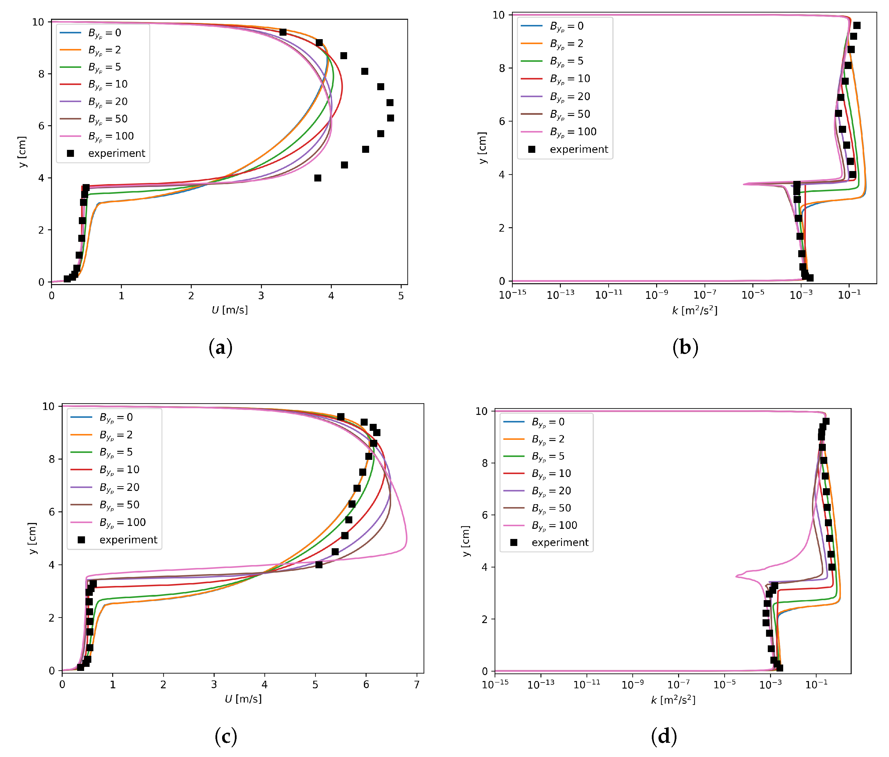
U and k profiles for mm and mm are shown in Figure A1 and Figure A2, respectively. In general, these figures are quite similar to those shown in Figure 9. However, k profiles in these figures are actually of the same pattern and more regular than those in Figure 9. This indicates that the numerical instability was absent for the tested cases with large mesh sizes. One reason is that the magnitude of the source term added to the was inversely proportional to . When a same value was used for , fine meshes were more vulnerable to numerical instabilities. On the other hand, large cells inherently tended to suppress oscillations and avoid instabilities.
Figure A1.
Axial velocity and turbulent kinetic energy dependency on , mm. (a) Run 250, axial velocity; (b) Run 250, k; (c) Run 400, axial velocity; (d) Run 400, k; (e) Run 600, axial velocity; (f) Run 600, k.
Figure A1.
Axial velocity and turbulent kinetic energy dependency on , mm. (a) Run 250, axial velocity; (b) Run 250, k; (c) Run 400, axial velocity; (d) Run 400, k; (e) Run 600, axial velocity; (f) Run 600, k.

Figure A2.
Axial velocity and turbulent kinetic energy dependency on , mm. (a) Run 250, axial velocity; (b) Run 250, k; (c) Run 400, axial velocity; (d) Run 400, k; (e) Run 600, axial velocity; (f) Run 600, k.
Figure A2.
Axial velocity and turbulent kinetic energy dependency on , mm. (a) Run 250, axial velocity; (b) Run 250, k; (c) Run 400, axial velocity; (d) Run 400, k; (e) Run 600, axial velocity; (f) Run 600, k.

References
- Hirt, C.; Nichols, B. Volume of fluid (VOF) method for the dynamics of free boundaries. J. Comput. Phys. 1981, 39, 201–225. [Google Scholar] [CrossRef]
- Ishii, M.; Mishima, K. Two-fluid model and hydrodynamic constitutive relations. Nucl. Eng. Des. 1984, 82, 107–126. [Google Scholar] [CrossRef]
- Sussman, M.; Smereka, P.; Osher, S. A Level Set Approach for Computing Solutions to Incompressible Two-Phase Flow. J. Comput. Phys. 1994, 114, 146–159. [Google Scholar] [CrossRef]
- Fabre, J.; Suzanne, C.; Masbernat, L. Experimental Data Set No. 7: Stratified Flow, Part I: Local Structure. Multiph. Sci. Technol. 1987, 3, 285–301. [Google Scholar] [CrossRef]
- Rashidi, M.; Banerjee, S. The effect of boundary conditions and shear rate on streak formation and breakdown in turbulent channel flows. Phys. Fluids A Fluid Dyn. 1990, 2, 1827–1838. [Google Scholar] [CrossRef]
- Lombardi, P.; De Angelis, V.; Banerjee, S. Direct numerical simulation of near-interface turbulence in coupled gas-liquid flow. Phys. Fluids 1996, 8, 1643–1665. [Google Scholar] [CrossRef]
- Fulgosi, M.; Lakehal, D.; Banerjee, S.; De Angelis, V. Direct numerical simulation of turbulence in a sheared air-water flow with a deformable interface. J. Fluid Mech. 2003, 319–345. [Google Scholar] [CrossRef]
- Egorov, Y. Validation of CFD codes with PTS-relevant test cases. In 5th Euratom Framework Programme ECORA Project; European Commission: Brussels, Belgium, 2004; pp. 91–116. [Google Scholar]
- Liovic, P.; Lakehal, D. Multi-physics treatment in the vicinity of arbitrarily deformable gas-liquid interfaces. J. Comput. Phys. 2007, 222, 504–535. [Google Scholar] [CrossRef]
- Lo, S.; Tomasello, A. Recent progress in CFD modelling of multiphase flow in horizontal and near-horizontal pipes. In Proceedings of the 7th North American Conference on Multiphase Technology, BHR Group, Banff, AB, Canada, 2–4 June 2010; pp. 209–219. [Google Scholar]
- Thompson, C.P.; Sawko, R. Interface Turbulence Treatments in RANS Models of Stratified Gas/Liquid Flows. In Proceedings of the ASME 2012 International Mechanical Engineering Congress and Exposition, Houston, TX, USA, 9–15 November 2012; pp. 621–626. [Google Scholar]
- Frederix, E.; Mathur, A.; Dovizio, D.; Geurts, B.; Komen, E. Reynolds-averaged modeling of turbulence damping near a large-scale interface in two-phase flow. Nucl. Eng. Des. 2018, 333, 122–130. [Google Scholar] [CrossRef]
- Qiu, G.; Wei, X.; Cai, W.; Jiang, Y. Development and validation of numerical model of condensation heat transfer and frictional pressure drop in a circular tube. Appl. Therm. Eng. 2018, 143, 225–235. [Google Scholar] [CrossRef]
- Bristot, A.; Morvan, H.P.; Simmons, K.; Klingsporn, M. Effect of turbulence damping in vof simulation of an aero-engine bearing chamber. In Proceedings of the ASME Turbo Expo 2017, Charlotte, NC, USA, 26–30 June 2017; Volume 2B-2017, pp. 1–10. [Google Scholar] [CrossRef]
- Elhanafi, A.; Fleming, A.; Leong, Z.; Macfarlane, G. Effect of RANS-based turbulence models on nonlinear wave generation in a two-phase numerical wave tank. Prog. Comput. Fluid Dyn. 2017, 17, 141. [Google Scholar] [CrossRef]
- Fan, W.; Li, H.; Anglart, H. Numerical investigation of spatial and temporal structure of annular flow with disturbance waves. Int. J. Multiph. Flow 2019, 110, 256–272. [Google Scholar] [CrossRef]
- Gada, V.H.; Tandon, M.P.; Elias, J.; Vikulov, R.; Lo, S. A large scale interface multi-fluid model for simulating multiphase flows. Appl. Math. Model. 2017, 44, 189–204. [Google Scholar] [CrossRef]
- Höhne, T.; Mehlhoop, J.P. Validation of closure models for interfacial drag and turbulence in numerical simulations of horizontal stratified gas-liquid flows. Int. J. Multiph. Flow 2014, 62, 1–16. [Google Scholar] [CrossRef]
- Menter, F.R. Two-equation eddy-viscosity turbulence models for engineering applications. AIAA J. 1994, 32, 1598–1605. [Google Scholar] [CrossRef] [Green Version]
- Menter, F.R.; Esch, T. Elements of Industrial Heat Transfer Predictions. In Proceedings of the 16th Brazilian Congress of Mechanical Engineering, Uberlandia, Brazil, 26–30 November 2001; pp. 117–127. [Google Scholar] [CrossRef]
- ANSYS Inc. ANSYS FLUENT 18.0 Theory Guide; ANSYS Inc.: Cannonsburg, PA, USA, 2017. [Google Scholar]
- Fan, W.; Anglart, H. vFoam: A new set of volume of fluid solvers for turbulent isothermal multiphase flows. arXiv 2018, arXiv:1811.12580. [Google Scholar]
- Gada, V.; Punde, P.; Tandon, M.P.; Vikulov, R. Role of Turbulence Damping at the Gas-Liquid Interface. In Proceedings of the 9th International Conference on Multiphase Flow, Firenze, Italy, 22–27 May 2016. [Google Scholar]
- Lorencez, C.; Nasr-Esfahany, M.; Kawaji, M.; Ojha, M. Liquid turbulence structure at a sheared and wavy gas-liquid interface. Int. J. Multiph. Flow 1997, 23, 205–226. [Google Scholar] [CrossRef]
- Lakehal, D. Status and future developments of Large-Eddy Simulation of turbulent multi-fluid flows (LEIS and LESS). Int. J. Multiph. Flow 2018, 104, 322–337. [Google Scholar] [CrossRef]
Figure 1.
A cuboid is cut by an interface (red dotted surface), and their common surface has an area of S. The interface, with being its unit normal vector, is perpendicular to four inter-parallel edges.
Figure 1.
A cuboid is cut by an interface (red dotted surface), and their common surface has an area of S. The interface, with being its unit normal vector, is perpendicular to four inter-parallel edges.

Figure 2.
A polyhedron with volume V is cut by an interface with being its unit normal vector. Each face of the polyhedron has a surface area vector whose direction is the face normal and whose magnitude is the face area. is the common surface of the polyhedron and the interface. is half of the projected area.

Figure 3.
Sketch of the computational domain (units in mm, not to scale).

Figure 4.
Two non-uniform boundary layer mesh regions are created for the upperWall and lowerWall to ensure that these regions are always resolved by a high-quality mesh. The uniform core mesh guarantees that cells in the interfacial region are always of the same size.
Figure 4.
Two non-uniform boundary layer mesh regions are created for the upperWall and lowerWall to ensure that these regions are always resolved by a high-quality mesh. The uniform core mesh guarantees that cells in the interfacial region are always of the same size.

Figure 5.
A typical cell in the uniform core mesh.

Figure 6.
Axial pressure profile comparisons for meshes with mm and mm. When is used, the meshes with mm (Curve 2) predict a higher pressure gradient than that of mm (Curve 1). By setting for the mesh with mm (Curve 3) or using for both meshes (Curves 4 and 5), the predicted pressure gradients are close to Curve 1. (a) ; (b) .

Figure 7.
Axial pressure profiles for meshes with 10, 20, and 20-10-20. Top: is sensitive to the aspect ratio of the cells; it performs worse for non-uniformly-distributed cells. Bottom: shows much less dependency on the aspect ratio of the cells. (a) ; (b) .
Figure 7.
Axial pressure profiles for meshes with 10, 20, and 20-10-20. Top: is sensitive to the aspect ratio of the cells; it performs worse for non-uniformly-distributed cells. Bottom: shows much less dependency on the aspect ratio of the cells. (a) ; (b) .

Figure 8.
Pressure gradient dependency on . (a) Run 250; (b) Run 400; (c) Run 600.

Figure 9.
Axial velocity and turbulent kinetic energy dependency on , mm. (a) Run 250, U; (b) Run 250, k; (c) Run 400, U; (d) Run 400, k; (e) Run 600, U; (f) Run 600, k.
Figure 9.
Axial velocity and turbulent kinetic energy dependency on , mm. (a) Run 250, U; (b) Run 250, k; (c) Run 400, U; (d) Run 400, k; (e) Run 600, U; (f) Run 600, k.


Figure 10.
Pressure gradient dependency on with . (a) Run 250; (b) Run 400; (c) Run 600.

Figure 11.
Axial velocity and turbulent kinetic energy dependency on with , mm. (a) Run 250, U; (b) Run 250, k; (c) Run 400, U; (d) Run 400, k; (e) Run 600, U; (f) Run 600, k.
Figure 11.
Axial velocity and turbulent kinetic energy dependency on with , mm. (a) Run 250, U; (b) Run 250, k; (c) Run 400, U; (d) Run 400, k; (e) Run 600, U; (f) Run 600, k.


Table 1.
Flow conditions and experimental data [4].
Table 1.
Flow conditions and experimental data [4].
| Run Reference | Air Average Velocity (m/s) | Water Average Velocity (m/s) | Pressure Gradient (Pa/m) |
|---|---|---|---|
| 250 | 3.66 | 0.395 | 2.10 |
| 400 | 5.50 | 0.476 | 6.70 |
| 600 | 7.56 | 0.698 | 14.80 |
Table 2.
Boundary conditions.
| airInlet | waterInlet | outlet | upperWall | lowerWall | baffleAir | baffleWater | |
|---|---|---|---|---|---|---|---|
| U | mappedC | mappedC | advective | no slip | no slip | no slip | no slip |
| fixed flux | fixed flux | fixed total pressure | fixed flux | fixed flux | fixed flux | fixed flux | |
| k | mappedN | mappedN | wall function | wall function | |||
| mappedN | mappedN | wall function | wall function | wall function | wall function |
mapped condition with the constraint on the average value; mapped condition without constraints; there is a bug in in the official release of OpenFOAM v1706, and it was fixed in the present study.
© 2019 by the authors. Licensee MDPI, Basel, Switzerland. This article is an open access article distributed under the terms and conditions of the Creative Commons Attribution (CC BY) license (http://creativecommons.org/licenses/by/4.0/).
Share and Cite
MDPI and ACS Style
Fan, W.; Anglart, H. Progress in Phenomenological Modeling of Turbulence Damping around a Two-Phase Interface. Fluids 2019, 4, 136. https://0-doi-org.brum.beds.ac.uk/10.3390/fluids4030136
AMA Style
Fan W, Anglart H. Progress in Phenomenological Modeling of Turbulence Damping around a Two-Phase Interface. Fluids. 2019; 4(3):136. https://0-doi-org.brum.beds.ac.uk/10.3390/fluids4030136
Chicago/Turabian StyleFan, Wenyuan, and Henryk Anglart. 2019. "Progress in Phenomenological Modeling of Turbulence Damping around a Two-Phase Interface" Fluids 4, no. 3: 136. https://0-doi-org.brum.beds.ac.uk/10.3390/fluids4030136