A New Wall Model for Large Eddy Simulation of Separated Flows


Institute for Polymers and Composites, Department of Polymer Engineering, Campus of Azurém, University of Minho, 4800-058 Guimarães, Portugal
Fluids 2019, 4(4), 197; https://0-doi-org.brum.beds.ac.uk/10.3390/fluids4040197
Submission received: 14 September 2019
/
Revised: 14 November 2019
/
Accepted: 19 November 2019
/
Published: 28 November 2019
(This article belongs to the Special Issue Recent Numerical Advances in Fluid Mechanics)
Abstract
:The aim of this work is to propose a new wall model for separated flows which is combined with large eddy simulation (LES) of the flow field in the whole domain. The model is designed to give reasonably good results for engineering applications where the grid resolution is generally coarse. Since in practical applications a geometry can share body fitted and immersed boundaries, two different methodologies are introduced, one for body fitted grids, and one designed for immersed boundaries. The starting point of the models is the well known equilibrium stress model. The model for body fitted grid uses the dynamic evaluation of the von Kármán constant of Cabot and Moin (Flow, Turbulence and Combustion, 2000, 63, pp. 269–291) in a new fashion to modify the computation of shear velocity which is needed for evaluation of the wall shear stress and the near-wall velocity gradients based on the law of the wall to obtain strain rate tensors. The wall layer model for immersed boundaries is an extension of the work of Roman et al. (Physics of Fluids, 2009, 21, p. 101701) and uses a criteria based on the sign of the pressure gradient, instead of one based on the friction velocity at the projection point, to construct the velocity under an adverse pressure gradient and where the near-wall computational node is in the log region, in order to capture flow separation. The performance of the models is tested over two well-studied geometries, the isolated two-dimensional hill and the periodic two-dimensional hill, respectively. Sensitivity analysis of the models is also performed. Overall, the models are able to predict the first and second order statistics in a reasonable way, including the position and extension of the downward separation region.
1. Introduction
Wall bounded turbulent flows, especially at high Reynolds numbers, require a high resolution near the wall, because of the need to solve the thin viscous sub-layer [1,2,3]. In LES, this resolution is comparable with that required by direct numerical simulation (DNS). As far as Reynolds number increases, the cost of a wall-resolving LES augments with (for a discussion, see Piomelli and Balaras [1]). Moreover, for applications where wall roughness is the rule rather than the exception, it is not feasible to describe the wall boundary in a deterministic sense.
The most practical way of simulating a wall-bounded, high Reynolds number flow, is to consider coarse grid, and model the wall shear stress with a wall function. This function is designed to mimic the stress induced by the wall, produced by the adherence condition and ruled by the turbulent field. Several wall layer models have been developed in the past (for a discussion, see Piomelli and Balaras [1] and Piomelli [2]). They are designed to work under certain conditions, and in particular they may suffer in the presence of massive separation. This subject is still challenging for improvement.
In equilibrium stress models, the grid is generated in such a way that the first near-wall computational node is placed in the log region of the boundary layer. So, based on the law of the wall, the instantaneous or mean horizontal velocity can be fitted to determine the wall stress. These models are valid only under the equilibrium assumption and work for both smooth and rough walls.
Deardorff [4] and Schumann [5] first used the concept of wall layer modeling in conjunction with LES. Applying LES on plane channel flow and annuli at large Reynolds numbers, they assumed the existence of an equilibrium-stress layer near the wall and used the outer flow velocity to calculate the wall stress based on the logarithmic law.
Deardorff [4] considered a second order velocity derivative in vertical direction and forced plane averaged stream-wise and spanwise velocity gradients to follow logarithmic law. Schumann [5] obtained the plane averaged wall shear stress from plane averaged velocity at the first grid point, using the iterative method so that the shear velocity is computed from the law of the wall from the averaged velocity. These methods are the least expensive wall layer models. They also provide roughness corrections easily from the logarithmic law modification, which is an important feature in environmental and oceanographic flows. The models suffer in cases of marginal separation, or strong pressure gradient [2].
In zonal approaches (two-layer models, TLMs), stress derives from the solution of a separate set of equations on a finer mesh close to the wall. This model was proposed by Balaras and Benocci [6] who applied turbulent boundary layer equations inside the boundary layer (inner layer) and LES on the outer region. In this model, a finer grid is considered between the wall and the first computational node of the coarser grid. A uniform pressure field is applied from LES for the inner layer, and velocity field from LES is considered at the edge of the Reynolds Averaged Navier-Stokes (RANS) region as its boundary condition. The coupling between the inner and outer regions of the boundary layer is weak, and these models have problems when a perturbation extends from the wall to the outer layer. Balaras and Benocci [6] used an algebraic eddy viscosity to parametrize the near-wall region. In addition to plane channel flow, this method was tested on square ducts and also rotating channel, the cases in which equilibrium stress model was not valid or even failed; this method showed a good accuracy in simulating these flows. These methods, able to simulate equilibrium as well as non-equilibrium flows were not designed to deal with separated flows.
Cabot [7] applied this approach to simulate flow over a backward-facing step with only grid points fewer than those used in former wall-resolved LES. He found that stream-wise pressure gradient has an important effect in boundary layers of TLMs. In this case, mean velocity and skin friction coefficient were predicted well; however, the backward-facing step is just a simple case where separation is induced by the sharp discontinuity in the streamlines.
Cabot and Moin [8] used the wall layer model in conjunction with LES to simulate the flow over a backward-facing step. They considered a zonal approach using thin boundary layer equations (TBLEs) in the inner layer and LES (dynamic SGS model) in the outer region. This way, they were able to use eight uniform cells from the bottom of the wall up to half the height of the step, greatly reducing the total number of cells with respect to a stretched-grid case previously used for the wall-resolved LES.
Finally, in hybrid methods, a single grid is used and the turbulence models are different in inner and outer layers. Detached eddy simulation (DES) is a hybrid approach proposed by Spalart et al. [9] as a method to compute massive separation. According to DES, a stretched grid is used close to the wall to resolve the boundary layer. RANS is applied in the inner and LES in the outer region.
Since there is no zonal interface between the inner and the outer layer, velocity profile is smooth everywhere. Some weaknesses of this method are logarithmic layer mismatch between the two regions and high grid resolution dependency near the wall. In addition, time and length scales of the eddies in the inner layer (modelled by unsteady RANS equations with the Spalart-Allmaras 1-equation turbulent model) are much larger than those computed in the outer region by LES; this leads to much lower resolved stress by LES than the modelled stress (by RANS) at the RANS/LES interface and even farther Piomelli [2]. A review of DES and the two modifications of it, which are delayed detached eddy simulation (DDES) and improved delayed detached eddy simulation (IDDES), can be seen in Mockett et al. [10].
The total shear stress in plane channel flow only depends on the distance from the wall, therefore a reduction of eddy viscosity farther than the RANS/LES interface affects the velocity profile and generates a high gradient at the transition into LES region. This phenomenon is called the DES buffer layer. To eliminate this, Keating and Piomelli [11] added stochastic force in the interface region to accelerate resolved eddy generation, thus obtaining better results. Temmerman et al. [12] also computed the constant required to calculate eddy viscosity in the RANS region in such a way to equate the eddy viscosity of RANS and LES at the interface of their hybrid RANS/LES application.
While the hybrid RANS/LES methods work satisfactorily in flows with instabilities such as those with adverse pressure gradient and concave curvature, they are weak in attached flows, and, in general, in flows with a low level of instability; in these cases a false merging region may appear at the RANS/LES interface. Since the grid near the wall must be resolved, they are the most expensive ones in the wide family of wall layer models. In addition to the three main wall layer frameworks herein discussed, there are other models which are not mentioned here.
The near-wall modelisation must be implemented in the algorithms that solve the governing equations using different strategies. A body fitted (also called boundary fitted) case is the case in which a grid is generated to follow the geometry. Since the grid boundaries coincide with the solid surface of a solid body, boundary conditions are imposed on certain grid nodes or cell faces. This facilitates the computation of all the vectorial quantities as well as of their gradients.
In complex geometry, where a structured grid can hardly follow the boundary complexities, alternative approaches must be employed. Among others, the immersed boundary method (IBM) has proved to be simple, effective and accurate (Mittal and Iaccarino [13]). The domain grid can be either Cartesian or curvilinear. In this approach the cells are cut by the solid surface and the cell boundaries in the general cases do not coincide with the solid boundaries. Hence the fluxes at the solid surfaces are difficult to define. Finally, the velocities in near-wall computational nodes are reconstructed and thus a local frame of reference must be introduced at each near-wall node to identify directions normal and tangential to the immersed boundary.
A number of papers have been published discussing different implementations of immersed boundary methods (see Mittal and Iaccarino [13]). Among others, Roman et al. [14] extended IBM to the general case of curvilinear coordinates, and simulated both steady and unsteady flows in complex geometric configurations showing the flexibility of this methodology when compared to the Cartesian counterpart. However, few papers have dealt with the development of wall layer models in conjunction with immersed boundaries. This is a matter of great importance when flows at a high Reynolds number over complex geometry must be simulated.
Tessicini et al. [15] applied wall layer model LES in the presence of immersed boundaries to simulate the flow past a , asymmetric trailing edge of a model hydrofoil. The Reynolds number, based on free stream velocity and the hydrofoil chord (C), was chosen equal to . They used turbulent boundary layer equations for modelling the wall layer. In general, their results were good, although they had a deviation at the second off-the-wall node, which was considered as the outer boundary for the wall model. This discrepancy was sensitive to the distance of the second node from the wall, and was more evident where the distance was larger.
Posa and Balaras [16] proposed a new near-wall reconstruction model to account for the lack of resolution and provided correct wall shear stress and hydrodynamic forces. They used a zonal approach (TLM), boundary layer equations with a finer grid in the near-wall region (called in this case the full boundary layer FBL) and LES in the outer region. They validated their model to simulate flow around a cylinder and a sphere.
Then, they considered a coarser grid, and set one node inside the boundary layer and neglected the advective term in boundary layer equations. This was justified by the fact that, if the first point off the wall is located inside the boundary layer, neglecting this term does not provide significant errors. They assumed a constant pressure gradient between the first and second nodes, and obtained tangential velocity with two approaches: The reduced diffusion model (RDM) and the hybrid reconstruction method (HRM). The Reynolds number in the cylinder case was based on free stream velocity and the cylinder diameter, and in the sphere was . The pressure coefficient for all cases was predicted well, while the skin friction was underestimated in all cases, but an improvement was observed using RDM and HRM in comparison with linear reconstruction. The prediction of separation was also improved a lot using these two approaches.
Chen et al. [17] also proposed a wall layer model based on turbulent boundary layer equations at high Reynolds numbers for implicit LES in the presence of immersed boundaries. First, they tested it on a turbulent channel flow in the range of Reynolds numbers (based on shear velocity) from to . They used a minimum of 20 cells inside the boundary layer for lower Reynolds numbers and 40 cells for higher values. Inside the boundary layer (inner region), the pressure gradient and friction are dominant, thus advection is neglected in cases where there are slow changes in wall parallel direction and sharp changes in wall normal direction. The fact that the changes in wall normal direction are sharper at higher Reynolds numbers requires more resolution for capturing the flow in this direction.
They also simulated flow over a backward-facing step at a Reynolds number based on the step height in a Cartesian grid. Finally they simulated the flow over periodic hills at = 10,595 based on hill height, using different resolutions, and they obtained comparatively good results. To summarize, different models have an acceptable accuracy under some special conditions; therefore, more general models are needed to work well in different situations characterized by attached as well as separated flow conditions.
In the present study, attempts are made to overcome some of the difficulties mentioned above, proposing wall layer model to be used in conjunction with LES, suited for both attached and detached flows. Since in engineering applications a combination of body fitted solid walls and immersed boundaries is often employed, a comprehensive model must include the two aspects. Here the models are designed to work in body fitted cases and in the presence of immersed boundaries, respectively. The solver for the simulations is the LES model (LES–COAST) developed over the years at the Laboratory of Environmental and Industrial Fluid Mechanics of the University of Trieste, Italy, and which has successfully been used in a number of environmental real-scale applications (see among others Roman et al. [18] and Galea et al. [19]). The paper is organized as follows: In Section 2 the governing equations are described and the numerical method employed; in Section 3, the wall layer model for body fitted grids, its improvement and application to a case characterized by the presence of a boundary layer together with massive separation, namely the case of the flow over an isolated hill, are shown; in Section 4 the model in the presence of the immersed boundary is presented, together with its application to the case of single hill and to the case of periodic hill. Concluding remarks are given in Section 5.
2. Governing Equations
The incompressible form of the filtered Navier-Stokes equations read as:
The filter operation (denoted by overbar) allows reproduction of the space–time evolution of the large scales of motion, which are anisotropic and energetic, while the effect of the small sub-grid scales (SGS) is contained in the SGS stress terms () in the momentum equation. It is here modeled through an SGS eddy viscosity model:
where is the resolved-scale tensor, defined as:
is the SGS turbulent viscosity, also known as eddy viscosity. The standard Smagorinsky model [20] is based on the equilibrium assumption. Considering the length scale , the eddy viscosity can be written as:
where is the constant of the model (the Smagorinsky constant), and is the contraction of the strain rate tensor of the large scales, . Finally, the SGS stresses are calculated as:
The Smagorinsky constant is commonly considered to range between 0.065 and 0.2; Lilly [21] found a theoretical value of 0.18, but the Smagorinsky constant depends on the type of the flow, e.g., in shear flows it must be declined to 0.1 [22]. A comprehensive study of the Smagorinsky constant in plane channel flows can be found in Stocca [23]. The filter width is proportional to the grid size in all directions, and is equal to . Near the walls, where the eddy viscosity is expected to vanish, the van Driest damping function is adopted.
In the dynamic Smagorinsky model proposed by Germano et al. [24], the coefficient is calculated dynamically by defining an additional test filter (denoted by a caret) with a width larger than the grid filter width ; here . The dynamic Smagorinsky coefficient is computed in a least-square sense over tensor components:
where denotes spatial average and resolved turbulent stresses:
and then eddy viscosity can be calculated as below.
The advantage of the dynamic model over the standard one is that the eddy viscosity vanishes near the walls and in laminar flows [24]; so, the model allows to treat transitional and wall bounded flow without the need to use special treatments of the constant. In order to follow the solid boundaries, the numerical model uses the curvilinear-coordinate form of the Navier-Stokes equations frame. Spatial discretization in the computational space is carried out using second order central finite differences. Temporal integration is carried out by using the second order accurate Adams-Bashforth scheme for the convective term and the implicit Crank-Nicolson scheme for the diagonal viscous terms. A collocated grid is considered where pressure and Cartesian velocity components are defined at the cell centers, and the volume fluxes are defined at the midpoints of the cell faces. For the numerical model see Zang et al. [25], whereas for the implementation of the SGS models see Armenio and Piomelli [26]. A new parallel version of the model has been developed over the years and a version suited for environmental applications (LES-COAST) is available [27].
3. Wall Layer Model for Body Fitted Geometry
A basic equilibrium wall stress model is present in the solver. The wall stress is obtained from instantaneous horizontal velocity at the first off-wall centroid based on the law of the wall:
where
is the modulus of instantaneous non-dimensional velocity at the first off-wall computational node P, which has a distance from the wall; is the von Kármán constant, and B varies between 5 and 5.5 [2]. Here was used for all the simulations. The friction velocity is calculated from the velocity at each near-wall computational node, and depends on the distance from the wall , either from the linear or logarithmic law. Then, wall shear stress is calculated from friction velocity; . More details of the procedure can be found in Fakhari [28].
In addition to this, the knowledge of the contraction of the resolved strain rate tensor is required in order to use an SGS eddy viscosity at the wall in the Smagorinsky model. Since the tangential velocity at the wall is not determined, the evaluation of the leading terms of becomes increasingly wrong with decreasing grid resolution.
To overcome this problem, the leading terms of the strain rate tensor are set analytically based on the location of . If the first point P is in the logarithmic region, the leading terms of the strain rate tensor are:
Consequently the value of the eddy viscosity near the wall adjusts consistently with the imposed stress. The wall layer model mentioned above is for smooth surfaces. If we deal with a rough surface with the roughness height , the velocity profile is:
The same procedure based on Equation (11) can be used to modify the leading terms of .
This wall layer model is very economic and reasonably accurate in attached flows. Its main drawback is the simulation of separated flows [1,2] as will be discussed with details in Section 3.2. The logarithmic law does not capture separation; therefore, in detached flows a stretched grid near-wall is required to have more resolution there to set the near-wall computational nodes inside the viscous layer.
Cabot and Moin [8] used wall layer models with LES to simulate flow over a backward-facing step. They considered a zonal approach using the thin boundary layer equation (TBLE) in the inner layer and LES with dynamic SGS model in the outer region. They used 8 uniform cells from the bottom of the wall up to half the height of the domain, much less than in a former stretched-grid which was used for a wall-resolving LES. The authors introduced a dynamic treatment of the von Kármán constant to equate the stress predicted by TBLE in the inner layer () in a least-square sense to the total one (resolved + SGS) computed by LES in the outer region (). The dynamic was used to calculate the eddy viscosity in the inner region, in which , but in that case since they considered D as unity. In Cabot and Moin [8] the use of dynamic was justified by the fact that their wall model (TBLE) would carry shear stress both in the RANS eddy viscosity and the RANS convective terms, thus they needed a reduced RANS eddy viscosity, and by using the dynamic which had the values less than the von Kármán constant, and reduced the shear stress.
3.1. Model Optimization for Body Fitted Geometry
In this work the context is different. It is known that the equilibrium stress wall function works well in equilibrium flows, and has a drawback in the presence of separation [1,2]. In addition, in separated regions the velocity profile does not follow the standard log law; therefore, a modification of the standard log law is required. Here, the aim of using dynamic is not to reduce stress, but to have it deviate from the standard log law. The dynamic is calculated here to match analytical stress from the boundary layer and the stress computed with dynamic Smagorinsky using a coefficient:
in which denotes averaging over the directions of homogeneity. First, a simulation of a periodic open channel flow was carried out in order to obtain a cross-sectional plane of data instantaneously to be used as the inflow over the hill, as will be discussed in Section 3.2. For the simulation of periodic open channel flow, a plane averaged approach was performed to compute in such a way that the dynamic becomes equal to the von Kármán constant. In LES–COAST, was obtained, and this will be explained in Section 3.2.
3.2. Application of the Wall Layer Model for Body Fitted Geometry
The wall layer model is here tested on a detached flow case. The accuracy of the wall layer model is checked and then the model is improved to increase the accuracy of the wall function. Most of the wall layer models have weakness in capturing the points of flow separation and re-attachment, separately, especially when the slope of a solid wall changes gradually. Thus, this work focuses on flow simulation over a single two-dimensional hill, which, from one side, is a very challenging problem for wall layer models and, from the other side, literature data are available.
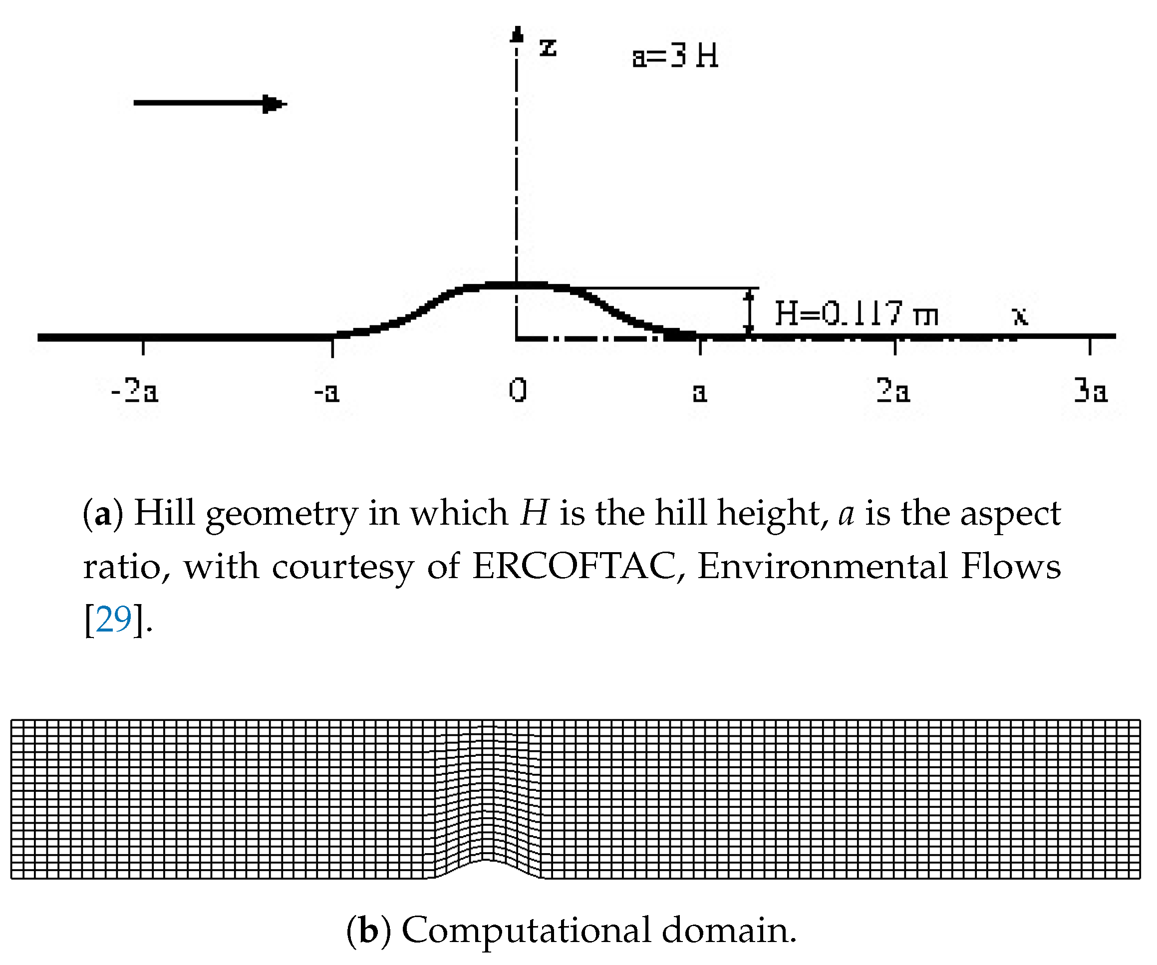
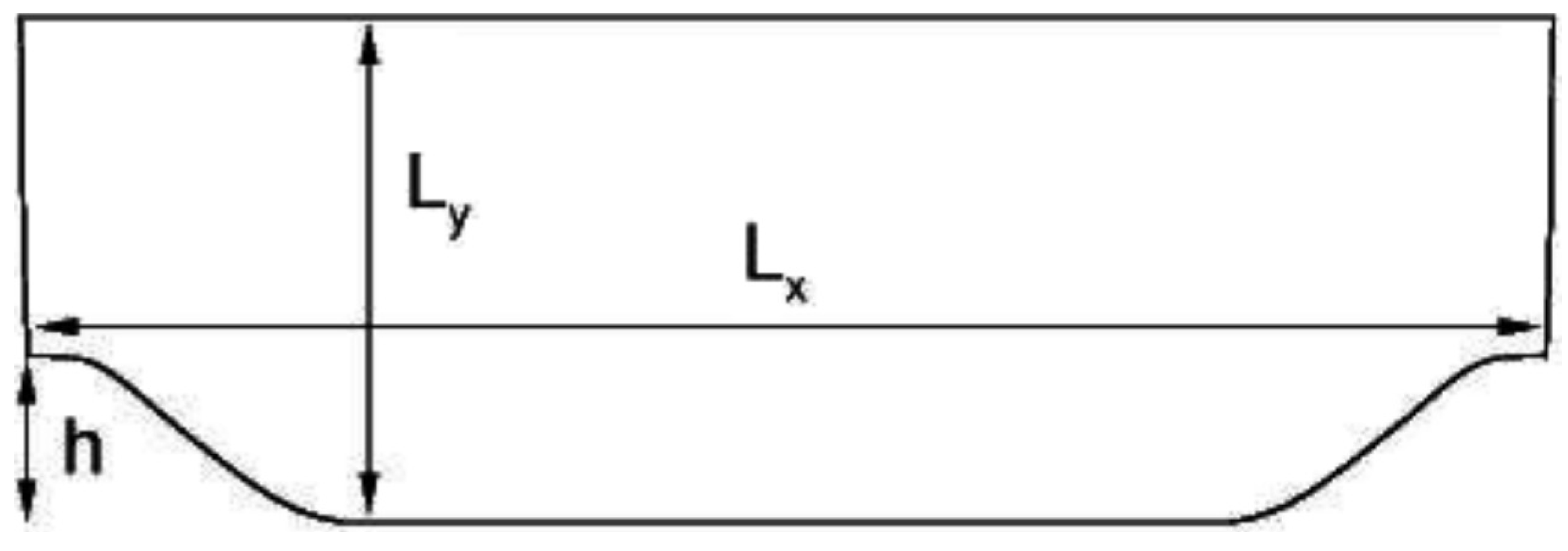
The geometry and boundary conditions are collected from ERCOFTAC classic database, environmental flows area, case 69 (http://ERCOFTAC/case69) [29]. The hill height is m and the amplitude of the hill is (Figure 1a). The wind tunnel experiments were carried out by Khurshudyan et al. [30]. A wall-resolved LES of turbulent boundary layer over a 2D hill was also performed by Chaudhari et al. [31] and Chaudhari [32] for two different aspect ratios and . Since they faced difficulty in validating the reattachment point for the aspect ratio of with the experiment, this case was specifically chosen for this study as a challenging problem.
A domain dimension with streamwise length , height and width (in spanwise direction) is considered where m.
The boundary conditions are given as follows: At the inlet, inflow is obtained from simulation of a periodic open channel flow with the same cross-sectional grid resolution; a cross-sectional plane was considered to collect the instantaneous data at each time step after the channel flow reached a steady state and the collected data was used as inflow for the flow simulation over the hill. The roughness characteristic height of the wall for this case is mm, shear velocity m/s and the Reynolds number based on shear velocity is ; at the outlet, radiative boundary conditions were given; at the upper boundary the free slip condition is imposed; periodic conditions are applied along the spanwise direction. The dynamic SGS model wis employed for simulations with body fitted grid, with the constant obtained from spanwise averaging; simulations were run with a fixed Courant number equal to .
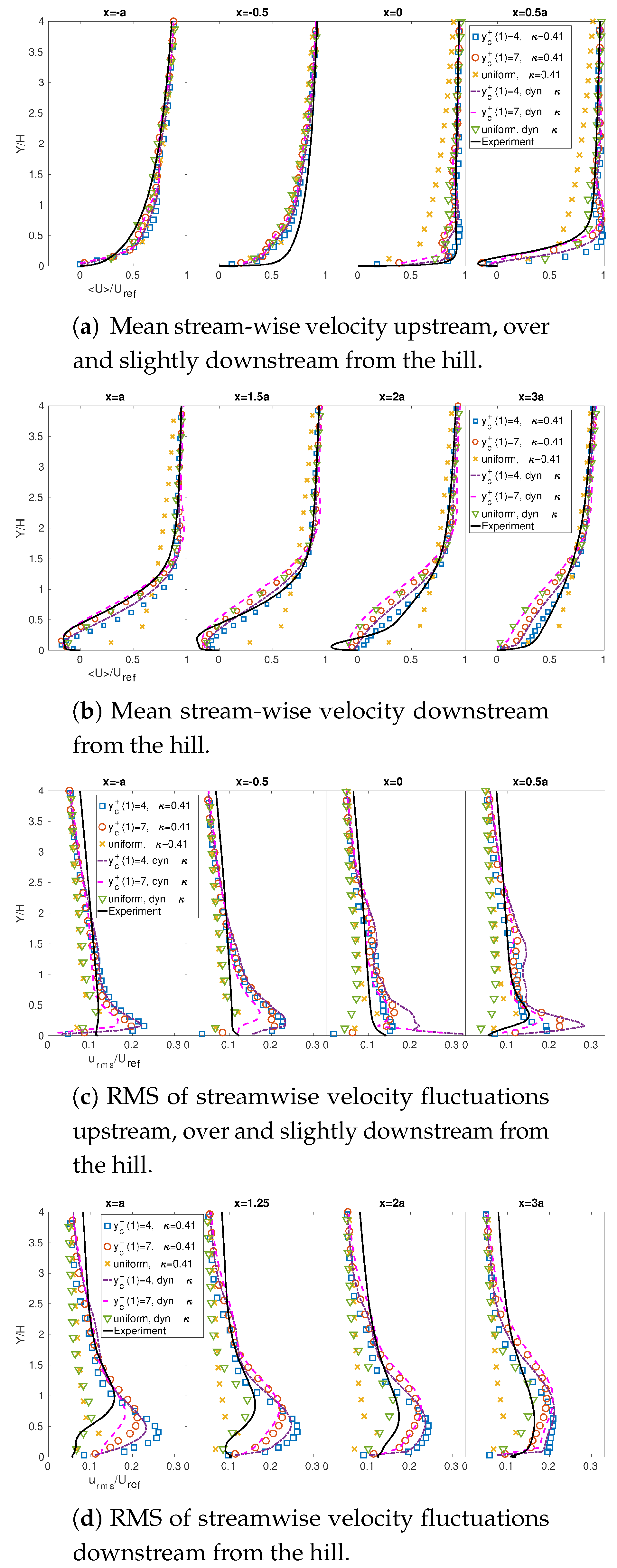
The results of this simulation, which was initially performed using cells in streamwise, wall normal and spanwise directions, respectively, show that the wall layer model described in Section 3, with a fixed value of the von Kármán constant, is not able to capture flow separation when a uniform grid is employed (where ). Conversely, stretching the grid to set the first computational node off the wall inside the viscous layer allows obtaining flow separation. Figure 2 shows a comparison between the experiment by Khurshudyan et al. [30] and three simulations: The case with uniform grid, and two cases with stretched grids in which the first centroids are at and , respectively. All the grids share the same number of grid cells and the resolution in streamwise and spanwise directions, while the two grids are stretched vertically using the Vinokur approach [33] to have the largest cells at the top of the domain with . The free surface velocity is used as to normalize the velocity plots.
For the cases with fixed value of , the starting point of flow separation is at using the stretched grids; the reattachment point is predicted well in these cases. This test reveals that the resolutions in streamwise and spanwise directions are sufficient to capture boundary layer separation. Overall, separation is predicted with a grid that for the vertical resolution near the wall resembles that of a wall-resolving LES. This is opposite the expectations from a wall layer model, which is supposed to work well with a poor resolution in the wall region.
The improved model which makes use of the dynamic evaluation of the von Kármán constant is tested on the uniform mesh. In this case separation is captured; at the first centroid is too far from the wall to capture the starting point of separation, while at the other locations, separation is predicted correctly as well as boundary layer reattachment.
Applying the dynamic evaluation of in the case of the stretched grids reveals that in the case with the mean velocity profile at demonstrates a better acceleration at the first centroid compared to the case with a fixed value of ; moreover, at , which is the starting point of separation, the negative velocity displays a larger magnitude at the few cells above the wall, which is closer to the experimental values, while a bit farther from the wall, the case with constant is in a better agreement with the experiment. In the separation region and even after reattachment, the mean velocity at the near-wall centroid is smaller than using the fixed value of , and the reattachment point is predicted correctly for . The case with demonstrates higher velocity at the near-wall computational node using dynamic in the beginning of separation (), while at and beyond, the velocity gets smaller than the fixed , and the reattachment point is delayed.
The root mean square (RMS) of streamwise velocity fluctuations exhibits an overestimation close to the wall for stretched grids using both fixed and dynamic , while the uniform grid with dynamic slightly underestimates this quantity in most of the regions. This overestimation is due to the fact that the equilibrium stress model for the rough surface computes the shear velocity and wall shear stress from the logarithmic law (Equation (12)), while the near-wall computational nodes in the stretched grids are located inside or near the viscous sub-layer.
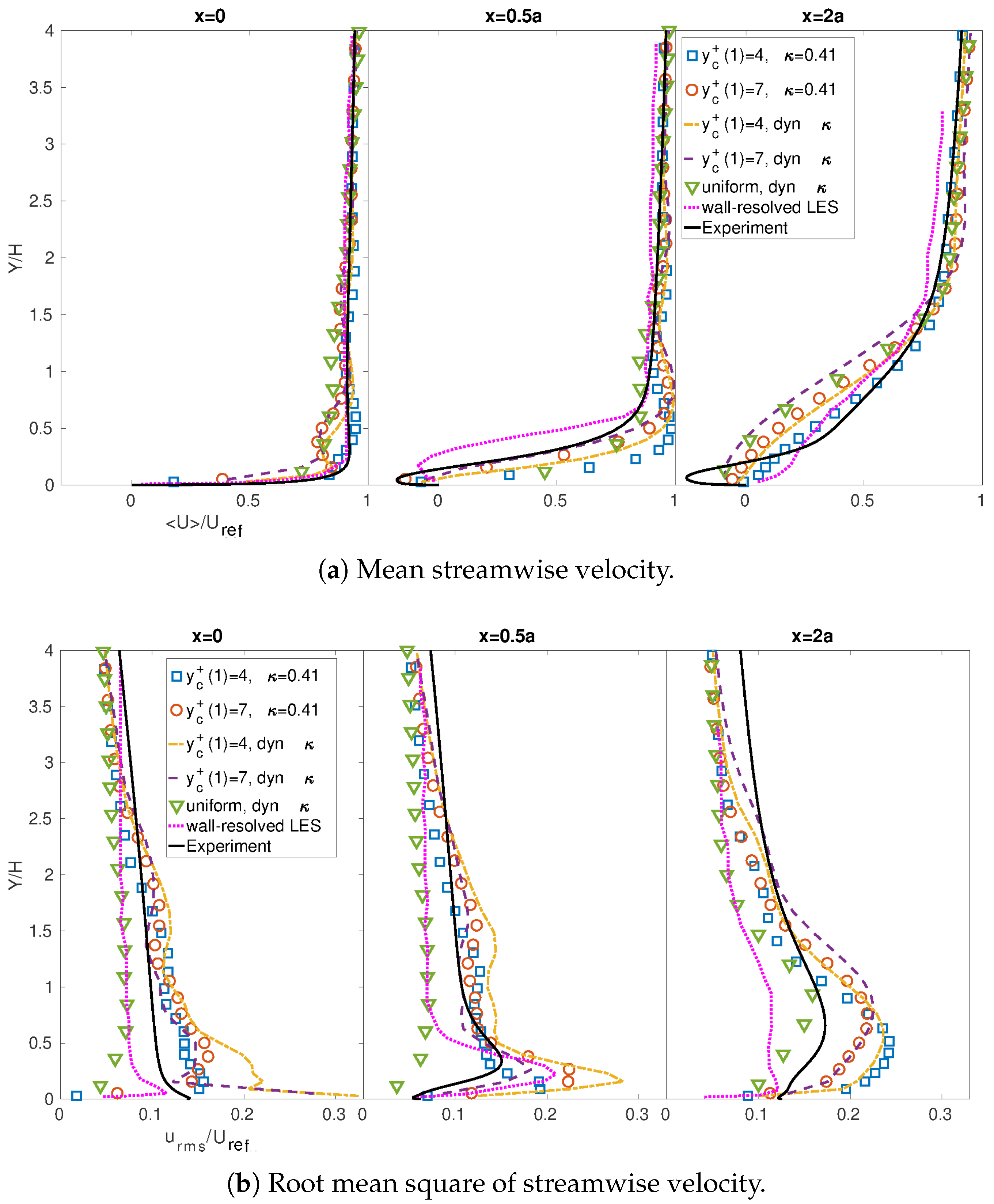
Figure 3 contains mean velocity profiles related to the present simulations, the wall-resolved LES by Chaudhari et al. [31] and the experiment by [30] at three critical locations: The hill crest, the starting point of separation and just beyond the reattachment point. For the wall-resolved LES case, the data were obtained by extraction of significant points from their plots. The mean velocity profile shows that at the top of the hill, the flow acceleration for wall-resolved LES agrees well with the experiment. Moreover, the point of separation is captured well, but the flow experiences an early reattachment at .
The wall-resolved LES underestimates root mean square of streamwise velocity fluctuations except at the start of separation close to the wall, as depicted in Figure 3b.
Figure 3a shows that, overall, the present results exhibit a reasonable accuracy, also in view of the grid herein employed. It is to be noted that the reference wall-resolved LES by Chaudhari et al. [31] with numerical grids (48 times more expensive than the current wall layer model simulation) had an early prediction of reattachment point, while in this simulation there is a better agreement of the reattachment point with the experiment.
Successively, a different grid resolution was applied in the vertical direction ( cells in streamwise, wall normal and spanwise directions, respectively) on the same geometry with the same boundary conditions. The domain grid is shown in Figure 1b, with the first computational node situated in the logarithmic region at .
The simulations were carried out as follows. First, an open channel flow at based on the friction velocity and the channel height was simulated, with a grid resolution of cells in streamwise, wall normal and spanwise directions, respectively. Before the simulation, a test was carried out to compute the dynamic (Smagorinsky) model constant and also of Equation (13) applying a plane average approach, and using as a target value of the von Kármán constant . Thereafter, in another attempt, spanwise averaging of the numerator and denominator of Equation (13) with and also the dynamic model constant was performed. Note that must be positive since it is used in the denominator to calculate friction velocity and strain rate tensor (see Section 3). Setting the minimum value of avoided unrealistic values of velocity due to the near-zero or negative value of . Moreover, larger threshold values were tested to check the sensitivity to this lower bound; the analysis showed that it does not affect the results, hence the method is robust from this aspect.
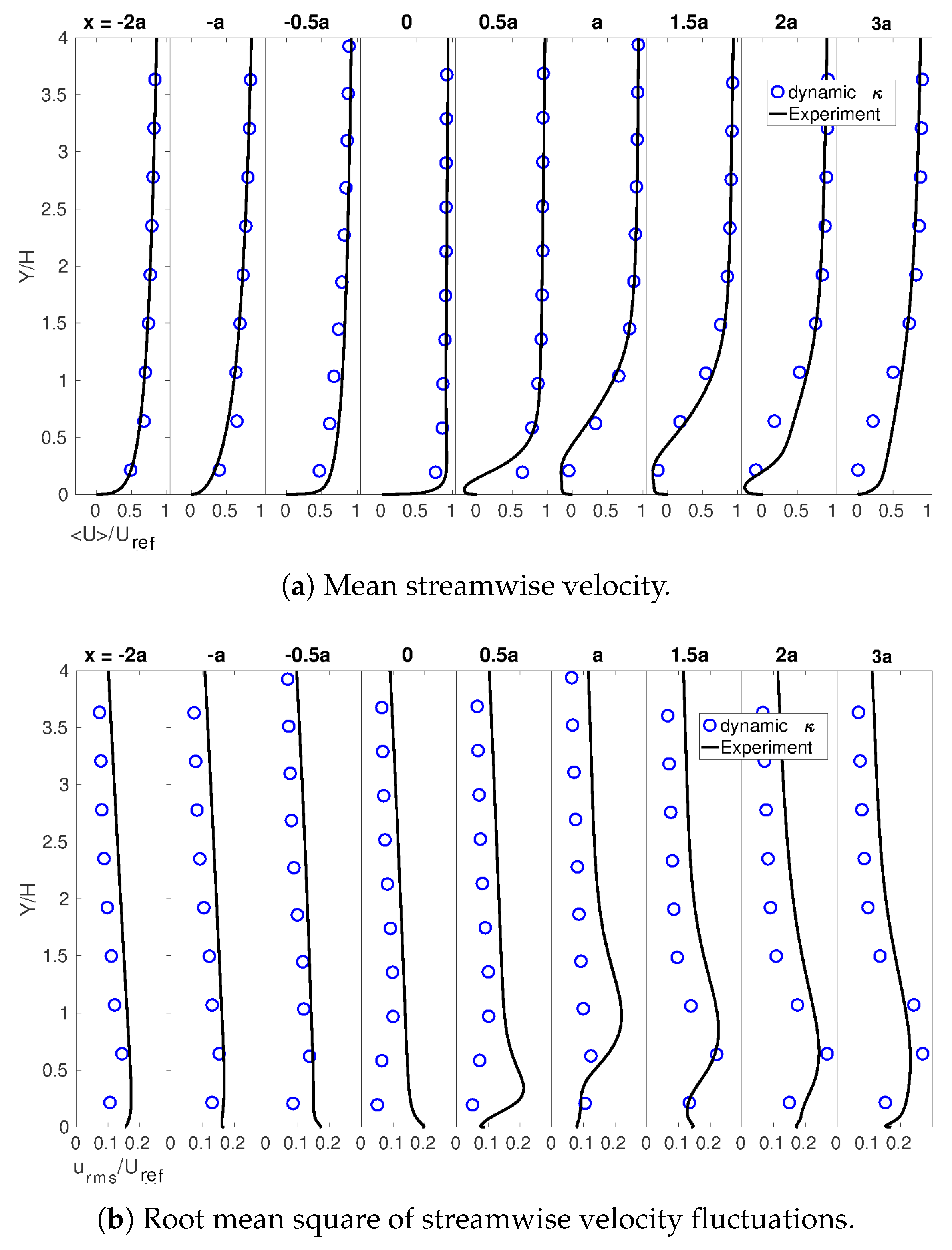
Figure 4a shows time- and spanwise-averaged velocity profiles at different positions along the streamwise direction. As expected (Figure 4a), the current resolution is too coarse, since the first computational node is out of the separation region; this explains the absence of separation at . However, separation occurs at which has a delay with respect to both the wall-resolved LES and the experiment, and reattachment is obtained at which is closer to the experiment, while the wall-resolved LES exhibits an earlier reattachment.
Figure 4b shows the root mean square of streamwise velocity fluctuations. Generally there is an underestimation of the velocity fluctuations especially right before and at the starting point of the separation region. Chaudhari et al. [31] also underestimated the RMS of the streamwise velocity fluctuations uphill, and overestimated it in the separation region.
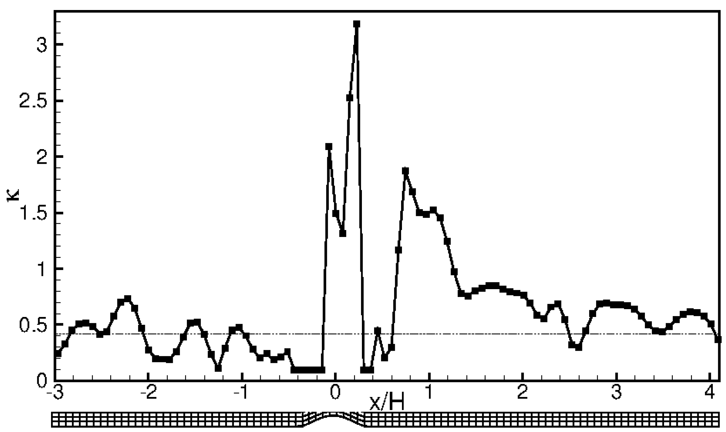
As was discussed in the previous section, the use of dynamic in this method is different than in Cabot and Moin [8]. To understand this better, instantaneous values of the dynamic along x for the flow over the single hill of this simulation in Figure 5. Since is in the numerator to calculate the shear velocity and wall shear stress (), on top of the hill, there is an increase of , which gives a better acceleration rather than the standard log law (). Then, at the starting point of separation, reduces and therefore the wall shear stress goes close to zero. Thereafter, inside the separation region, at most of the spots is large, leading to a negative value of the wall shear stress with a larger magnitude, and finally it goes close to 0.41 after reattachment. In this way, the equilibrium stress model is applicable on separated flows.
4. Wall Layer Model for Immersed Boundary Methodology (IBM)
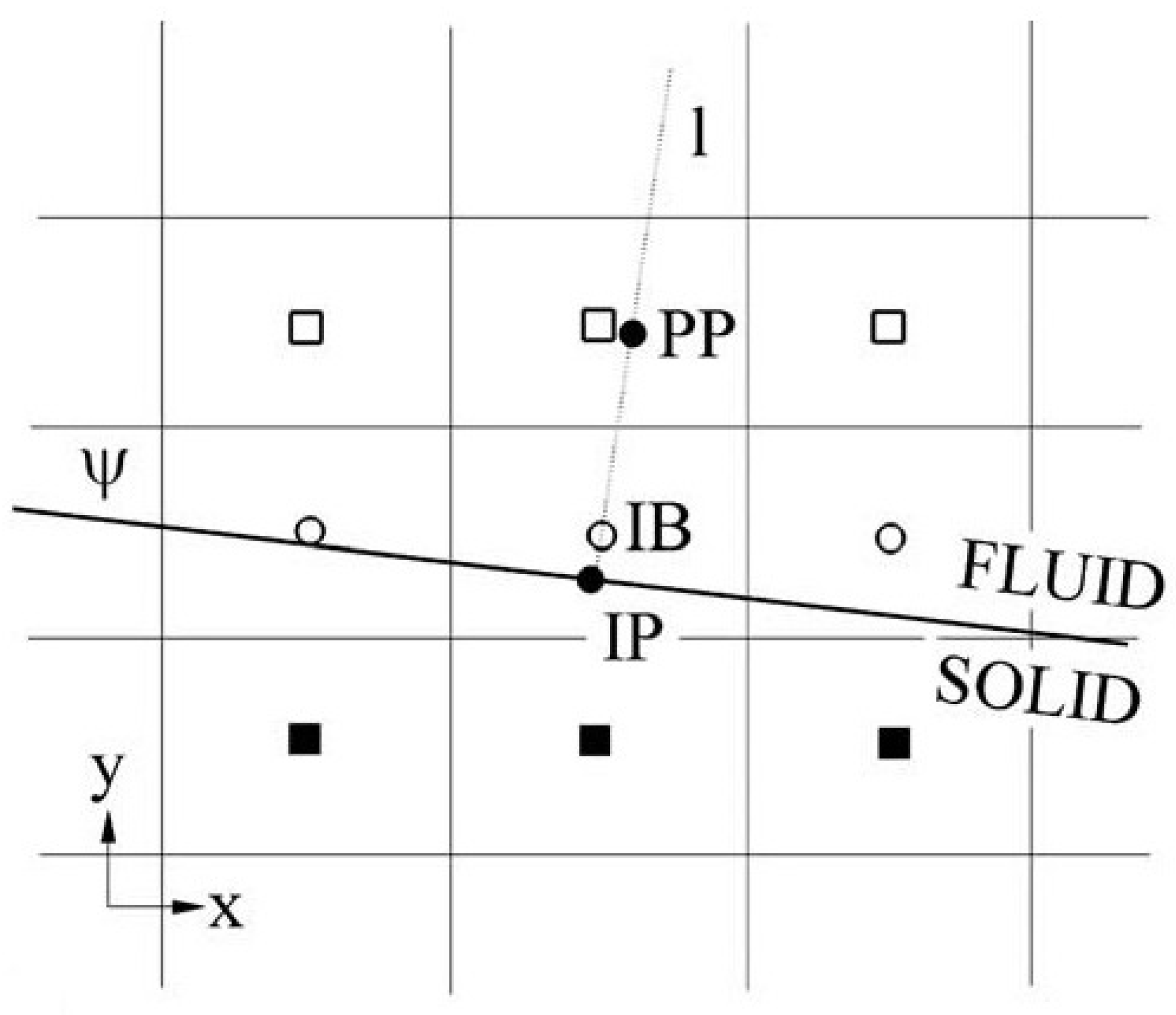
This part of the work takes advantage of the model developed in Roman et al. [34]. The velocity reconstruction method is briefly recalled here. With reference to Figure 6, the velocity at the projection point (PP) is interpolated from velocities at its surrounding points (empty square points in Figure 6). Then, shear velocity at the PP point is computed. Finally, based on the distance of the first centroid off-the-wall, i.e., the IB node, from wall in wall units, the velocity at the IB node is calculated using the law of the wall:
Considering that the velocity is known at the PP point, a parabolic interpolation is carried out to compute the wall normal velocity at the IB node:
A reconstruction of shear stress at the cell face is also done using a RANS-like eddy viscosity. The eddy viscosity at the IB nodes is calculated analytically from mixing the length theory from the equation
where is the von Kármán constant, and is an intensification coefficient to be determined such that the Reynolds shear stress is a fraction of the wall shear stress near the wall (where is set). Consequently, this coefficient can be written as:
where the index F denotes a quantity calculated at the cell face, is the distance between the cell face and the immersed surface. A more detailed description can be found in Roman et al. [34] and Roman [35]. This wall layer model is very economic since the velocity is just interpolated from the projection point PP, and works well in attached flows using a very coarse grid [34]. Since the interpolation is based on the logarithmic law, and the velocity direction at the IB node always follows the velocity at the PP, this method has a drawback in separated flows even setting the IB node inside the viscous layer.
Simulation of the flow over the hill, applying Cartesian and curvilinear grids, using the Roman et al. [34] model in its original formulation, does not allow to obtain acceptable results, since the flow does not separate even with increasing resolution close to the immersed boundary and with setting the of the IB node inside the viscous layer [28]. Here, first the Roman et al. [34] model on a standard open channel flow is re-analysed and successively the flow over the hill is investigated.
4.1. Calibration of the Wall Layer Model with IBM
In order to check the accuracy of the current IBM, an open channel is considered with a resolution of cells in the streamwise, wall normal and spanwise directions, respectively, and a dimension of in which is the height of the open channels. The lower wall is reproduced with immersed boundaries and the simulation is carried out imposing a non-dimensional driving pressure gradient (). The friction Reynolds number is , giving the IB node as located at .
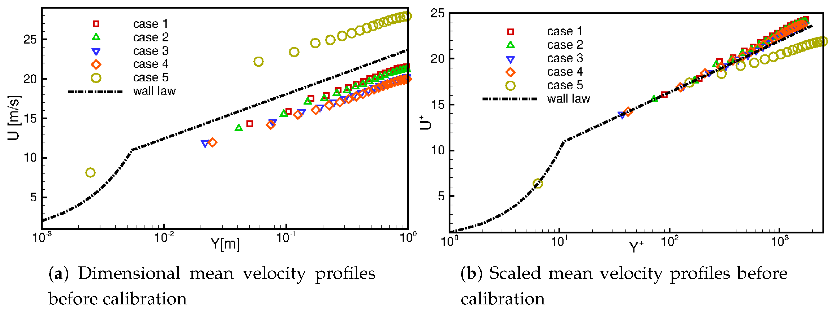
The velocity profile scaled with the friction velocity collapses over the theoretical line as has already been shown in Roman et al. [34]. However, considering the non-scaled averaged velocity, the method underestimates the velocity compared to the logarithmic law at the same rate as the shear velocity, thus demonstrating a loss of momentum. In particular, the wall shear stress is underestimated by approximately in the simulation. This has to be attributed to the current implementation of IBs, which does not conserve momentum perfectly. This is a common issue in a number of IB methodologies, although more recent implementations appear more conservative (Kim et al. [36], Meyer et al. [37] and Rapaka and Sarkar [38]).
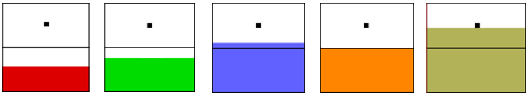
After this observation, several cases of open channel geometries are created sharing the same dimension and resolution; the only difference stands in the fact that the immersed boundary surface was moved slightly to check whether the position of the IB node affects the results. Five cases are considered: Cases 1 to 4 in which the IB node was located in the logarithmic region, and case 5 in which it was in the viscous layer. The positions of the immersed boundary for the five cases are displayed in Figure 7 and details are given in Table 1. Simulations are hence carried out for all cases at , with the same boundary conditions as the original case. The results show an underestimation of friction velocity for cases 1 to 4 in which the IB node is set in the logarithmic region, and an overestimation of shear velocity for case 1 which has the IB node in the viscous layer (see Table 1), indicating that the IBM of Roman et al. [34] is sensitive to the position of the immersed surface with respect to the grid line, and it is geometry dependent. Figure 8a displays a non-scaled mean velocity profile for all cases compared to the theoretical velocity based on the law of the wall.
Apart from the shear velocity deviation, the non-dimensional velocity profile compared well with the wall law for the first four cases (Figure 8b). A calibration of the IBM is carried out to avoid momentum loss. For this purpose, the coefficient which is used to calculate eddy viscosity at the IB nodes () in Equation (16) is varied to reach the target value of the wall stress.
Table 2 shows the optimal coefficients and friction velocities obtained after running the simulations for all five cases. Further, it has been verified that changes in the coefficients by produced very small variations in the shear velocity, thus showing the robustness of the method.
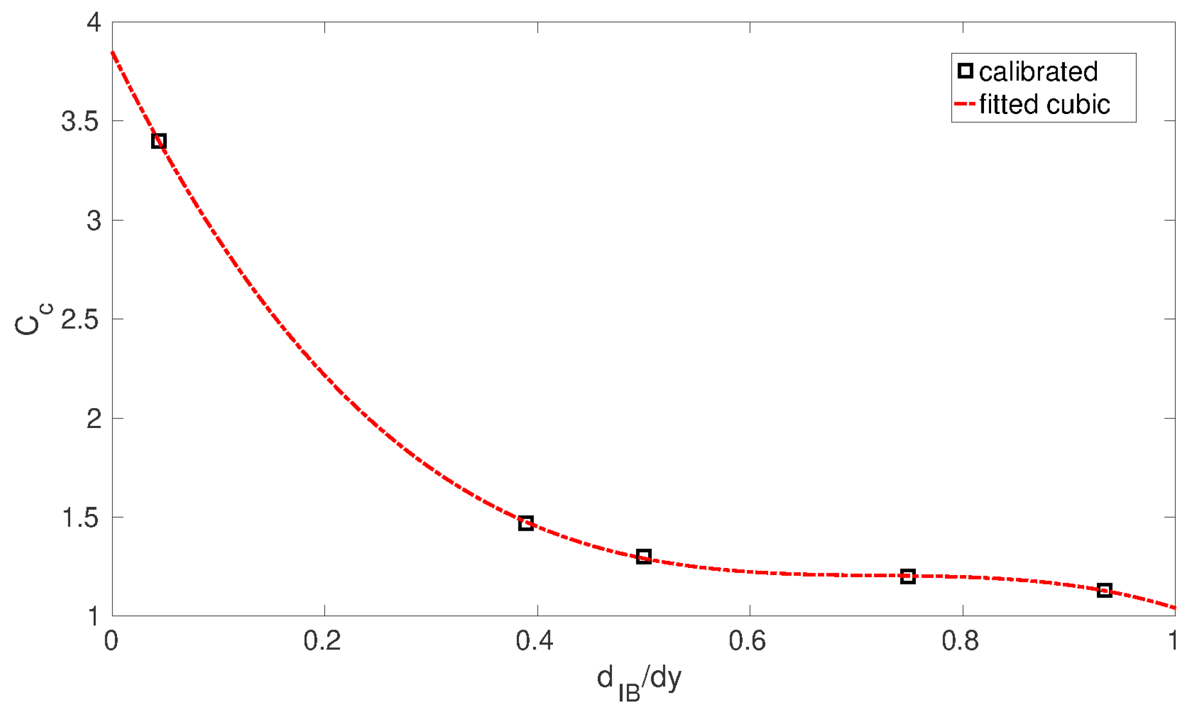
The simulations are then repeated at to check the accuracy of the calibration; it appeared insensitive to variations in the Reynolds number [28]. The coefficient can be written as a function of the non-dimensional distance from the wall (), which is within the interval of 0–1. As it can be seen in Figure 9, a cubic law can be fitted to the numerical points is written below.
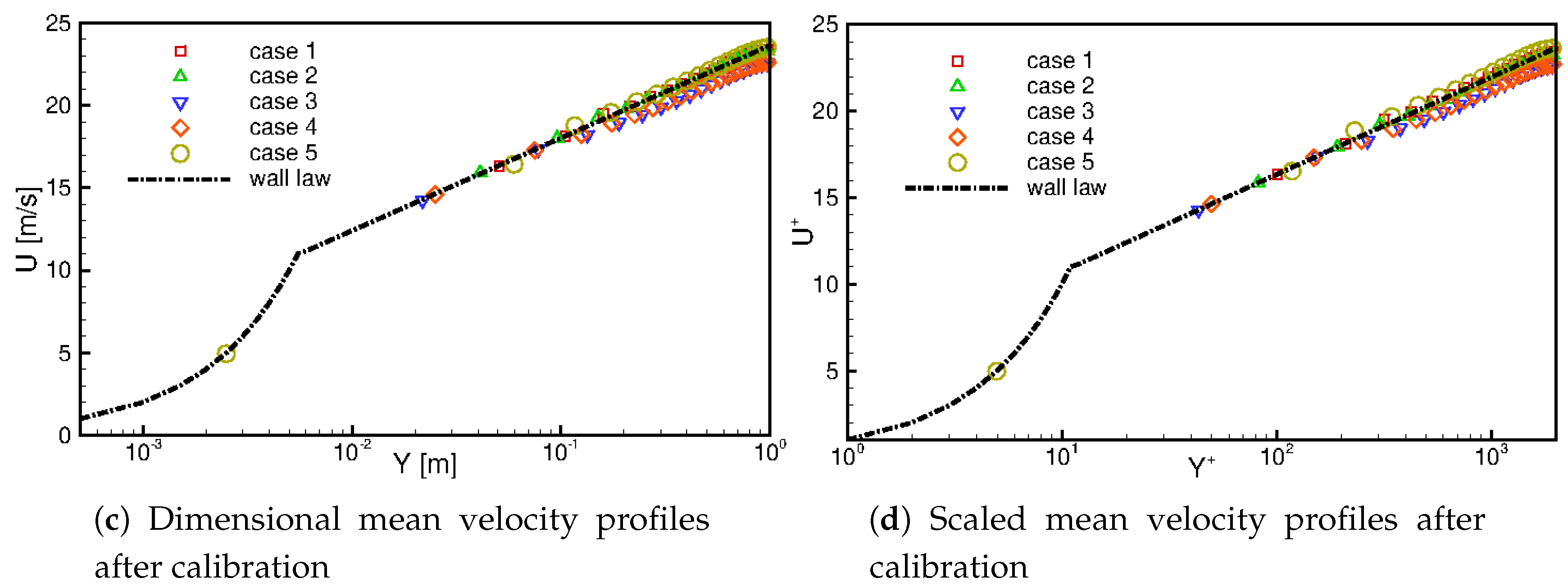
The dimensional and non-dimensional mean velocity profiles after calibration for all the cases are shown in Figure 8c,d, respectively. All cases are non-dimensionalized with shear velocity obtained from the mean velocity at the IB nodes based on the law of the wall. An improvement can be observed after calibration, especially for case 5 in which the IB node is located close to the immersed boundary. Finally the RANS-like eddy viscosity at the IB nodes can be calculated from the calibrated coefficient , which is obtained from the cubic fitting:
Calibration of the coefficient allows to improve the prediction of the wall shear stress, hence, the velocity profile. The results of the simulations for all cases show that the mean velocity and root mean square of velocity fluctuations are in good agreement with the law of the wall and also the DNS of plane channel flow of Hoyas and Jimenez [39] for a channel at [28]. Only for cases 3 and 4 in which IB nodes are at the beginning of the log-region () is there a deviation of the mean velocity profile. However, this is a case that can be hardly encountered in real-scale flows, characterized by very high values of . It is important to point out that calibration may not be necessary in the presence of IB methodologies strictly conservative for momentum.
While the wall layer model predicts the velocity profile well, it underestimates the wall normal velocity fluctuations. Thus, random fluctuations near the wall are added to improve the model. In hybrid LES/RANS and DES, stochastic forcing is needed to reduce the effect of excessive damping coming from the RANS eddy viscosity [11,12]. In the present model, stochastic forcing is more likely required because of the grid coarseness, which is, however, a standard in simulations for engineering purposes.
Taylor and Sarkar [40] used random stochastic forcing in the wall normal direction after finding that the near-wall model (NWM) LES with the dynamic eddy viscosity model (DEVM) underrated vertical velocity fluctuations in their body fitted plane-channel-flow simulation.
This forcing term was applied to the right-hand side of the momentum equation in the wall normal direction to increase velocity fluctuations in this direction and control the Reynolds stress in order to allow it to fit the logarithmic velocity profile. This term is written as:
where R is a random number between 0 and 1, and is an amplitude function. At each time step, the latter can be obtained from summation of the amplitude at the previous iteration, and another term including the error function:
where the error function is the difference between the resolved shear stress and the theoretical value based on the logarithmic law:
where is a relaxation time. This approach is correct if the first computational node is in the logarithmic region since in Equation (22) the error is established upon , which is the theoretical resolved shear stress based on the logarithmic law. However, this is not a serious issue, since the model is designed to work for high number flows. Finally, the sign of the function is computed to reduce the correlation between streamwise and vertical velocity fluctuations ( and ) if the error is positive, and to enhance this correlation if the error is negative:
where is the velocity in the direction of the mean wall shear stress.
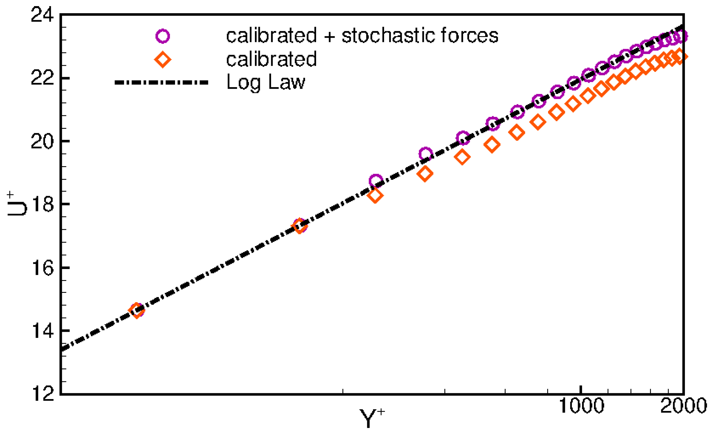
The stochastic random force in case 4 is imposed instantaneously at every iteration of the simulation. Since the IB node is located in the logarithmic region, the horizontal velocity is interpolated based on the logarithmic law from the projection point PP; adding this force to the first two nodes does not improve the velocity profile. Considering one more point to impose the forcing term on, it makes the deviation from the log law disappear (Figure 10).
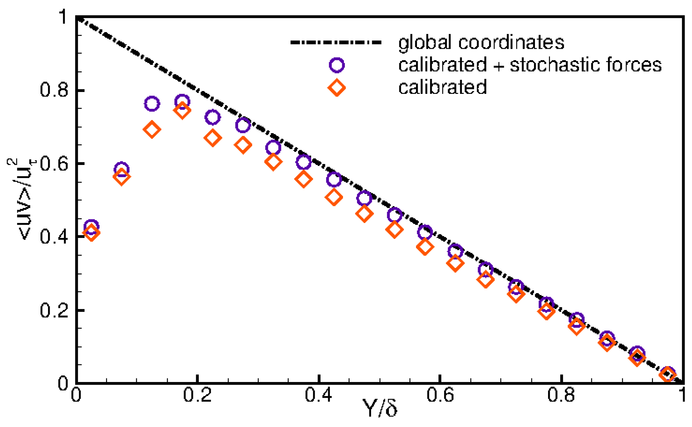
This happens because the stochastic forcing allows to obtain a more accurate prediction of the resolved Reynolds shear stress (associated to the resolved velocity fluctuations) as can be seen in Figure 11.
The relaxation time plays an important role in the simulation. It has to be large enough to let the flow adapt itself to the force. On the other hand, if the relaxation time is too large the effect of force is diluted. In the present simulations, gave the best results. Values larger than increased the velocity continuously since the flow did not have time to adjust itself to the force; values smaller than displayed a very small improvement in velocity profile.
This method works very well when the IB node is located in the logarithmic region and in attached flows since a logarithmic law for the velocity profile is expected. However, in the present form, it is not able to predict massive separation.
Steady two-dimensional separation is known to be related to the sign of the streamwise pressure gradient. After neglecting advective terms, the boundary layer equation in the streamwise direction simplifies as:
Considering the flow over a curved surface, a negative streamwise pressure gradient develops upward, associated to an acceleration of the flow. Thereafter, the change of curvature makes the pressure gradient become unfavourable, and from the continuity equation it contributes to an enhancement of the boundary layer thickness. Hence the second derivative of velocity is positive and therefore there is a change of sign of the velocity curvature inside the boundary layer. At a point called inflection, the second derivative of streamwise velocity becomes zero; . If the unfavourable pressure gradient is strong enough, the flow next to the wall changes direction giving rise to a recirculation region. As already noted, in this method the velocity at the IB node is calculated from the friction velocity at the projection point. This means that is always in the same direction of , and the flow is not allowed to separate, since the above-described physical mechanism is not accounted for. For this reason, the method of calculation of the velocity at the IB point is modified as follows. The boundary layer equation close to the wall, after neglecting advective terms is:
Using the central difference scheme (CDS) in order to discretize the second derivative of velocity for a non-uniform grid (Ferziger and Peric [41]) considering PP, IB and IP nodes, it can be written as:
in which is the distance between IB and PP points. Finally the streamwise tangential velocity at the IB node can be written as a function of the tangential pressure gradient instead of the friction velocity;
where the eddy viscosity is also the calibrated value obtained from Equation (19).
Using a coefficient (C) of the order of inside the second term containing the pressure gradient at the IB avoids problems in regions characterized by the presence of large values of the pressure gradient with small values of turbulent eddy viscosity. Many simulations have been carried out to find out the best criterion for using this new scheme. Finally, applying Equation (27) under the following conditions:
gave the best results for simulating separated flows. The two criteria physically mean that the new scheme to calculate tangential velocity at the IB is used if the tangential pressure gradient at the IB is unfavourable, and the distance of the IB node from the immersed boundary is such that the velocity point does not belong to the log region of the velocity profile.
4.2. Flow Simulation over a Single Hill Using IBM
This new model is applied for simulation of the flow over a two-dimensional hill. First an open channel is constructed in which the immersed boundary is set as the lower wall. After the periodic open channel flow reached a steady state, instantaneous data are collected from a cross sectional plane at different time steps. Then the bottom of the domain including the hill shape is created as the immersed boundary, and the data that are obtained from the plane channel flow are used as inflow for the flow simulation over the hill.
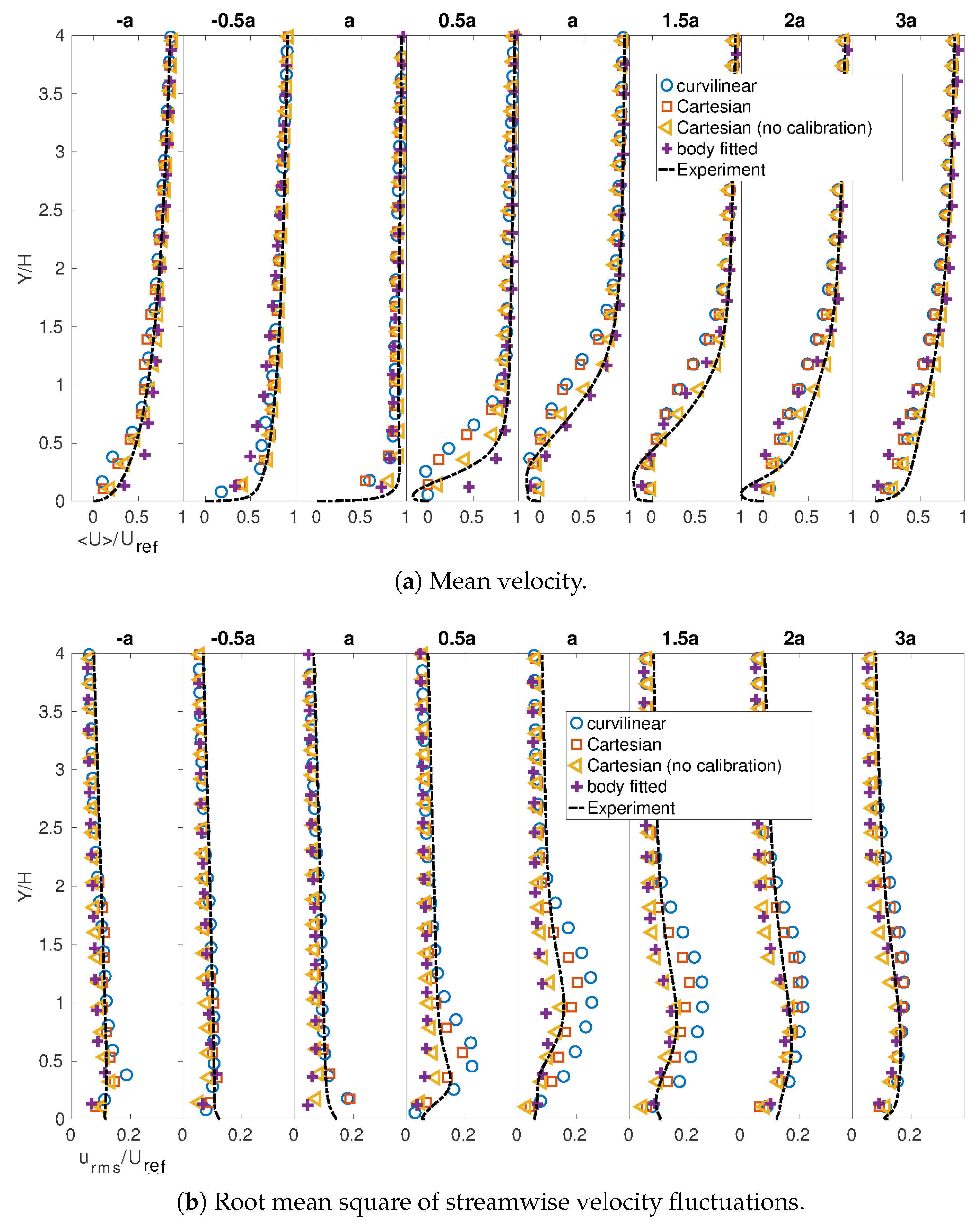
The simulation is performed using two different grids (Cartesian and curvilinear) at . Applying the new scheme, it is feasible to capture separation in the simulation with a grid resolution of cells in the streamwise, wall normal and spanwise directions, respectively. With this resolution, the IB node upward and downward from the hill is located at . The mean velocity profiles for both grids are compared with the body fitted approach and the experiment by Khurshudyan et al. [30] as shown in Figure 12a. In the simulation for both grids, the starting point of separation is predicted well at . The reattachment points for both cases are anticipated before ; therefore, at the mean velocities are positive, although very small close to the immersed boundary.
In addition, for the Cartesian grid a simulation without calibration is performed to check the effect of eddy viscosity calibration on flow separation; as it can be observed in Figure 12a, the case without calibration is not able to capture the starting point of separation properly, and in general it underestimates separation.
The root mean square of streamwise velocity fluctuations of the present simulations (Figure 12b) are in a good agreement with the experimental data. While there is an overestimation of fluctuations beyond the starting point of separation, the behavior of this quantity is similar to that of the experiment. Comparing the results of the present model with the one developed for the body fitted grid, it appears that the present IBM anticipates the starting point of separation in better agreement with the wall-resolved LES and the experiment, while the prediction of the reattachment point is similar to the wall-resolved LES, earlier than in the body fitted approach and the experiment. The present IBM gives more energetic velocity fluctuations than the body fitted approach. Moreover, comparing this result with the wall-resolved LES by Chaudhari et al. [31], it can be stated that the mean velocity profile has similar behavior: Predicting the starting point of separation well, and undergoing an early reattachment. The RMS of streamwise velocity fluctuations is also similar to the wall-resolved LES; depicting marginal underestimation before and after the separation region especially far from the wall, and an overestimation inside the separation region near the wall.
4.3. Flow Simulation over 2D Periodic Hills
Finally, the new scheme is tested on flow over two-dimensional periodic hills with polynomial shape (Almeida et al. [42]). It is Case 81 of the ERCOFTAC classic database (http://ERCOFTAC/cases/case81) [43]. The shape of the domain is shown in Figure 13.
The edges of the domain are at the top of the hill. The hill height is mm, and the crests of the two successive hills are separated by . The height of the channel is equal to , and the channel width is . The reference for comparing the results are the mean velocity and RMS of the velocity fluctuations obtained from resolved LES by Temmerman and Leschziner [44] available in ERCOFTAC, and for separation and reattachment points, obtained from resolved LES by Fröhlich et al. [45] from the NASA Langley Research Center database (http://nasa/LES/2dhillperiodic) [46].
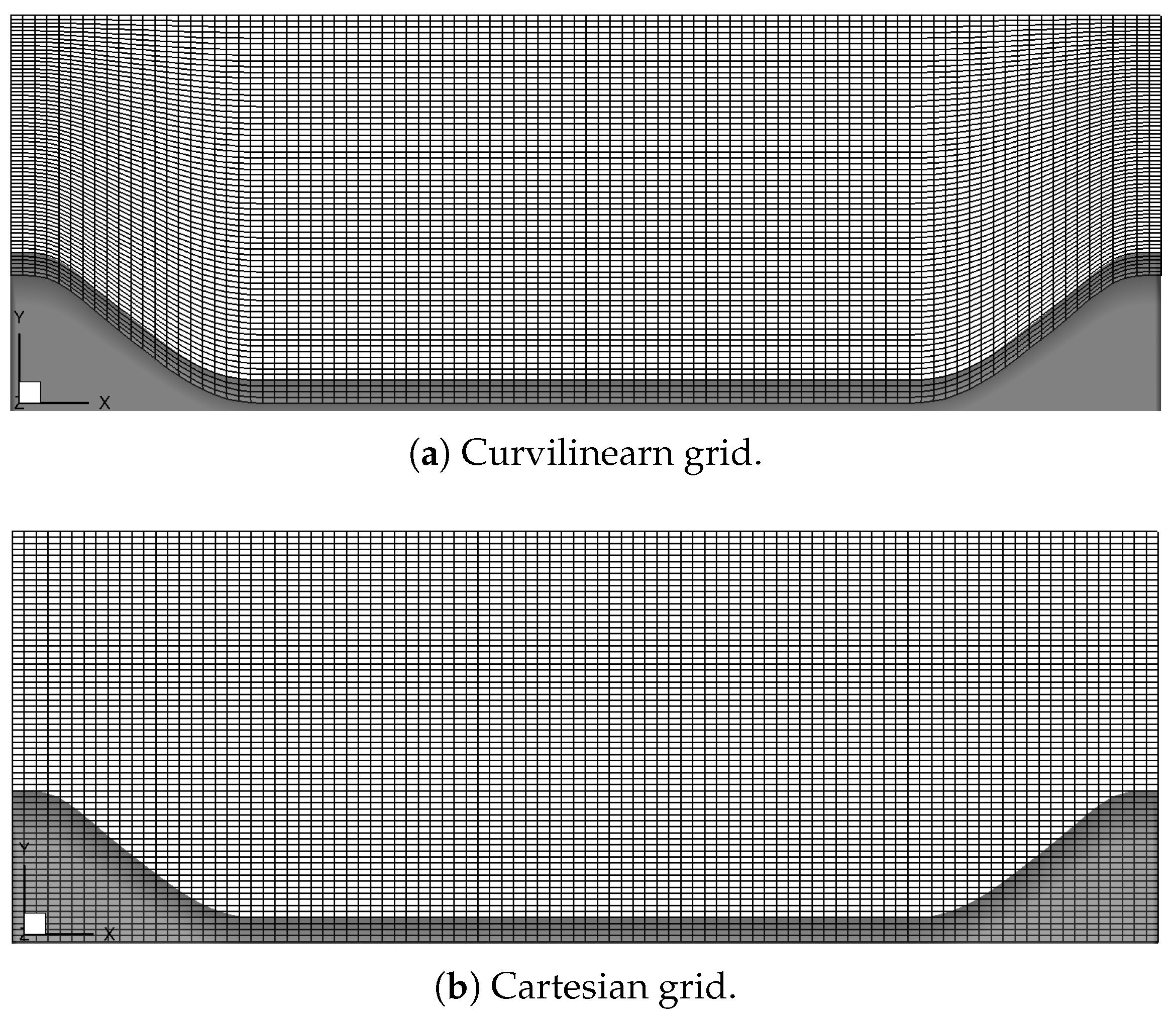
The computational domain is created in two different ways, using Cartesian and curvilinear grids, respectively (see Figure 14). The latter is shaped in such a way as to follow the hill geometry. In both cases, the bottom surface is created as an immersed boundary. The Reynolds number based on the hill height and bulk velocity on top of the first hill is equal to , where is the molecular viscosity. The flow is periodic in the x and z directions, using immersed boundary at the bottom and free-slip surface at top.
A domain with grid resolution of cells out of immersed boundary in streamwise, wall normal and spanwise directions, respectively, is constructed. This is equivalent to the coarsest grid of Chen et al. [17], who simulated flow over periodic hills using immersed boundary and applied a zonal approach (TLM); in particular, the authors used the turbulent boundary layer equations close to the immersed boundary and LES in the interior region.
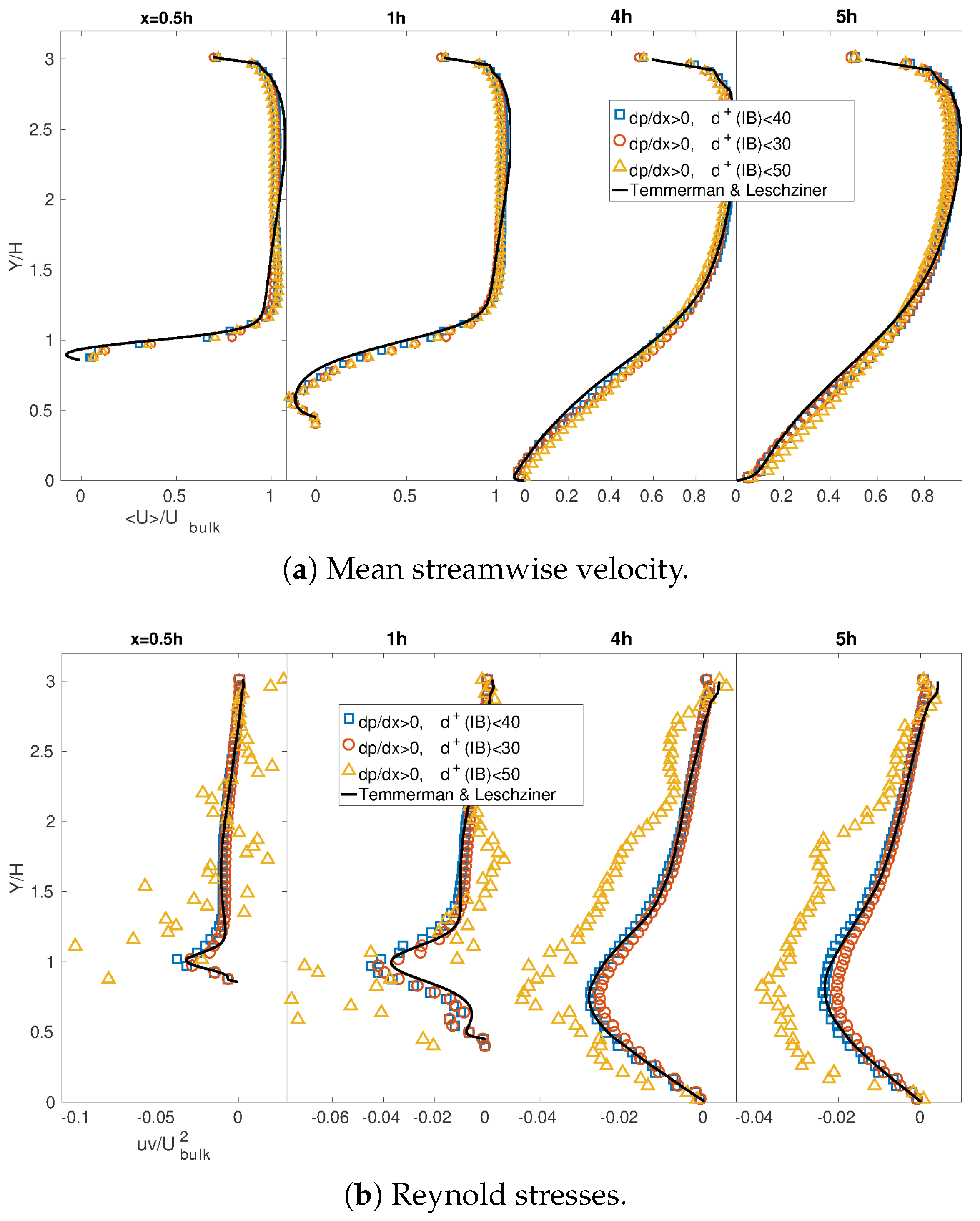
The robustness of the method to reproduce separation is tested under a large variation of the threshold values employed in Equation (29). The results of this test for the threshold in the range of 30–50 are shown in Figure 15. The mean velocity profile in Figure 15a shows that in all cases separation is captured at , but using makes the reattachment point shift back slightly with respect to the other cases and the wall-resolved LES. The mean velocity profile for is marginally closer to the resolved LES compared to (which overestimates it narrowly). In addition to the mean velocity profile, Reynolds shear stresses for demonstrates better agreement to the wall-resolved LES in the separation region and after reattachment (Figure 15b). Overall, it can be stated that the method is robust for large variations of the threshold value chosen to switch from one to the other law for the velocity at the first grid point. Large variations of this value produce marginal variations in the results.
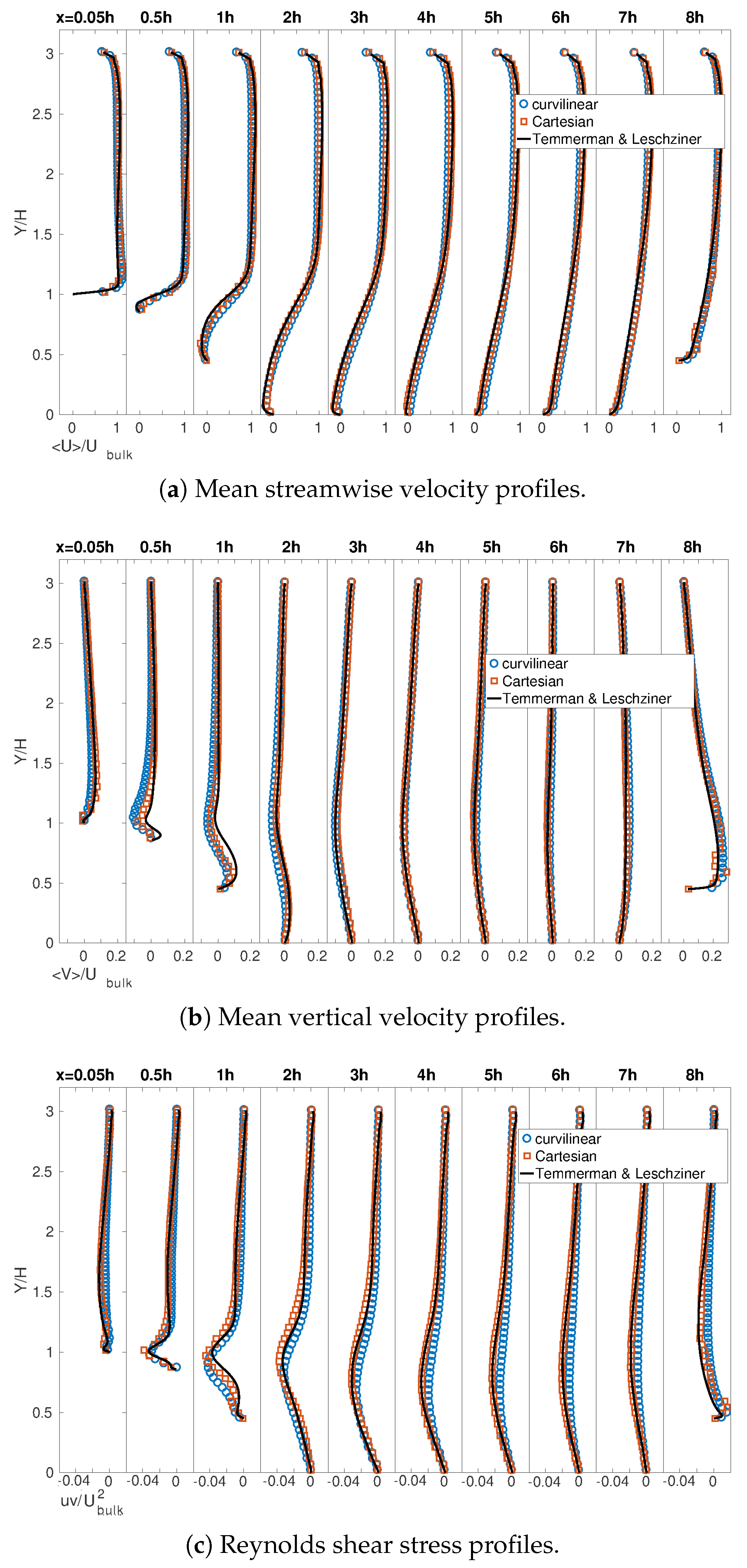
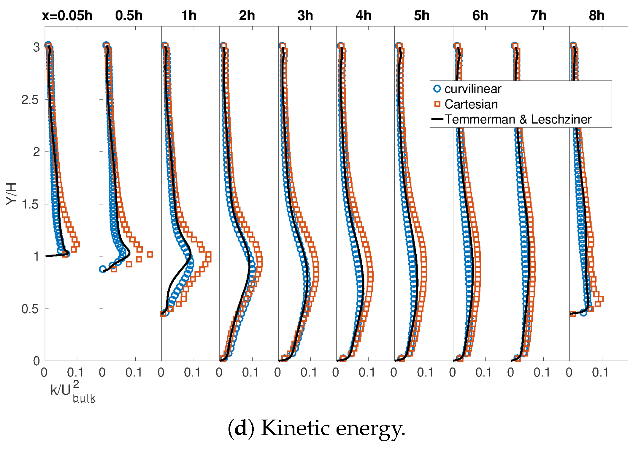
Figure 16 depicts statistics of the simulations of flow over periodic hills compared to the wall-resolved LES by Temmerman and Leschziner [44] at ten different streamwise locations. Velocities are made non-dimensional with which is the bulk velocity on the first hill crest; moreover, Reynolds stress and turbulent kinetic energy are non-dimensionalized with .
Figure 16a shows mean streamwise velocity profiles (averaged in time and the spanwise direction) at different streamwise locations. They are overall in good agreement with the wall-resolved LES by Temmerman and Leschziner [44]. While the mean velocity for the Cartesian grid at matches the profile obtained from the wall-resolved LES, the velocity is not negative at the IB node, while the curvilinear grid displays a negative velocity at the IB node in this location. Separation is captured in both Cartesian and curvilinear grid cases, and the reattachment point for the Cartesian grid is a bit earlier than the resolved LES, while the flow in the curvilinear grid reattaches earliest before .
The mean vertical velocity profiles in Figure 16b show a slight underprediction for both grids downhill, but in the other locations they matched the wall-resolved LES data.
Figure 16c displays the Reynolds shear stress for both cases (based on the resolved fluctuations). It behaves similarly to that of the resolved LES, while a marginal underestimation is observed before the end of downhill at near the immersed boundary, especially in the case with curvilinear grid.
As illustrated in Figure 16d, turbulent kinetic energy for the Cartesian grid is slightly overpredicted with respect to the wall-resolved LES, while the curvilinear grid demonstrates a closer value to the reference data. Overall, the behavior of this quantity is similar to that of the wall-resolved LES for both cases.
Table 3 displays the separation and reattachment points in the current simulation, the wall-resolved LES of Fröhlich et al. [45] and WMLES (using two-layer model) of Chen et al. [17]. In the present simulation, the boundary layer separation occurs at with the Cartesian grid and at with the curvilinear grid; in the wall-resolved LES it happens at . Therefore a delay is observed to predict the separation point. Moreover, the intensity of the recirculation bubble predicted by the optimized IBM simulations is smaller than that of the wall-resolved LES (comparing the present simulation values with the large negative values of the reference simulation). The wall-resolved LES shows the reattachment point at , while in the current simulation the boundary layer reattaches a bit earlier in both cases; the Cartesian grid predicts the reattachment point at , while the curvilinear grid anticipates it at .
Overall, the agreement of the simulation result is acceptable, considering the simplicity of the model, which does not require the solution of an additional equation in the wall layer and the number of grid points employed in the tests. Moreover, in comparison to the simulations of [17], the new wall layer model on the Cartesian grid predicts the separation point better than their case with the same resolution, and on the curvilinear grid it is even closer to the reference data than the WMLES of [17], but the reattachment point in their case is predicted closer to the reference. The other statistics obtained from the current simulation, especially the mean vertical velocity profile, are in better agreement with the wall-resolved LES than the simulations of [17].
5. Summary and Conclusions
In the present paper, a wall layer modeling for massive separation has been developed within the LES context. Two main frameworks have been considered; namely, the case where the solid wall is reproduced using a body fitted curvilinear grid and the case where the solid surface is simulated with immersed boundaries. The research aimed at developing a simple wall layer model to be used in conjunction with LES for engineering applications where the near-wall resolution is generally coarse. The starting point was the equilibrium wall layer model, which gives good results in attached flows [47]. In the case of body fitted curvilinear grids, the equilibrium wall layer model was improved using the dynamic procedure of Cabot and Moin [8] in a new fashion. The dynamic was applied on the log law without using TBLE in order to deviate the wall shear stress and the two components of strain rate tensor from the standard log law.
When the solid surface was simulated with immersed boundaries, a different strategy was accomplished. The starting point was the equilibrium wall layer model of Roman et al. [34], in which the velocity at the near-wall nodes was reconstructed from a farther point (the projection point) based on the law of the wall, and a RANS-like eddy viscosity was given at the IB node. To reconstruct the fluctuations in the wall normal direction well, especially near wall, random stochastic forcing was applied to the first three near-wall cells. Moreover, the model was complemented with a procedure designed at reproducing massive separation without the need to use zonal approaches. Specifically, after removing the advective terms from the boundary layer equation, the tangential streamwise velocity at the IB node () was obtained from the pressure gradient instead of calculating it from shear velocity at the projection point based on the law of the wall: When the pressure gradient was unfavourable and the IB node was not in the log region, the tangential velocity was obtained through a balance between the wall normal diffusion term and the streamwise pressure gradient. In some sense, this represents a simplified procedure with respect to the zonal approach where the boundary layer equation is solved within the near-wall layer. In order to check what grid topology is best suited for reproducing this kind of flow, both Cartesian and curvilinear grids were considered in conjunction with immersed boundaries.
The models were tested and validated over two two-dimensional geometries, both being well studied in the literature through physical and high-resolution LESs: First the isolated hill (case 69 of the ERCOFTAC classic database) was considered; then, the periodic hill which is case 81 of ERCOFTAC classic datasbe was considered.
The model for body fitted geometry was generally in good agreement with the reference data; the starting point of separation was delayed with respect to the wall-resolved LES and the experiment, but the reattachment point was closer to the experiment, while the wall-resolved LES displayed an early reattachment. Applying 32 and 20 cells in the vertical direction correspondent to and 60, respectively, the results were comparatively acceptable. However, decreasing the vertical resolution further would delay the starting point of separation more. The model developed for immersed boundaries gave a mean velocity profile and other statistics in acceptable agreement with the reference data on both isolated and periodic hills, also in consideration of the coarseness of the grids employed; for the isolated hill, 40 cells in the vertical direction were required to cover the hill with four cells applying the Cartesian grid, which was correspondent to ; higher resolution was not used to avoid the near-wall computational node being located in the viscous sub-layer, and lower resolution did not capture the flow separation.
For the periodic hill, 64 cells in the vertical direction gave applying the Cartesian grid. Lower resolution did not display flow separation because of an excessive under-resolution of the hill geometry.
Funding
The research has been supported by project COSMO “CFD open source per opera morta”, the grant number CUP n. J94C14000090006, law number 3865, PAR FSC 2007-2013, Friuli Venezia Giulia.
Acknowledgments
The author wholeheartedly thanks Vincenzo Armenio from Università degli Studi di Trieste, Italia, and Federico Roman from IEFLUIDS S.r.l., Università degli Studi di Trieste, Italia, for their effective collaboration to accomplish this work.
Conflicts of Interest
The author declares no conflict of interest.
References
- Piomelli, U.; Balaras, E. Wall-Layer Models For Large-Eddy Simulations. Annu. Rev. Fluid Mech. 2002, 34, 349–374. [Google Scholar] [CrossRef]
- Piomelli, U. Wall-Layer Models For Large-Eddy Simulations. Prog. Aerosp. Sci. 2008, 44, 437–446. [Google Scholar] [CrossRef]
- Bae, H.J.; Lozano-Durán, A.; Bose, S.T.; Moin, P. Dynamic slip wall model for large-eddy simulation. J. Fluid Mech. 2019, 859, 400–432. [Google Scholar] [CrossRef] [PubMed]
- Deardorff, J.W. A Numerical Study of Three-Dimensional Turbulent Channel Flow at Large Reynolds Numbers. J. Fluid Mech. 1970, 41, 453–480. [Google Scholar] [CrossRef]
- Schumann, U. Subgrid-Scale Model For Finite Difference Simulation of Turbulent Flows in Plane Channels And Annuli. J. Comput. Phys. 1975, 18, 376–404. [Google Scholar] [CrossRef]
- Balaras, E.; Benocci, C. Sub-Grid Scale Models in Finite-Difference Simulations of Complex Wall Bounded Flows; AGARD CP: Neuilly-Sur-Seine, France, 1994; Volume 551, pp. 2.1–2.5. [Google Scholar]
- Cabot, W.H. Near-Wall Models in Large-Eddy Simulations of Flow Behind a Backward-Facing Step. In Annual Research Briefs—+; Center for Turbulence Research, Stanford University: Stanford, CA, USA, 1996; pp. 199–210. [Google Scholar]
- Cabot, W.; Moin, P. Approximate Wall Boundary Conditions in The Large-Eddy Simulation of High Reynolds Number Flows. Flow. Turbul. Combust. 2000, 63, 269–291. [Google Scholar] [CrossRef]
- Spalart, P.R.; Jou, W.H.; Strelets, M.; Allmaras, S.R. Comments On The Feasibility of LES For Wings and on a Hybrid RANS/LES Approach; Advances in DNS/LES; Liu, C., Liu, Z., Eds.; Greyden Press: Columbus, OH, USA, 1997; pp. 137–148. [Google Scholar]
- Mockett, C.; Fuchs, M.; Thiele, F. Progress in DES For Wall-Modelled LES of Complex Internal Flows. Comput. Fluids 2012, 65, 44–55. [Google Scholar] [CrossRef]
- Keating, A.; Piomelli, U. A Dynamic Stochastic Forcing Method As A Wall-Layer Model For Large-Eddy Simulation. J. Turbul. 2006, 7, 1–24. [Google Scholar] [CrossRef]
- Temmerman, L.; Hadziabdic, M.; Leschziner, M.A.; Hanjalic, K. A Hybrid Two-Layer URANS-LES Approach For Large Eddy Simulation at High Reynolds Numbers. Int. J. Heat Fluid Flow 2005, 26, 173–190. [Google Scholar] [CrossRef]
- Mittal, R.; Iaccarino, G. Immersed Boundary Methods. Annu. Rev. Fluid Mech. 2005, 37, 239–261. [Google Scholar] [CrossRef]
- Roman, F.; Napoli, E.; Milici, B.; Armenio, V. An Improved Immersed Boundary Method For Curvilinear Grids. J. Comput. Fluids 2009, 38, 1510–1527. [Google Scholar] [CrossRef]
- Tessicini, F.; Iaccarino, G.; Fatica, M.; Wang, M.; Verzicco, R. Wall Modelling For Large-Eddy Simulation Using an Immersed Boundary Method. In Annual Research Briefs; NASA Ames Research Center/Stanford University Center of Turbulence Research: Stanford, CA, USA, 2005; pp. 181–187. [Google Scholar]
- Posa, A.; Balaras, E. Model-Based Near-Wall Reconstructions For Immersed-Boundary Methods. J. Theor. Comput. Fluid Dyn. 2014, 28, 473–483. [Google Scholar] [CrossRef]
- Chen, Z.L.; Hickel, S.; Devesa, A.; Berl, J.; Adams, N.A. Wall Modelling For Implicit Large-Eddy Simulation and Immersed-Interface Methods. J. Theor. Comput. Fluid Dyn. 1994, 28, 1–21. [Google Scholar]
- Roman, F.; Stipcich, G.; Armenio, V.; Inghilesi, R.; Corsini, S. Large Eddy Simulation of Mixing in Coastal Areas. J. Heat Fluid Flow 2010, 31, 327–341. [Google Scholar] [CrossRef]
- Galea, A.; Grifoll, M.; Roman, F.; Mestres, M.; Armenio, V.; Sanchez-Arcilla, A.; Mangion, L.Z. Numerical Simulation of Water Mixing And Renewals In The Barcelona Harbour Area. Environ. Fluid Mech. 2014, 14, 1405–1425. [Google Scholar] [CrossRef]
- Smagorinsky, J. General Circulation Experiments with the Primitive Equations. Mon. Weather Rev. 1963, 91, 99–164. [Google Scholar] [CrossRef]
- Lilly, D.K. The representation of small-scale turbulence in numerical simulation experiments. In Proceedings of the IBM Scientific Computing Symposium on Environmental Sciences, New York, NY, USA, 14–16 November 1967. [Google Scholar]
- Blazek, J. Computational Fluid Dynamics: Principles and Applications, 3rd ed.; Butterworth-Heinemann: Oxford, UK, 2015. [Google Scholar]
- Stocca, V. Development of a Large Eddy Simulation Model for the Study of pOllutant Dispersion in Urban Areas. Ph.D. Thesis, University of Trieste, Trieste, Italy, 2010. [Google Scholar]
- Germano, M.; Piomelli, U.; Moin, P.; Cabot, W.H. A dynamic subgrid-scale eddy viscosity model. Phys. Fluids 1991, 3, 1760–1765. [Google Scholar] [CrossRef]
- Zang, J.; Street, R.L.; Koseff, J.R. A Non-Staggered Grid, Fractional Step Method For Time-Dependent Incompressible Navier-Stokes Equations in Curvilinear Coordinates. J. Comput. Phys. 1994, 14, 459–486. [Google Scholar] [CrossRef]
- Armenio, V.; Piomelli, U. A Lagrangian Mixed Subgrid-Scale Model in Generalized Coordinates. J. Flow Turbul. Combust. 2000, 65, 51–81. [Google Scholar] [CrossRef]
- Petronio, A.; Roman, F.; Nasello, C.; Armenio, V. Large Eddy Simulation Model For Wind-Driven Sea Circulation In Coastal Areas. Nonlin. Process. Geophys. 2013, 20, 1095–1112. [Google Scholar] [CrossRef]
- Fakhari, A. Wall-Layer Modelling of Massive Separation in Large Eddy Simulation of Coastal Flows. Ph.D. Thesis, University of Trieste, Trieste, Italy, 2015. [Google Scholar]
- Flow over Isolated 2D Hill. Available online: http://cfd.mace.manchester.ac.uk/cgi-bin/cfddb/prpage.cgi?69&EXP&database/cases/case69/Case_data&database/cases/case69&cas69_head.html&cas69_desc.html&cas69_meth.html&cas69_data.html&cas69_refs.html&cas69_rsol.html&1&0&0&0&0/ (accessed on 22 November 2019).
- Khurshudyan, L.H.; Snyder, W.H.; Nekrasov, I.V. Flow and Dispersion Of Pollutants over Two-Dimensional Hills; Environment Protection Agency Report No EPA-600/4-81-067; Environment Protection Agency: Research Triangle Park, NC, USA, 1981. [Google Scholar]
- Chaudhari, A.; Vuorinen, V.; Hämäläinen, J.; Hellsten, A. Large-eddy simulations for hill terrains: Validation with wind-tunnel and field measurements. J. Comput. Appl. Math. 2018, 37, 2017–2038. [Google Scholar] [CrossRef]
- Chaudhari, A. Large-Eddy Simulation of Wind Flows over Complex Terrains for Wind Energy Applications. Ph.D. Thesis, Lappeenranta University of Technology, Lappeenranta, Finland, 2014. [Google Scholar]
- Vinokur, M. On One-Dimensional Stretching Functions For Finite-Difference Calculations. J. Comput. Phys. 1983, 50, 215–234. [Google Scholar] [CrossRef]
- Roman, F.; Armenio, V.; Fröhlich, J. A Simple Wall-Layer Model For Large Eddy Simulation With Immersed Boundary Method. J. Phys. Fluids 2009, 21, 101701. [Google Scholar] [CrossRef]
- Roman, F. A Numerical tool for Large Eddy Simulations in Environmental and Industrial Processes. Ph.D. Thesis, University of Trieste, Trieste, Italy, 2009. [Google Scholar]
- Kim, J.; Kim, D.; Choi, H. An Immersed-Boundary Finite-Volume Method for Simulations of Flow In Complex Geometries. J. Comput. Phys. 2001, 171, 132–150. [Google Scholar] [CrossRef]
- Meyer, M.; Devesa, A.; Hickel, S.; Hu, X.Y.; Adams, N.A. A Conservative Immersed Interface Method For Large-Eddy Simulation of Incompressible Flows. J. Comput. Phys. 2010, 229, 6300–6317. [Google Scholar] [CrossRef]
- Rapaka, N.R.; Sarkar, S. An Immersed Boundary Method For Direct And Large Eddy Simulation of Stratified Flows in Complex Geometry. J. Comput. Phys. 2016, 322, 511–534. [Google Scholar] [CrossRef]
- Hoyas, S.; Jiménez, J. Reynolds Number Effects On The Reynolds-Stress Budgets In Turbulent Channels. J. Phys. Fluids 2008, 20, 101511. [Google Scholar] [CrossRef]
- Taylor, J.; Sarkar, S. Near-Wall Modelling For LES of an Oceanic Bottom Boundary Layer. In Proceedings of the Fifth International Symposium on Environmental Hydraulics, Tempe, AZ, USA, 4–7 December 2007. [Google Scholar]
- Ferziger, J.H.; Peric, M. Computational Methods For Fluid Dynamics, 3rd ed.; Springer: Berlin, Germany, 2002. [Google Scholar]
- Almeida, G.P.; Durao, D.F.G.; Heitor, M.V. Wake Flows Behind Two Dimensional Model Hills. Exp. Therm. Fluid Sci. 1992, 7, 87–101. [Google Scholar] [CrossRef]
- Flow over Periodic Hills. Available online: http://cfd.mace.manchester.ac.uk/cgi-bin/cfddb/prpage.cgi?81&LES&database/cases/case81/Case_data&database/cases/case81&cas81_head.html&cas81_desc.html&cas81_meth.html&cas81_data.html&cas81_refs.html&cas81_rsol.html&1&1&1&1&1&unknown (accessed on 22 November 2019).
- Temmerman, L.; Leschziner, A. Large Eddy Simulation of Separated Flow in a Streamwise Periodic Channel Construction. In Proceedings of the International Symposium on Turbulence and Shear Flow Phenomena, Stockholm, Sweden, 27–29 June 2001. [Google Scholar]
- Fröhlich, J.; Mellen, C.P.; Rodi, W.; Temmerman, L.; Leschziner, M.A. Highly Resolved Large-Eddy Simulation of Separated Flow In a Channel In a Channel With Streamwise Periodic Constructions. J. Fluid Mech. 2005, 526, 19–66. [Google Scholar] [CrossRef] [Green Version]
- LES: 2-D Periodic Hill. Available online: https://turbmodels.larc.nasa.gov/Other_LES_Data/2dhill_periodic.html (accessed on 22 November 2019).
- Fakhari, A.; Cintolesi, C.; Petronio, A.; Roman, F.; Armenio, V. Numerical simulation of hot smoke plumes from funnels. In Technology and Science for the Ships of the Future, Proceedings of NAV 2018: 19th International Conference on Ship & Maritime Research, Trieste, Italy, 20–22 June 2018; IOS Press: Amsterdam, The Netherlands, 2018; pp. 238–245. [Google Scholar]
Figure 1.
The hill geometry and the domain grid with resolution of cells in streamwise, wall normal and spanwise directions, respectively, for simulation of flow over hill using dynamic (body fitted approach).
Figure 1.
The hill geometry and the domain grid with resolution of cells in streamwise, wall normal and spanwise directions, respectively, for simulation of flow over hill using dynamic (body fitted approach).

Figure 2.
Mean streamwise velocity and root mean square (RMS) of its fluctuations obtained from simulation using 32 cells in the wall normal direction for the cases with and compared to the experiment by Khurshudyan et al. [30]; the hill starts from and ends at .
Figure 2.
Mean streamwise velocity and root mean square (RMS) of its fluctuations obtained from simulation using 32 cells in the wall normal direction for the cases with and compared to the experiment by Khurshudyan et al. [30]; the hill starts from and ends at .

Figure 3.
Mean streamwise velocity and RMS of its fluctuations at three critical positions from simulation using 32 cells in the wall normal direction for the cases with and using constant and dynamic k, and uniform grid with dynamic compared to resolved LES by Chaudhari et al. [31] and the experiment by Khurshudyan et al. [30] at the hill crest, the beginning of separation and just before the reattachment points.

Figure 4.
Mean streamwise velocity and RMS of its fluctuations obtained from simulation using 20 cells in the wall normal direction, applying dynamic compared to the experiment by Khurshudyan et al. [30]; the hill starts from and ends at .
Figure 4.
Mean streamwise velocity and RMS of its fluctuations obtained from simulation using 20 cells in the wall normal direction, applying dynamic compared to the experiment by Khurshudyan et al. [30]; the hill starts from and ends at .

Figure 5.
Instantaneous values of dynamic on a stream line in the current simulation of flow over the single hill.
Figure 5.
Instantaneous values of dynamic on a stream line in the current simulation of flow over the single hill.

Figure 6.
Discretization of a fluid–solid interface with the immersed boundary method by Roman et al. [34]. Solid squares, empty squares and empty circles represent solid, fluid and IB nodes respectively. Reproduced with permission from AIP Publishing [4714120594491].
Figure 6.
Discretization of a fluid–solid interface with the immersed boundary method by Roman et al. [34]. Solid squares, empty squares and empty circles represent solid, fluid and IB nodes respectively. Reproduced with permission from AIP Publishing [4714120594491].

Figure 7.
Five different channels using the immersed boundary as the lower wall in different positions, cases 1 to 5 in order from left to right. Filled squares display IB node.
Figure 7.
Five different channels using the immersed boundary as the lower wall in different positions, cases 1 to 5 in order from left to right. Filled squares display IB node.

Figure 8.
Mean velocity for IBM cases before and after calibration versus law of the wall.


Figure 9.
Cubic line fitted to the calibrated values computed for the 5 cases.

Figure 10.
Mean velocity profile before and after adding stochastic forces for case 4 compared to the log law.
Figure 10.
Mean velocity profile before and after adding stochastic forces for case 4 compared to the log law.

Figure 11.
Reynolds shear stresses in global coordinates compared to the calibrated IBM for case 4.

Figure 12.
The results for the simulation of flow over a single hill using new the IBM scheme in Cartesian and curvilinear grids compared to the body fitted approach and experiment by Khurshudyan et al. [30]; the hill starts at and ends at .
Figure 12.
The results for the simulation of flow over a single hill using new the IBM scheme in Cartesian and curvilinear grids compared to the body fitted approach and experiment by Khurshudyan et al. [30]; the hill starts at and ends at .

Figure 13.
Domain characteristics for the simulation of flow over 2D periodic hills, with courtesy of ERCOFTAC [43].
Figure 13.
Domain characteristics for the simulation of flow over 2D periodic hills, with courtesy of ERCOFTAC [43].

Figure 14.
Two different grids for simulation of periodic hills using immersed boundaries, cells in x, y and z directions, respectively.
Figure 14.
Two different grids for simulation of periodic hills using immersed boundaries, cells in x, y and z directions, respectively.

Figure 15.
Mean streamwise velocity and Reynolds shear stresses for a Cartesian grid compared to resolved LES by Temmerman and Leschziner [44], applying three different criteria to use the new scheme; and: (square), (circle), (delta).
Figure 15.
Mean streamwise velocity and Reynolds shear stresses for a Cartesian grid compared to resolved LES by Temmerman and Leschziner [44], applying three different criteria to use the new scheme; and: (square), (circle), (delta).

Figure 16.
Results for simulation of flow over periodic hills at different positions, using Cartesian and curvilinear grids compared to the resolved LES by Temmerman and Leschziner [44].
Figure 16.
Results for simulation of flow over periodic hills at different positions, using Cartesian and curvilinear grids compared to the resolved LES by Temmerman and Leschziner [44].


Table 1.
Different geometries description of IB cases and shear velocity obtained from simulation.
| Case | IB Surface Position | ||
|---|---|---|---|
| 1 | just above centroid | 101 | 0.8883 |
| 2 | between centroid and grid line | 82 | 0.8816 |
| 3 | just above grid line | 43.5 | 0.8541 |
| 4 | overlapping grid line | 50 | 0.8393 |
| 5 | just below centroid | 5 | 1.2740 |
Table 2.
Optimal coefficient for different positions of the IB.
| Case | Coefficient () | ||
|---|---|---|---|
| 1 | 0.93318 | 1.13 | 0.9987 |
| 2 | 0.74818 | 1.20 | 1.0043 |
| 3 | 0.38909 | 1.47 | 0.9966 |
| 4 | 0.5 | 1.3 | 0.9974 |
| 5 | 0.04386 | 3.4 | 0.9942 |
Table 3.
Resolution, separation point () and reattachment point () in resolved LES Fröhlich et al. [45], the present optimized IBM simulations and the wall model LES by Chen et al. [17].
| Case | Resolution | ||
|---|---|---|---|
| Resolved LES (Fröhlich et al.) | |||
| IBM Cartesian () | |||
| IBM curvilinear () | |||
| WMLES (TBLE/LES at ) | |||
| WMLES (TBLE/LES at ) |
© 2019 by the author. Licensee MDPI, Basel, Switzerland. This article is an open access article distributed under the terms and conditions of the Creative Commons Attribution (CC BY) license (http://creativecommons.org/licenses/by/4.0/).
Share and Cite
MDPI and ACS Style
Fakhari, A. A New Wall Model for Large Eddy Simulation of Separated Flows. Fluids 2019, 4, 197. https://0-doi-org.brum.beds.ac.uk/10.3390/fluids4040197
AMA Style
Fakhari A. A New Wall Model for Large Eddy Simulation of Separated Flows. Fluids. 2019; 4(4):197. https://0-doi-org.brum.beds.ac.uk/10.3390/fluids4040197
Chicago/Turabian StyleFakhari, Ahmad. 2019. "A New Wall Model for Large Eddy Simulation of Separated Flows" Fluids 4, no. 4: 197. https://0-doi-org.brum.beds.ac.uk/10.3390/fluids4040197