Consistent Velocity–Pressure Coupling for Second-Order L²-Penalty and Direct-Forcing Methods

Abstract

The present work studies the interactions between fictitious-domain methods on structured grids and velocity–pressure coupling for the resolution of the Navier–Stokes equations. The pressure-correction approaches are widely used in this context but the corrector step is generally not modified consistently to take into account the fictitious domain. A consistent modification of the pressure-projection for a high-order penalty (or penalization) method close to the Ikeno–Kajishima modification for the Immersed Boundary Method is presented here. Compared to the first-order correction required for the $L^2$-penalty methods, the small values of the penalty parameters do not lead to numerical instabilities in solving the Poisson equation. A comparison of the corrected rotational pressure-correction method with the augmented Lagrangian approach which does not require a correction is carried out.

1. Introduction

The simulation of real heat and mass transfers often implies interactions between multiphase flows and complex obstacles. Many simulation codes based on structured grids have shown their ability to deal with a large amount of physical phenomena. However, structured grids cannot generally match complex interfaces due to their lack of flexibility, so the treatment of problems with complex shapes is unnatural and uneasy with this approach. The fictitious-domain methods have been designed to improve the performances of structured grid codes when complex shapes are necessary. A wide literature is devoted to the subject during the last decades, especially the last twenty years with the emergence of high-order methods (see for a review [1,2]).

The Immersed Boundary Method (IBM) was initially presented by Peskin [3,4]. Fictitious boundaries are taken into account through a source term activated only near the boundaries. As the source term is weighted with a discrete Dirac function with a non-zero support, the interface influence is spread over some grid cells and a first order of spatial convergence is generally obtained. Another class of IBM, the Direct-forcing (DF) methods, was initially proposed by Mohd-Yusof [5]. The idea here is to impose a no-slip condition directly on the boundary using a mirrored flow over the boundary. In [6,7], the correct boundary velocity is obtained by interpolating the solution on the boundary and far from the boundary on grid points in the near vicinity of the interface. In [8], Tseng and Ferziger used the same principle but extrapolate the solution in ghost cells inside the boundary.

Originally presented in [9] for the conservation equations, the penalty (or from the French designation, penalization) methods for fictitious domains consist in adding specific terms into the conservation equations to play with the order of magnitude of existing physical contributions so as to obtain at the same time and with the same set of equations various physical properties. The Volume Penalty Method (VPM) ([10] and the references therein) is a simple way to impose a solution in a part of the numerical domain. The methods imposing the solution are called the $L^2$-penalty methods while the $H^1$-penalty methods allows a derivative of the solution to be imposed [11]. Classical penalty methods are of first order only because they consider the projected shape of the interface on the Eulerian grid to define the penalty parameters [12]. In [13,14], Sarthou et al. extended penalty methods to higher orders by modifying the expression of the penalty term using implicit interpolations as used in [8] for the Direct-Forcing Immersed Boundary Method (DF-IBM). The method is called the Sub-Mesh Penalty Method (SMPM) and has been applied first to elliptic equations.

For the Navier–Stokes equations, the incompressibility of the flows has been ensured with an augmented Lagrangian velocity–pressure coupling [15,16]. This method consists in solving the momentum equation with an augmented Lagrangian term which enforces the divergence-free constraint during an iterative process. Hence, the fulfillment of both incompressibility and boundary constraints is obtained with the resolution of a unique equation. However, the augmented Lagrangian method is not commonly used in the literature where pressure-correction methods are generally used to impose the divergence-free constraint. Such methods require the resolution of an additional elliptic equation to rise a pressure and to obtain a solenoidal field. The IBM for the Navier–Stokes equations are generally used with the pressure-correction methods and modify the predictor step only (where the momentum equation is solved). As no modification of the corrector step is performed, the additional boundary constraint is not taken into account in the final velocity and pressure fields, and is consequently no longer respected. This issue is the main topic of the present article.

In [17], Domenichini analyzed in detail the application of the DF-IBM to the fractional step solution of the Navier–Stokes equations. To focus on the error induced by the non-consistent application of the immersed boundary condition, a spectral solver is used. As can be expected, he noticed that the boundary condition is not accurately imposed, even if sub-iterations of the time-splitting can be performed to reduce this error.

This problem is not frequently tackled in the literature and fully satisfactory solutions have been found only recently. In [18], the authors used a mass source and sink term in the pressure equation to preserve the mass balance in the boundary cells but the desired velocity is not exactly imposed on the wall. More recently, Taira and Colonius [19] considered both the boundary forcing of the Peskin IBM and the pressure as Lagrange multipliers. Hence, the time-splitting procedure is applied in the same time and in an equal manner to both quantities. It allows the rigid body and the incompressibility constraints to be satisfied at the same time.

In [20], Ikeno and Kajishima proposed a consistent correction for a second-order DF-IBM. The principle is to add the boundary term in the projection step in a consistent way. The update equation of the velocity has to be modified too.

In [21], the authors proposed a simple and efficient discretization of the projection step. This method is extended to the contact line problem in [22].

Concerning the $L^2$-penalty methods, a solution for the first-order method is recalled in [23]. However, applying this modification to a high-order method is quite more challenging. Recently, the correction of [20] has been applied successfully to the SMPM [2]. A correction for a direct-forcing penalty method was introduced by Belliard et al. [24]. This semi-explicit method reach a second-order in space for stationary cases only.

We propose here to reach an implicit second-order in space and a consistent correction for a fully implicit high-order $L^2$-penalty method is proposed here. The formulation is derived from the penalized momentum equation and thus naturally obtained. Compared to [24], all steps of the method take into account the high-order of the penalty term.

The method is applied to the incremental Goda [25] and rotational [26] pressure-projection methods coupled with the SMPM. These approaches are compared in time and space to the augmented Lagrangian method.

In Section 2, the conservation equations and their discretization are presented. Then, the SMPM is described. Section 3 focuses on the consistent correction for the time-splitting methods. In Section 4, numerical tests are performed to study and compare the numerical convergence of the method. The last section concludes the article with a discussion and perspectives are drawn.

2. Governing Equations and Base Discretization

2.1. Governing Equations

We consider the following form of the incompressible Navier–Stokes equations in a domain $\Omega$:

$$\nabla ·\mathbf{u}=0$$

(1)

$$\rho (\frac{\partial \mathbf{u}}{\partial t}+(\mathbf{u}·\nabla )\mathbf{u})=-\nabla p+\nabla ·\left[\mu (\nabla \mathbf{u}+{\nabla }^T\mathbf{u})\right]$$

(2)

with $\mathbf{u}$ the velocity, $\rho$ the fluid density which is constant by phase as in [16], p the pressure, and $\mu$ the dynamic viscosity.

The Navier–Stokes equations are discretized with implicit finite-volumes on a staggered Cartesian grid. A second-order centered scheme is used to approximate the spatial derivatives while first-order Euler and second-order Gear schemes are used for the time integration. All the terms are written at time $(n+1)\Delta t$, $\Delta t$ being the time-step, except for the non-linear term ${\mathbf{u}}^{n+1}·\nabla {\mathbf{u}}^{n+1}$ which is linearized as ${\mathbf{u}}^n·\nabla {\mathbf{u}}^{n+1}$ for the first-order Gear scheme and as $(2{\mathbf{u}}^n-{\mathbf{u}}^{n-1})·\nabla {\mathbf{u}}^{n+1}$ for the second-order Gear scheme. The modified semi-discrete form of the original Equation (2) is then

$$\begin{array}{c}\rho ({\displaystyle \frac{{\gamma }_1{\mathbf{u}}^{n+1}+{\gamma }_2{\mathbf{u}}^n+{\gamma }_3{\mathbf{u}}^{n-1}}{\Delta t}}+(({\gamma }_4{\mathbf{u}}^n+{\gamma }_5{\mathbf{u}}^{n-1})·\nabla ){\mathbf{u}}^{n+1})\\ =-\nabla ({\gamma }_4{p}^n+{\gamma }_5{p}^{n-1})+\nabla ·\left[\mu (\nabla {\mathbf{u}}^{n+1}+{\nabla }^T{\mathbf{u}}^{n+1})\right]\end{array}$$

(3)

with the additional constraint $\nabla ·{\mathbf{u}}^{n+1}=0$. The values of ${\gamma }_i$ depend on the temporal scheme as

• ${\gamma }_1=1,{\gamma }_2=-1,{\gamma }_3=0,{\gamma }_4=1,{\gamma }_5=0$ for the Gear 1 or Euler scheme
• ${\gamma }_1=\frac{3}{2},{\gamma }_2=-2,{\gamma }_3=\frac{1}{2},{\gamma }_4=2,{\gamma }_5=-1$ for the Gear 2 scheme.

In the next parts, the Euler scheme is generally written for the sake of simplicity.

The linear system resulting from the discretization is solved with a BiCG-Stab II solver [27], preconditioned by a Modified and Incomplete LU method [28].

2.2. The Velocity–Pressure Coupling

The velocity–pressure coupling methods used in the present article are described in this section. The correction proposed here is applied only to the pressure-correction approach and the augmented Lagrangian method is used for the sake of comparison.

2.2.1. Pressure-Correction Methods

Most of the finite-volume CFD codes on Eulerian grids use pressure-correction (or fractional-step) methods. The idea is to obtain first a predicted velocity ${\mathbf{u}}^{*}$ satisfying the momentum equation only. This field is not solenoidal as nothing constrains this condition. In a second step, the projection, the pressure is risen with respect to the divergence of ${\mathbf{u}}^{*}$. The third step consists in updating the velocity according to the pressure gradient obtained with the second step.

We consider $RHS$ the sum of the convective and diffusive terms of Equation (2). The half discretization in time gives:

$$\rho \left(\frac{{\mathbf{u}}^{n+1}-{\mathbf{u}}^n}{\Delta t}\right)=RH{S}^{n+1}-\nabla p^{n+1}.$$

(4)

This equation is solved, but as here $\nabla ·{\mathbf{u}}^{n+1}\ne 0$, the solution is denoted ${\mathbf{u}}^{*}$. We define ${\mathbf{u}}^{\prime }$ such as ${\mathbf{u}}^{n+1}={\mathbf{u}}^{\prime }+{\mathbf{u}}^{*}$ and $p^{\prime }$ such as $p^{n+1}=p^{\prime }+p^{*}$. Hence, the predictor step solves:

$$\rho \left(\frac{{\mathbf{u}}^{*}-{\mathbf{u}}^n}{\Delta t}\right)=RH{S}^{*}-\nabla p^n.$$

(5)

To obtain the final velocity, the following equation is used:

$$\rho \left(\frac{{\mathbf{u}}^{n+1}-{\mathbf{u}}^{*}}{\Delta t}\right)=-\nabla p^{\prime }.$$

(6)

This equation can be constructed with two points of view. For the first one, we consider Equations (4) and (5) while $RH{S}^{\prime }$ is neglected (implementations which keep $RH{S}^{\prime }$ are more difficult to perform) introducing an additional error as the convective and diffusive terms are only considered at step ∗. The second point of view uses the Hodge–Helmholtz orthogonal decomposition of the space $L^2{(\Omega )}^d=\mathbf{H}\oplus {\mathbf{H}}^{\perp }$ where $\mathbf{H}=\{\mathbf{u}\in L^2{(\Omega )}^d,\nabla ·\mathbf{u}=0,\mathbf{u}·\mathbf{n}=0 \mathrm{on} \partial \Omega \}$ and ${\mathbf{H}}^{\perp }=\{\nabla \varphi ,\varphi \in H^1(\Omega )\}$. Hence, the predicted velocity field can be corrected by a pressure gradient to obtain a solenoidal field. Equation (6) is considered as the second step of a time-splitting where the part of the solution deriving from a potential is added to the predicted field to obtain the solenoidal solution. The pressure increment is practically obtained by solving the divergence of (6):

$$\nabla ·{\mathbf{u}}^{*}=\nabla ·\frac{\Delta t}{\rho }\nabla p^{\prime }.$$

(7)

Once the pressure increment is obtained, velocity and pressure are updated:

$$\begin{array}{c}\hfill p^{n+1}=p^{\prime }+p^n\end{array}$$

(8)

$$\begin{array}{c}\hfill {\mathbf{u}}^{n+1}={\mathbf{u}}^{*}-\frac{\Delta t}{\rho }\nabla p^{\prime }.\end{array}$$

(9)

In [26,29], the authors used a correction of this last step replacing Equation (8) by

$$p^{n+1}=p^{\prime }+p^n-\mu \nabla ·u^{*}.$$

(10)

This correction gives a consistent pressure boundary condition while the standard incremental algorithms gives an artificial Neumann boundary condition for the pressure. An overview of the different projection methods is performed in [30]. Concerning the fictitious domains, the IBM applied to the NS equations are generally designed for the predictor step only. As no modification of the corrector step is performed, the additional boundary constraint is not taken into account and is then not respected.

2.2.2. The Augmented Lagrangian Method

The augmented Lagrangian (AL) method [15] consists in adding a term $\nabla (dr\nabla ·\mathbf{u})$, with $dr$ a scalar parameter, to the momentum equation of the NS equations so as to enforce the divergence free constraint. The pressure is updated with the Uzawa method [31]. The parameter $dr$ sets the magnitude of the constraint and must be chosen according to the magnitude of the other terms of the equation to avoid low numerical performances of the solver and to obtain a suitable physical solution. Iterative solvers can be very sensitive to the magnitude of $dr$ (the condition number of the matrix varies linearly with respect to $dr$ [32] and the direct solvers allow higher values of $dr$ to be taken) and a high parameter implies an increase of the number of internal iterations of the solver. A too high parameter penalizes the initial equation and leads to a strictly incompressible velocity field with no respect to the initial momentum equation. Choosing a suitable parameter is not trivial. Furthermore, multiphase flows [16] can induce strong variations of the densities and viscosities, and require $dr$ to vary accordingly. To tackle this issue, the parameter $dr$ can be determined according to the physical quantities [33] or the coefficients of the discretization matrix [16].

The base algorithm of the augmented Lagrangian method is now described. Starting with ${\mathbf{u}}^{*,0}={\mathbf{u}}^n$ and $p^{*,0}=p^n$, while $\left|\right|\nabla ·{\mathbf{u}}^{*,m}\left|\right|>ϵ,solve$

$$\begin{array}{c}{\displaystyle ({\mathbf{u}}^{*,0},p^{*,0})=({\mathbf{u}}^n,p^n)}\\ {\displaystyle \rho \left({\displaystyle \frac{{\mathbf{u}}^{*,m}-{\mathbf{u}}^{*,0}}{\Delta t}+{\mathbf{u}}^{*,m-1}·\nabla {\mathbf{u}}^{*,m}}\right)-\nabla (dr\nabla ·{\mathbf{u}}^{*,m})}\\ {\displaystyle =-\nabla p^{*,m-1}+\nabla ·\left[\mu (\nabla {\mathbf{u}}^{*,m}+{\nabla }^T{\mathbf{u}}^{*,m})\right]}\\ {\displaystyle p^{*,m}=p^{*,m-1}-dr\nabla ·{\mathbf{u}}^{*,m}}\end{array}$$

(11)

Although the AL method is an iterative procedure, one iteration is generally acceptable to reach a sufficiently small divergence. To enforce an immersed Dirichlet BC, the penalty term $\frac{\chi }{\epsilon }(\Pi {\mathbf{u}}^{n+1}-{\mathbf{u}}_D)$ (described in detail in Section 3) is added to the momentum equation, with $u_D$ the prescribed velocity at the boundary. We obtain the following simplified formulation:

$$\begin{array}{c}\rho \left({\displaystyle \frac{{\mathbf{u}}^{n+1}-{\mathbf{u}}^n}{\Delta t}+{\mathbf{u}}^n·\nabla {\mathbf{u}}^{n+1}}\right)-\nabla (dr\nabla ·{\mathbf{u}}^{n+1})\\ {\displaystyle =-\nabla p^n+\nabla ·\left[\mu (\nabla {\mathbf{u}}^{n+1}+{\nabla }^T{\mathbf{u}}^{n+1})\right]+\frac{\chi }{\epsilon }(\Pi {\mathbf{u}}^{n+1}-{\mathbf{u}}_D)}\end{array}$$

(12)

$${\displaystyle p^{n+1}=p^n-dr\nabla ·{\mathbf{u}}^{n+1}.}$$

(13)

This last equation is not a splitting in time. By taking the divergence of Equation (13), one can see that $\nabla p^{n+1}$ is still present in Equation (12) as the sum of $p^n$ and $dr\nabla ·{\mathbf{u}}^{n+1}$. This last term can be seen as the implicit pressure increment.

Hence, the AL methods allows large time steps to be used. Furthermore, no boundary conditions are required for the pressure. A small number of AL iterations could be required to obtain an acceptable divergence [16]. If a machine accuracy fulfillment of the divergence-free constraint is desired, the number of required iterations can be prohibitive (especially with iterative solvers). A simple solution is to use a penalty-projection method as presented in the next section.

3. The ${\mathit{L}}^{\mathbf{2}}$-Penalty Methods

The $L^2$-penalty methods are a class of fictitious domain methods used to impose a Dirichlet or Neumann boundary condition on a complex interface. To avoid confusion, we specify that the penalty methods and the penalty-projection methods are not related except that both add a term in the conservation equation to enforce a specific behavior of the solution.

3.1. Base Principle

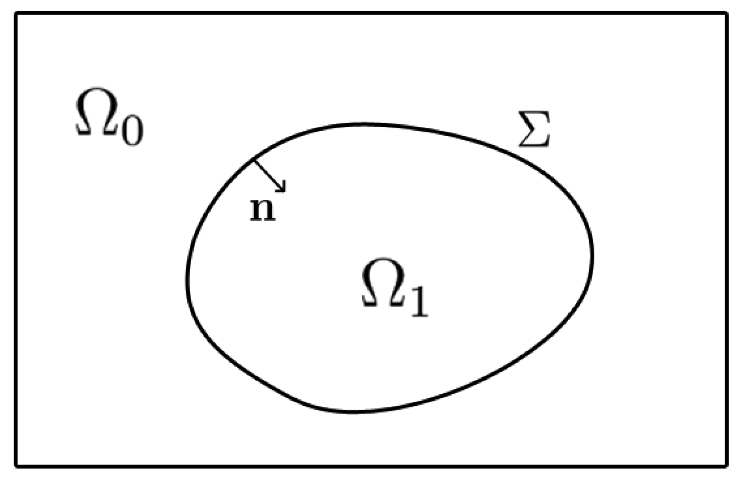
Let us consider the original domain of interest denoted by ${\Omega }_0$, typically the fluid domain, which is embedded inside a simple computational domain $\Omega \subset {\mathbb{R}}^d$. The auxiliary domain ${\Omega }_1$, typically a solid particle or an obstacle, is then such that $\Omega ={\Omega }_0\cup \Sigma \cup {\Omega }_1$ where $\Sigma$ is an immersed interface (see Figure 1). Let $\mathbf{n}$ be the unit outward normal vector to ${\Omega }_0$ on $\Sigma$. Our objective is to numerically impose the adequate boundary or interface conditions on the interface $\Sigma$. The continuous $L^2$-penalty method for the incompressible Navier–Stokes equations consists in adding a term $\frac{\chi }{\epsilon }(\mathbf{u}-{\mathbf{u}}_D)$ into the momentum equation

$$\rho (\frac{\partial \mathbf{u}}{\partial t}+(\mathbf{u}·\nabla )\mathbf{u})=-\nabla p+\rho \mathbf{g}+\nabla ·\left[\mu (\nabla \mathbf{u}+{\nabla }^T\mathbf{u})\right]+\frac{\chi }{\epsilon }(\mathbf{u}-{\mathbf{u}}_D)$$

(14)

where $0<\epsilon \ll 1$ denotes the penalty parameter and $\chi$ is the Heaviside function such as

$$\chi \left(x\right)=\{\begin{array}{c}1 \mathrm{if} x\in {\Omega }_1\\ 0 \mathrm{if} x\in {\Omega }_0.\end{array}$$

In ${\Omega }_0$, the penalty term vanishes and the original momentum equation is retrieved. In ${\Omega }_1$, the equation tends to $\mathbf{u}={\mathbf{u}}_D$ when $\epsilon ⟶0$. One can notice that the term used in [34] uses a coefficient similar to the penalty term but in the frame of a Chimera method where the coupling between two overlapping grids is performed.

3.2. Discretization

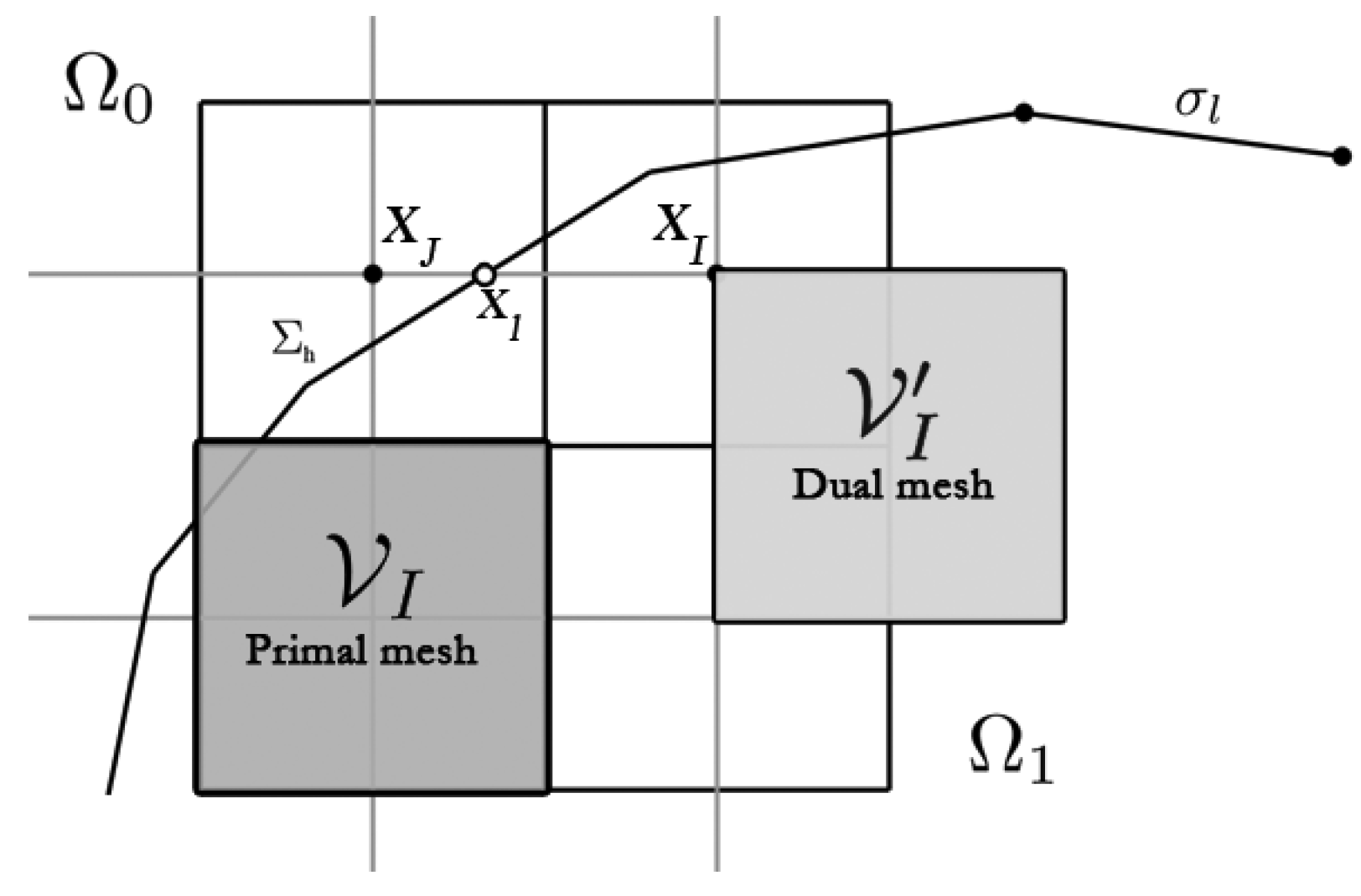
For the sake of simplicity, the method is described in 2D for a scalar equation. The computational domain $\Omega$ is approximated with a curvilinear mesh $T_h$ composed of $N\times M$ ($\times L$ in 3D) cell-centered finite volumes (${\mathcal{V}}_I$) for $I\in \mathcal{E}$, $\mathcal{E}$ being the set of index of the Eulerian orthogonal curvilinear structured mesh. Let $x_I$ be the vector coordinates of the center of each volume ${\mathcal{V}}_I$. The local characteristic space step $h_I$ of the volume ${\mathcal{V}}_I$ is defined as the maximum length of ${\mathcal{V}}_I$ in each direction, whereas h denotes the Eulerian mesh step: $h={sup}_{I\in \mathcal{E}}{h}_I$. This grid is used to discretize the conservation equations. A dual grid is introduced for the management of the penalty method (in finite-difference discretization, the primal mesh is used). The grid lines of this dual cell-vertex mesh are defined by the network of the cell centers $x_I$. The volumes of the dual mesh are denoted by ($K_I$). The Eulerian unknowns are noted ${\varphi }_I$ which are the approximated values of $\varphi \left(x_I\right)$, i.e. The solution at the cell centers $x_I$.

The discrete interface ${\Sigma }_h$, hereafter called the Lagrangian mesh, is given by a discretization of the original interface $\Sigma$. It is described by a piecewise linear approximation of $\Sigma$: ${\Sigma }_h=\{{\sigma }_l\in {\mathbb{P}}_1^{d-1},l\in {\mathcal{L}}_f\}$, K being the cardinal of ${\mathcal{L}}_f$ and ${\mathcal{L}}_f$ being the set of index of the Lagrangian mesh. Typically, ${\sigma }_l$ are segments in $2D$ and triangles in $3D$. The vertices of each face ${\sigma }_l$ are denoted by $x_{l,i}$ for $i=1,d$ and the set of all vertices is: $\{x_l,l\in {\mathcal{L}}_v\}$. The intersection points between the grid lines of the Eulerian dual mesh and the faces ${\sigma }_l$ of the Lagrangian mesh are denoted by $\{x_i,i\in \mathcal{I}\}$ (see Figure 2).

The cell centers $x_I$ are sorted according to their location inside ${\Omega }_0$ or ${\Omega }_1$ with the discrete Heaviside function ${\chi }_I=\chi \left(x_I\right)$. This function is computed from ${\Sigma }_h$ with a thread ray-casting method [35]. The principle is to cast a ray from each Eulerian nodes. If the number of intersections between ${\Sigma }_h$ and the ray is odd, the node is inside the object, otherwise outside. The algorithm needs $LMNK/max(L,M,N)$ intersection tests and is faster than the classical ray-casting method [36] which requires $LMNK$ intersection tests. New sets of Eulerian points $x_I$ are defined near the interface such as one neighbor $x_J$ verifying ${\chi }_J\ne {\chi }_I$ exists, i.e., the segment $[x_I;x_J]$ is cut by ${\Sigma }_h$. These Eulerian “interface” points are also sorted according to their location inside ${\Omega }_0$ or ${\Omega }_1$. Two sets $\{x_I,I\in {\mathcal{N}}_0\}$ and $\{x_I,I\in {\mathcal{N}}_1\}$ are so obtained, where ${\mathcal{N}}_0=\{I,x_I\in {\Omega }_0,\exists neighb\left(x_I\right)\in {\Omega }_1\}$ and ${\mathcal{N}}_1=\{I,x_I\in {\Omega }_1,\exists neighb\left(x_I\right)\in {\Omega }_0\}$.

The spatial order of the $L^2$-penalty method directly depends on the discretization of $\frac{\chi }{\epsilon }(\varphi -{\varphi }_D)$. The VPM [37] discretizes the term for a node ${\varphi }_i$ as $\frac{{\chi }_i}{\epsilon }({\varphi }_i-{\varphi }_D)$ with ${\varphi }_D$ the boundary value at the vicinity of $x_i$. As the solution is considered as constant in each penalized cells, the shape of the immersed boundary is perceived by the fluid as being stair-stepped, or rasterized. This inaccurate description of the interface implies a first-order of spatial convergence [38].

To reach a second-order of spatial accuracy, the sub-mesh penalty method (SMPM) [13,14] discretizes the penalty term with $\frac{{\chi }_i}{\epsilon }({\Pi }_i\varphi -{\varphi }_D\left(x_l\right))$ where ${\Pi }_i$ is a polynomial interpolator.

We consider a point $x_I$ with $I\in {\mathcal{N}}_1$ and only one neighbor $x_J$ in ${\Omega }_0$. The Lagrangian point $x_l$ is the intersection between $[x_I;x_J]$ and ${\Sigma }_h$ (Figure 2). The solution $\varphi ={\varphi }_l$ has to be satisfied at $x_l$ which implies in a discrete point of view ${\Pi }_I\varphi \left(x_l\right)={\varphi }_D\left(x_l\right)$ with $\Pi$ the ${\mathbb{P}}_1^1$-interpolator (one-dimensional linear polynomial) between the Eulerian unknowns $u_I$ and $u_J$:

$${\varphi }_l={\alpha }_I{\varphi }_I+{\alpha }_J{\varphi }_J \mathrm{with} 0<{\alpha }_I,{\alpha }_J<1 \mathrm{and} {\alpha }_I+{\alpha }_J=1$$

(15)

The coefficients ${\alpha }_I$ and ${\alpha }_J$ are determined such as ${\Pi }_I\varphi \left(x_I\right)={\varphi }_I$ and ${\Pi }_I\varphi \left(x_J\right)={\varphi }_J$. If now $x_I$ has a second neighbor $x_K$ in ${\Omega }_0$, the intersection $x_m$ between $[x_I;x_K]$ and ${\Sigma }_h$ is considered. We choose $x_p$, a new point of ${\Sigma }_h$ between $x_l$ and $x_m$ (see Figure 1). Practically, the barycenter between $x_m$ and $x_l$ is used. The resulting point $x_p$ is not necessarily on ${\Sigma }_h$ but it does not spoil the second-order precision of the method since the distance $d(x_p,{\Sigma }_h)$ between $x_p$ and ${\Sigma }_h$ is varying as $\mathcal{O}\left(h^2\right)$. The solution ${\varphi }_p\left(x_p\right)$ is then approximated using a ${\mathbb{P}}_1^2$-interpolation (two-dimensional linear polynomial) of the values ${\varphi }_I$, ${\varphi }_J$ and ${\varphi }_K$:

$${\varphi }_p={\alpha }_I{\varphi }_I+{\alpha }_J{\varphi }_J+{\alpha }_K{\varphi }_K,0<{\alpha }_I,{\alpha }_J,{\alpha }_K<1,{\alpha }_I+{\alpha }_J+{\alpha }_K=1$$

(16)

We can also use a ${\mathbb{Q}}_1^2$-interpolation of ${\varphi }_I$, ${\varphi }_J$, ${\varphi }_K$ and ${\varphi }_L$, by extending the interpolation stencil with the point $x_L$ which is the fourth point of the cell of the dual mesh defined by $x_I$, $x_J$, and $x_K$ (see Figure 2).

If ${\Sigma }_h$ is regular enough, $x_I$ has almost never a third neighbor in ${\Omega }_0$. However, if it is the case, the first-order $L^2$-penalty term $\frac{{\chi }_I}{\epsilon }({\varphi }_I-{\varphi }_D\left(x_l\right))$ is used. In any case, by decreasing the Eulerian mesh step h, we also decrease the number of points $x_I$ having more than two neighbors in ${\Omega }_0$.

It has to be noticed that the penalty term is only required for nodes $x_I$ with $I\in {\mathcal{N}}_1$, i.e., for the nodes in ${\Omega }_1$ with at least one neighbor in ${\Omega }_0$. What happens inside ${\Omega }_1$ and far from $\Sigma$ has no impact on the flow in ${\Omega }_0$ and so is of secondary interest (practically, the parts of the discretization matrix corresponding to these nodes are removed before the resolution of the linear system).

Concerning the application of the method to a Curvilinear grid, the computational domain can be “unfold” into a Cartesian domain where most of the computations are performed. Hence, the penalty constraints are build from the Cartesian grid with the standard Cartesian routines. The curvilinear to Cartesian projection is described in [35].

4. Penalty Correction for the Pressure Correction Methods

4.1. First-Order Correction

For a first-order penalty term, such a correction is easy to perform [23]. Let us now write the momentum Navier–Stokes equation with a first-order penalty term:

$$\rho \frac{\partial \mathbf{u}}{\partial t}=+RHS-\nabla p+\frac{\chi }{\epsilon }(\mathbf{u}-{\mathbf{u}}_D)$$

(17)

In the standard method, Equations (4) and (5) are considered to obtain Equation (6). The same operation is performed with the penalty term and Equation (6) becomes

$$\rho \left(\frac{{\mathbf{u}}^{n+1}-{\mathbf{u}}^{*}}{\Delta t}\right)=-\nabla p^{\prime }+\frac{\chi }{\epsilon }({\mathbf{u}}^{n+1}-{\mathbf{u}}^{*})$$

(18)

while Equation (7) becomes

$$\nabla ·{\mathbf{u}}^{*}=\nabla ·{(\frac{\Delta t}{\rho }-\frac{\chi }{\epsilon })}^{-1}\nabla p^{\prime }.$$

(19)

The velocity is then updated using Equation (18):

$${\mathbf{u}}^{n+1}={\mathbf{u}}^{*}-{(\frac{\Delta t}{\rho }-\frac{\chi }{\epsilon })}^{-1}\nabla p^{\prime }.$$

(20)

It is important to notice that the correction terms due to the fictitious domain method appears naturally with this walkthrough. The standard pressure update is not modified.

Remark 1.

A classical problem with the elliptic Equation (19) in the penalized approach is that the diffusion coefficient varies in $O\left({\epsilon }^{-1}\right)$ in ${\Omega }_1$. Hence, a strong imposition of the penalty constraint produces a very high diffusion coefficient which leads to instabilities due to issues of numerical accuracy. In [24], with the assumption that ρ is constant over the domain, the authors proposed the following correction to avoid numerical instabilities:

$$\frac{\rho }{\Delta t}\nabla ·{\mathbf{u}}^{*}=\nabla ·\frac{\epsilon }{\epsilon +\chi }\nabla p^{n+1}+\frac{1}{\epsilon }(p^{n+1}-p^0)$$

(21)

where $p^0$ is a prescribed pressure. The last term produces a $L^2$-penalization of the pressure equation.

Remark 2.

In [24], the authors used the non-incremental version of the scheme and a first-order correction for the pressure equation. However, the boundary condition is explicitly chosen as being the linear extrapolation of the solution and a second-order of spatial convergence is reached for a stationary case. In our approach, all the terms due to the penalization are of second-order and implicit.

4.2. Higher-Order Correction

A fully implicit second-order correction is now proposed. A consistent correction following the precedent walkthrough with a penalty term of higher order is much more delicate. The first-order term $\frac{{\chi }_i}{\epsilon }({\mathbf{u}}_i-{\mathbf{u}}_D\left(x_l\right))$ is replaced by $\frac{{\chi }_i}{\epsilon }({\Pi }_i\mathbf{u}-{\mathbf{u}}_D\left(x_l\right))$ with ${\Pi }_i\mathbf{u}={\displaystyle \sum _{j/x_j\in Neighb\left(x_i\right)}}{\alpha }_j{\mathbf{u}}_j$. The pressure in Equation (19) becomes, for each node $x_i$:

$$\nabla ·{\mathbf{u}}_i^{*}=\nabla ·{(\frac{\rho }{\Delta t}-\frac{{\chi }_i}{\epsilon }{\Pi }_i)}^{-1}\nabla p^{\prime }$$

(22)

which requires the calculation of the matrix corresponding to ${(\frac{\rho }{\Delta t}-\frac{{\chi }_i}{\epsilon }{\Pi }_i)}^{-1}$ before the resolution of the initial system. A more simple method is presented here even if it would be interesting to evaluate this first method. We start back with Equation (6) with a penalty term by following the natural walkthrough of the first-order correction:

$${\mathbf{u}}_i^{n+1}-{\mathbf{u}}_i^{*}=-\frac{\Delta t}{\rho }\nabla p^{\prime }+\frac{\Delta t{\chi }_i}{\rho \epsilon }{\Pi }_i({\mathbf{u}}^{n+1}-{\mathbf{u}}^{*})$$

(23)

developed as

$$(1-\frac{\Delta t{\chi }_i}{\rho \epsilon }{\Pi }_i)({\mathbf{u}}^{*}-{\mathbf{u}}^{n+1})=\frac{\Delta t}{\rho }\nabla p^{\prime }.$$

(24)

The key of this construction is to introduce ${\Pi }_i^{\prime }$, a new interpolator such as:

$${\Pi }_i^{\prime }\mathbf{u}=\sum _{j/x_j\in Neighb\left(x_i\right),i\ne j}{\alpha }_j{\mathbf{u}}_j.$$

(25)

Hence, ${\Pi }_i\mathbf{u}={\alpha }_i{\mathbf{u}}_i+{\Pi }_i^{\prime }\mathbf{u}$ and we have

$$(1-\frac{\Delta t{\chi }_i}{\rho \epsilon }({\alpha }_i+{\Pi }_i^{\prime }))({\mathbf{u}}^{*}-{\mathbf{u}}^{n+1})=\frac{\Delta t}{\rho }\nabla p^{\prime }.$$

(26)

By construction, the nodes involved by ${\Pi }_i^{\prime }$ are always in ${\Omega }_0$ where $\chi =0$ so the original pressure-correction method occurs. Hence, using Equation (9), we have

$$(1-\frac{\Delta t{\chi }_i{\alpha }_i}{\rho \epsilon })({\mathbf{u}}_i^{*}-{\mathbf{u}}_i^{n+1})-(\frac{\Delta t{\chi }_i}{\rho \epsilon }{\Pi }_i^{\prime }\frac{\Delta t}{\rho }\nabla p^{\prime })=\frac{\Delta t}{\rho }\nabla p^{\prime }$$

(27)

and we obtain

$${\mathbf{u}}_i^{n+1}={\mathbf{u}}_i^{*}-(\frac{\Delta t{\chi }_i}{\rho \epsilon -\Delta t{\chi }_i{\alpha }_i}{\Pi }_i^{\prime }\frac{\Delta t}{\rho }\nabla p^{\prime }+\frac{\Delta t{\epsilon }_i}{\rho \epsilon -\Delta t{\chi }_i{\alpha }_i}\nabla p^{\prime }).$$

(28)

the equation of the velocity update. Using the divergence of Equation (28) and $\nabla ·{\mathbf{u}}_i^{n+1}=0$ we obtain the final correction equation

$$\nabla ·{\mathbf{u}}_i^{*}=\nabla ·(\frac{\Delta t{\chi }_i}{\rho \epsilon -\Delta t{\chi }_i{\alpha }_i}{\Pi }_i^{\prime }\frac{\Delta t}{\rho }\nabla p^{\prime }+\frac{\Delta t{\epsilon }_i}{\rho \epsilon -\Delta t{\chi }_i{\alpha }_i}\nabla p^{\prime }).$$

(29)

The parameter $\epsilon \ll 1$ and we obtain at the limit:

$$\frac{\Delta t{\chi }_i}{\rho \epsilon -\Delta t{\chi }_i{\alpha }_i}⟶0 \mathrm{and} \frac{\Delta t\epsilon }{\rho \epsilon -\Delta t{\chi }_i{\alpha }_i}⟶\frac{\Delta t}{\rho } \mathrm{in} {\Omega }_0 \mathrm{when} \epsilon ⟶0$$

(30)

as $\chi \left(x_i\right)=0$ for $x_i\in {\Omega }_0$ and

$$\frac{\Delta t{\chi }_i}{\rho \epsilon -\Delta t{\chi }_i{\alpha }_i}⟶-\frac{1}{{\alpha }_i} \mathrm{and} \frac{\Delta t\epsilon }{\rho \epsilon -\Delta t{\chi }_i{\alpha }_i}⟶0 \mathrm{in} {\Omega }_1 \mathrm{when} \epsilon ⟶0.$$

(31)

The pressure update is still $p^{n+1}=p^n+p^{\prime }(-\mu \nabla ·{\mathbf{u}}^{*})$. Using Equation (23) to build the velocity update, the standard in Equation (9) is recovered in ${\Omega }_0$.

A major advantage of this formulation is that the diffusion coefficient in the pressure in Equation (29) has generally an absolute value of magnitude $\Delta t/\rho$ which avoid the numerical instability of the first-order method. Critical values appears when the interface is very close to the penalized node or a neighbor of the penalized node. If we consider the case where a node $x_I\in {\Omega }_1$ has one neighbor $x_J\in {\Omega }_0$, the penalty constraint is ${\alpha }_I{\mathbf{u}}_I+(1-{\alpha }_I){\mathbf{u}}_J={\mathbf{u}}_D\left(x_l\right)$, and here ${\Pi }_I^{\prime }\mathbf{u}=(1-{\alpha }_I){\mathbf{u}}_J$. Hence, the diffusion coefficient is $({\alpha }_I-1)\Delta t/\left({\alpha }_I\rho \right)$ and is critical if the interface ${\Sigma }_h$ is close to the penalized node. In this case, the coefficient is very small and the same problem as with the first-order correction occurs. However, we noticed that a correct solution can be obtained with a diffusion coefficient of magnitude ${10}^{-10}$. If the interface position leads to a smaller value, one can slightly move the interface to decrease ${\alpha }_I$. The case ${\alpha }_I\ll 1$ provides a large diffusion coefficient and produces a $H^1$-penalty term [11], that is to say a Neumann boundary condition in the considered cell.

4.3. Comparison to the Ikeno–Kajishima Correction

This approach was proposed by Hikeno and Kajishima [20] for a DF-IBM method and is presented here for our interpolator $\Pi$. They propose the following velocity update

$${\mathbf{u}}_i^{n+1}={\mathbf{u}}_i^{*}-((1-{\chi }_i)\frac{\Delta t}{\rho }\nabla p^{\prime }-{\chi }_i{\displaystyle \frac{{\Pi }_i^{\prime }\frac{\Delta t}{\rho }\nabla p^{\prime }}{{\alpha }_i}})$$

(32)

which is directly introduced and not obtained from the solved momentum equation (the consistency of the method is demonstrated afterwards). In our formulation, all the method is derived from the original momentum equation and the prediction equation so the consistency is naturally deduced. From Equation (32) and the incompressibility constraint, the following equation is obtained:

$$\nabla ·{\mathbf{u}}_i^{*}=\nabla ·((1-{\chi }_i)\frac{\Delta t}{\rho }\nabla p^{\prime }-{\chi }_i{\displaystyle \frac{{\Pi }_i^{\prime }\frac{\Delta t}{\rho }\nabla p^{\prime }}{{\alpha }_i}}).$$

(33)

and the pressure is updated as in the standard method

$$p^{n+1}=p^{\prime }+p^n.$$

(34)

The method is applied too to the non-incremental fractional step method.

As can be seen, the equations obtained are different than with the present approach. Obviously, it is due to the way the boundary condition is imposed (penalty term with a coefficient $1/\epsilon$ of dominant magnitude in our case or IBM direct-forcing term with Dirac function in [20]). However, the final pressure correction equation with the penalized correction in Equation (29) tends to Equation (33) when $\epsilon$ tends to zero. The same result is obtained with the corresponding velocity updates.

Remark 3.

For this correction (and the penalty correction presented here when $\epsilon \to 0$), the velocity in ${\Omega }_1$ is updated as

$${\mathbf{u}}_i^{n+1}={\mathbf{u}}_i^{*}+{\displaystyle \frac{{\Pi }_i^{\prime }\frac{\Delta t}{\rho }\nabla p^{\prime }}{{\alpha }_i}}$$

(35)

By construction of the interpolator ${\Pi }_i\mathbf{u}={\alpha }_i{\mathbf{u}}_i+{\Pi }_i^{\prime }\mathbf{u}$, no node of ${\Omega }_1$ is involved in ${\Pi }_i^{\prime }$. Hence, as the pressure correction in ${\Omega }_0$ is

$${\mathbf{u}}_i^{n+1}={\mathbf{u}}_i^{*}-\frac{\Delta t}{\rho }\nabla p^{\prime },$$

(36)

one can replace ${\displaystyle \frac{\Delta t}{\rho }}\nabla p^{\prime }$ by $({\mathbf{u}}_i^{*}-{\mathbf{u}}_i^{n+1})$ to obtain

$${\mathbf{u}}_i^{n+1}={\mathbf{u}}_i^{*}-{\displaystyle \frac{{\Pi }_i^{\prime }({\mathbf{u}}_i^{*}-{\mathbf{u}}_i^{n+1})}{{\alpha }_i}}.$$

(37)

Considering the initial interpolator ${\Pi }_i$, we obtain

$${\Pi }_i{\mathbf{u}}_i^{n+1}={\Pi }_i{\mathbf{u}}_i^{*}$$

(38)

and the boundary constraint obtained in the predictor step is conserved. It induces as well that ${\Pi }_i{\mathbf{u}}_i^{\prime }=0$. The update of the velocity near the velocity is not necessarily null contrary to the linear combination of these velocities.

4.4. Temporal Accuracy for the Incremental Pressure-Correction

We study here the temporal accuracy of the pressure for the penalized incremental pressure-correction method with a first-order Euler scheme. The temporal accuracy for the base method is $O(\Delta t)$ [30]. The ideal equation system to solve is:

$$\left[\begin{array}{cc}A& G\\ D& 0\end{array}\right]\left[\begin{array}{c}{\mathbf{u}}^{n+1}\\ p^{n+1}\end{array}\right]=\left[\begin{array}{c}r\\ 0\end{array}\right]$$

(39)

with G the gradient operator, D the divergence operator, and A the following sub-matrix

$$A=\left\{\frac{\rho }{\Delta t}+N-V-\frac{\chi }{\epsilon }\Pi \right\}$$

(40)

with N the linearized discretization of the inertial term and V the discretization of the viscous term. The second member r is defined as

$$r_i=\frac{\Delta t}{\rho }{\mathbf{u}}_i^{*}-\frac{{\chi }_i}{\epsilon }{\Pi }_i{\mathbf{u}}^{*}.$$

(41)

The velocity update in Equation (28) allows writing

$$\left[\begin{array}{cc}I& BG\\ 0& I\end{array}\right]\left[\begin{array}{c}{\mathbf{u}}^{n+1}\\ p^{n+1}\end{array}\right]=\left[\begin{array}{c}{\mathbf{u}}^{*}\\ p^{n+1}\end{array}\right]$$

(42)

with I the identity matrix and B the matrix such as

$$B=\left\{\frac{\Delta t{\chi }_i}{\rho \epsilon -\Delta t{\chi }_i{\alpha }_i}{\Pi }_i^{\prime }\frac{\Delta t}{\rho }+\frac{\Delta t\epsilon }{\rho \epsilon -\Delta t{\chi }_i{\alpha }_i}\right\}.$$

(43)

At last, the pressure elliptic equation yields

$$\left[\begin{array}{cc}A& 0\\ D& -DBG\end{array}\right]\left[\begin{array}{c}{\mathbf{u}}^{*}\\ p^{n+1}\end{array}\right]=\left[\begin{array}{c}r\\ 0\end{array}\right].$$

(44)

As first noticed by Perot [39], the two systems in Equations (42) and (44) are a block $LU$ decomposition of the system

$$\left[\begin{array}{cc}A& ABG\\ D& 0\end{array}\right]\left[\begin{array}{c}{\mathbf{u}}^{n+1}\\ p^{n+1}\end{array}\right]=\left[\begin{array}{c}r\\ 0\end{array}\right]$$

(45)

which allows us to write the error of the scheme using Equation (39):

$$AB=\left\{(\frac{\rho }{\Delta t}+N-V-\frac{\chi }{\epsilon }\Pi )(\frac{\Delta t\chi }{\rho \epsilon -\Delta t\chi \alpha }{\Pi }^{\prime }\frac{\Delta t}{\rho }+\frac{\Delta t\epsilon }{\rho \epsilon -\Delta t\chi \alpha })\right\}.$$

(46)

We study the error in ${\Omega }_0$. We consider the matrices $N_0$, $N_1$, $V_0$ and $V_1$ such as $V=V_0+V_1$ and $N=N_0+N_1$. The matrix $N_0$ is such that ${\left\{N_0\right\}}_{i,j}={\left\{N\right\}}_{i,j}$ if $x_j\in {\Omega }_0$, else ${\left\{N_0\right\}}_{i,j}=0$. The same occurs for $V_0$. It is necessary to split these contributions as the value of $\chi$ varies in B. Hence, we have

$$AB=\left\{(\frac{\rho }{\Delta t}+N_0-V_0)\frac{\Delta t}{\rho }+(N_1-V_1)(\frac{\Delta t}{\rho \epsilon -\Delta t\alpha }{\Pi }^{\prime }\frac{\Delta t}{\rho }+\frac{\Delta t\epsilon }{\rho \epsilon -\Delta t\alpha })\right\}$$

(47)

which tends to term in $\{1+O(\Delta t\left)\right\}$ when $\epsilon$ tends to zero. The first order is retrieved. We consider now the error in ${\Omega }_1$:

$$\begin{array}{lll}AB& =& \left\{(N_0-V_0-\frac{1}{\epsilon }{\Pi }^{\prime })\frac{\Delta t}{\rho }+(\frac{\rho }{\Delta t}+N_1-V_1-\frac{1}{\epsilon }\alpha )(\frac{\Delta t}{\rho \epsilon -\Delta t\alpha }{\Pi }^{\prime }\frac{\Delta t}{\rho }+\frac{\Delta t\epsilon }{\rho \epsilon -\Delta t\alpha })\right\}\\ & =& \{(N_0-V_0)\frac{\Delta t}{\rho }+(-\frac{1}{\epsilon }+\frac{\rho }{\rho \epsilon -\Delta t\alpha }-\frac{\Delta t\alpha }{\epsilon (\rho \epsilon -\Delta t\alpha )}){\Pi }^{\prime }\frac{\Delta t}{\rho }\\ & & +(N_1-V_1)(\frac{\Delta t}{\rho \epsilon -\Delta t\alpha }{\Pi }^{\prime }\frac{\Delta t}{\rho }+\frac{\Delta t\epsilon }{\rho \epsilon -\Delta t\alpha })+\frac{\rho \epsilon }{\rho \epsilon -\Delta t\alpha }-\frac{\Delta t\alpha }{\rho \epsilon -\Delta t\alpha }\}\\ & =& \{(N_0-V_0)\frac{\Delta t}{\rho }+(N_1-V_1)(\frac{\Delta t}{\rho \epsilon -\Delta t\alpha }{\Pi }^{\prime }\frac{\Delta t}{\rho }+\frac{\Delta t\epsilon }{\rho \epsilon -\Delta t\alpha })+1\}\end{array}$$

(48)

which also tends to a term in $\{1+O(\Delta t\left)\right\}$ when $\epsilon$ tends to zero. Hence, the order of the original method is retrieved. The same result with a quite similar analysis is obtained by [20].

4.5. Value of the Penalty Parameter

The value of the penalty parameter $\epsilon$ has an influence on the solution as the solution ${\mathbf{u}}^{*}$ obtained with the momentum equations converges toward the desired solution for the $L^2$-norm with an order ≤3/4 in $\epsilon$ [11].

For the first-order method, the value of the parameter is more critical. In the present approach, the empirical value $\epsilon \approx {10}^{-10}$ is used. This value can vary depending on the linear solver. Nonetheless, taking $\epsilon \approx {10}^{-20}$ in Equation (20) ensures the desired velocity inside the obstacle. For the second-order correction, $\epsilon$ can be taken sufficiently small to ensure $\Pi {\mathbf{u}}^{*}={\mathbf{u}}_D$ at machine accuracy when the high-order penalty term is used. The converged correction can be also directly implemented.

5. Numerical Experiments

The performances of the modified pressure-correction are evaluated here. The method is compared to the augmented Lagrangian method which does not require a correction. It is also an opportunity to compare the approaches in a more general point of view. When no analytical solution is available, a Richardson extrapolation is used to compute a reference solution [40]. We consider three values $h_1$, $h_2$, and $h_3$ of a numerical parameter verifying consecutive ratios of two. The convergence rate $\theta$ and the reference solution $f_{ext}$ are given by:

$$\theta =\frac{ln\left(\frac{f_{h_1}-f_{h_2}}{f_{h_2}-f_{h_3}}\right)}{ln\left(\frac{h_1}{h_2}\right)}$$

(49)

$$f_{ext}=\frac{{\left(\frac{h_2}{h_3}\right)}^{\theta }{f}_{h_3}-f_{h_2}}{{\left(\frac{h_2}{h_3}\right)}^{\theta }-1}$$

(50)

The asymptotical convergence zone has to be reached to obtain a relevant extrapolation.

5.1. Cylindrical Couette Flow

We consider a Couette flow between two cylinders of radius $R_1=0.5$ m and $R_2=3$ m. Their angular velocities are ${\omega }_1=0$ rad·s${}^{-1}$ and ${\omega }_2=2$ rad·s${}^{-1}$. The solution is

$$v_{\theta }\left(r\right)=\frac{{\omega }_2{R}_2^2-{\omega }_1{R}_1^2}{R_2^2-R_1^2}r+\frac{({\omega }_1-{\omega }_2)R_2^2{R}_1^2}{R_2^2-R_1^2}\frac{1}{r}$$

(51)

for the velocity and

$$p\left(r\right)=\rho a^2\frac{r^2}{2}-\frac{b^2}{2r^2}+2ablog\left(r\right)$$

(52)

for the pressure with

$$a=\frac{{\omega }_2{R}_2^2-{\omega }_1{R}_1^2}{R_2^2-R_1^2} \mathrm{and} b=({\omega }_1-{\omega }_2)\frac{R_1^2{R}_2^2}{R_2^2-R_1^2}.$$

The NS equations are solved in a domain $\Omega =[-2;2+0.1\sqrt{2}]\times [-2;2+0.2\sqrt{2}]$. The analytical solution is imposed on $\partial \Omega$. The SMP method is used to impose a Dirichlet BC on the inner circle. For the augmented Lagrangian method, a value of the parameter $dr=10$ is chosen.

The convergence study of the $L^2$ relative spatial error for the second-order correction is given in

Table 1. $L^2$ relative errors in space and corresponding orders for the velocity and the pressure— rotational pressure-correction method with second-order correction.

Mesh	${\mathit{L}}^2$ Rel. Error. u	Order	${\mathit{L}}^2$ Rel. Error. p	Order	Iter NS	Iter SPT
16	$3.409\times {10}^{-3}$		$5.898\times {10}^{-3}$		8.77	31.9
32	$4.708\times {10}^{-4}$	$2.86$	$4.222\times {10}^{-3}$	$0.48$	19.2	67.0
64	$1.307\times {10}^{-4}$	$1.85$	$1.269\times {10}^{-3}$	$1.73$	38.7	115
128	$\times {10}^{-5}$	$1.98$	$3.979\times {10}^{-4}$	$1.67$	91.6	384
256	$8.032\times {10}^{-6}$	$2.04$	$1.339\times {10}^{-4}$	$1.57$	195	2036
512	$2.111\times {10}^{-6}$	$1.93$	$5.040\times {10}^{-5}$	$1.41$	430
1024	$5.281\times {10}^{-7}$	$2.00$	$2.040\times {10}^{-5}$	$1.30$	1072	1059

and plotted in Figure 3. These results are obtained with the rotational pressure-correction (same results with a negligible differential on the $L^2$ error are obtained with the AL method) demonstrating the spatial accuracy of the modification. As expected for such a case [14], a second order is obtained for the velocity. The convergence rate for the pressure error is around $1.5$. These results are compared with the first-order correction (

Table 2. $L^2$ relative errors in space and corresponding orders for the velocity and the pressure— rotational pressure-correction method with first-order approach.

Mesh	${\mathit{L}}^2$ Rel. Error. u	Order	${\mathit{L}}^2$ Rel. Error. p	Order	Iter NS	Iter SPT
16	$2.374\times {10}^{-2}$		$7.796\times {10}^{-2}$		8.35	14.7
32	$1.317\times {10}^{-2}$	$0.85$	$5.620\times {10}^{-2}$	$0.47$	19.0	28.4
64	$5.239\times {10}^{-3}$	$1.33$	$3.471\times {10}^{-2}$	$0.69$	64.6	59.8
128	$2.357\times {10}^{-3}$	$1.15$	$2.479\times {10}^{-2}$	$0.49$	77	114
256	$1.043\times {10}^{-3}$	$1.18$	$1.955\times {10}^{-2}$	$0.34$	156	223
512	$4.420\times {10}^{-4}$	$1.24$	$1.342\times {10}^{-2}$	$0.54$	323	472
1024	$2.057\times {10}^{-4}$	$1.10$	$9.597\times {10}^{-3}$	$0.48$	696	1100

) where an order slightly superior to one is obtained for the velocity and a $0.5$ order is obtained for the pressure. For both tables, the average number of solver iterations for the 30 first iterations is shown. The additional cost for the high-order method varies according to the mesh as critical cases occur (when a diagonal term is very small compared to extra-diagonal terms, i.e., when ${\alpha }_I\ll {\alpha }_J$ in [15]) depends on the position of ${\Sigma }_h$ with respect to $T_h$. For the present case, the higher overcost for the pressure equation obtained with the ${256}^2$ mesh is greatly compensated by the higher accuracy of the solution. On can notice that critical cases can be removed at the expend of a slight loss of accuracy by slightly moving the interface.

Table 3. $L^2$ relative errors in space and corresponding orders for the velocity and the pressure—rotational pressure-correction method without correction for the pressure.

Mesh	${\mathit{L}}^2$ Rel. Error. u	Order	${\mathit{L}}^2$ Rel. Error. p	Order
16	$5.652\times {10}^{-3}$		$9.144\times {10}^{-3}$
32	$1.451\times {10}^{-3}$	$1.96$	$4.376\times {10}^{-3}$	$1.06$
64	$5.242\times {10}^{-4}$	$1.47$	$1.322\times {10}^{-3}$	$1.73$
128	$1.412\times {10}^{-4}$	$1.89$	$4.052\times {10}^{-4}$	$1.71$
256	$5.260\times {10}^{-5}$	$1.42$	$1.357\times {10}^{-4}$	$1.58$
512	$1.673\times {10}^{-5}$	$1.65$	$5.036\times {10}^{-5}$	$1.43$
1024	$5.687\times {10}^{-6}$	$1.56$	$2.039\times {10}^{-5}$	$1.30$

gives the same convergence study for the rotational method without immersed-boundary correction for the pressure for a time step $\Delta t=1$ s. As can be seen in Figure 3, the lack of correction has almost no influence on the pressure. The convergence rate for the velocity is lower but acceptable. A factor ten is obtained between the solution with and without the correction for the finest mesh.

The time evolution of the solution is now evaluated. For a case with Dirichlet boundary conditions, the authors of [30,41] gave for the rotational method a rate of $O(\Delta t^2)$ for the velocity and $O(\Delta t^{\frac{3}{2}})$ for the pressure.

Simulations with a $64\times 64$ mesh are conducted with different time steps and velocity–pressure coupling methods. The instant $T_p$ when the $L^2$ error on the pressure reaches $1.5\times {10}^{-3}$ and the instant $T_v$ when the $L^2$ error on the velocity reaches $1.5\times {10}^{-4}$ are considered to study the convergence.

Table 4. Temporal convergence of the error on the velocity and the pressure for the augmented Lagrangian and the rotational pressure-correction methods—Gear 1 scheme for the Couette flow.

$\Delta \mathit{t}$	${\mathit{T}}_{\mathit{u}}$ AL	Order	${\mathit{T}}_{\mathit{p}}$ AL	Order	${\mathit{T}}_{\mathit{u}}$ SPT	Order	${\mathit{T}}_{\mathit{p}}$ SPT	Order
Ref.	2.107		1.863		2.107		1.863
$128\times {10}^{-3}$	$5.168\times {10}^{-1}$		$5.172\times {10}^{-1}$		$6.402\times {10}^{-1}$		$1.034\times {10}^0$
$64\times {10}^{-3}$	$2.591\times {10}^{-1}$	1.00	$2.584\times {10}^{-1}$	1.00	$2.835\times {10}^{-1}$	1.18	$2.968\times {10}^{-1}$	1.80
$32\times {10}^{-3}$	$1.315\times {10}^{-1}$	0.98	$1.304\times {10}^{-1}$	0.99	$1.353\times {10}^{-1}$	1.07	$1.381\times {10}^{-1}$	1.10
$16\times {10}^{-3}$	$6.630\times {10}^{-2}$	0.99	$6.539\times {10}^{-2}$	1.00	$6.651\times {10}^{-2}$	1.02	$6.654\times {10}^{-2}$	1.05
$8\times {10}^{-3}$	$3.328\times {10}^{-2}$	0.99	$3.268\times {10}^{-2}$	1.00	$3.299\times {10}^{-2}$	1.01	$3.259\times {10}^{-2}$	1.03
$4\times {10}^{-3}$	$1.665\times {10}^{-2}$	1.00	$1.636\times {10}^{-2}$	1.00	$1.640\times {10}^{-2}$	1.01	$1.614\times {10}^{-2}$	1.01
$2\times {10}^{-3}$	$8.339\times {10}^{-3}$	1.00	$8.185\times {10}^{-3}$	1.00	$8.182\times {10}^{-3}$	1.00	$8.019\times {10}^{-3}$	1.01
$1\times {10}^{-3}$	$4.177\times {10}^{-3}$	1.00	$4.096\times {10}^{-3}$	1.00	$4.082\times {10}^{-3}$	1.00	$3.984\times {10}^{-3}$	1.01

shows the convergence of these values for the augmented Lagrangian and rotational pressure-correction methods, and for the Euler temporal schemes. The reference values are computed with the Richardson extrapolation using the three more refined values. A clear first-order convergence is obtained for the velocity and the pressure for both velocity–pressure coupling methods. Except for the larger time-steps, both methods give the same results.

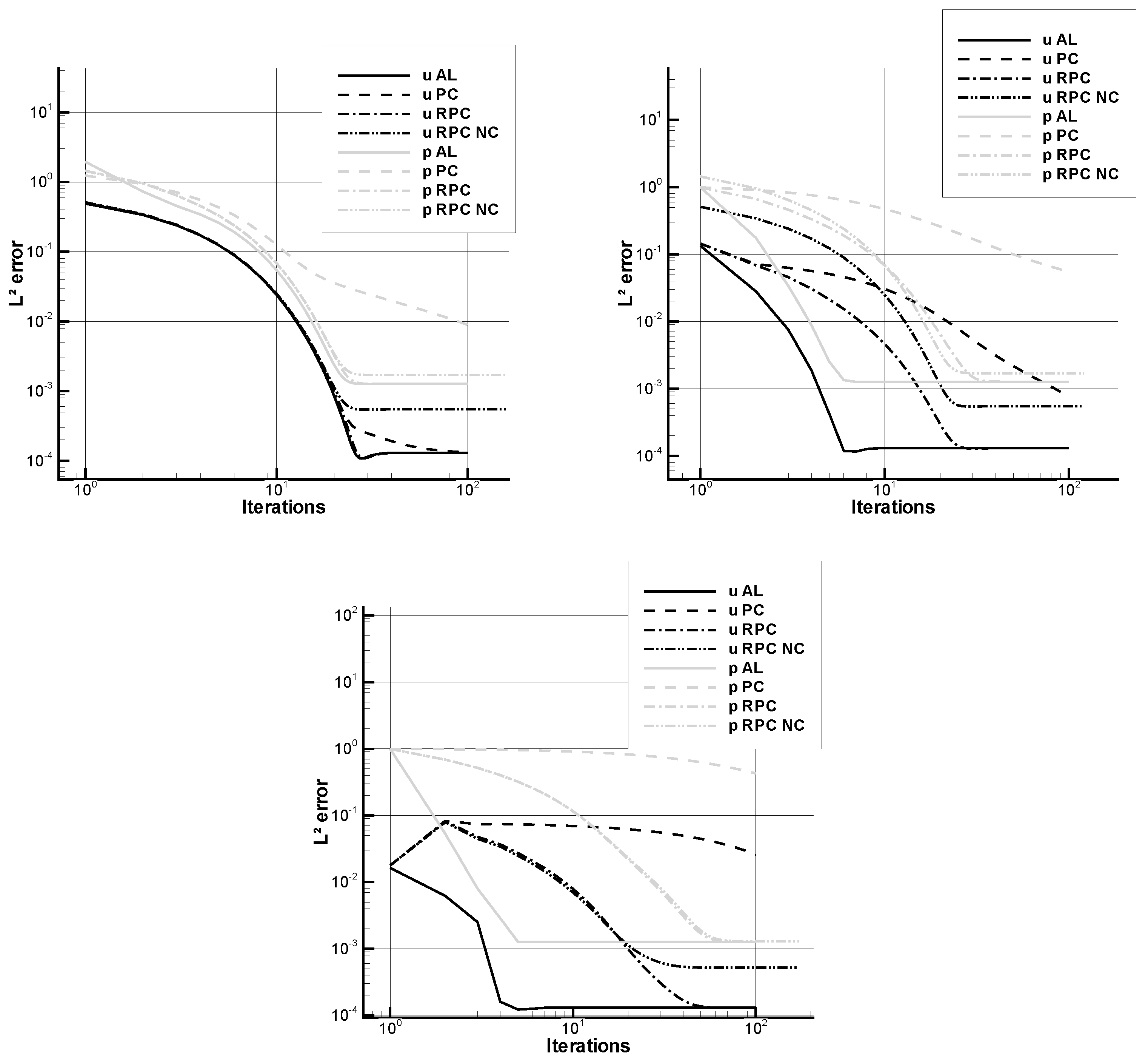
Figure 4 shows the evolution of the spatial error with respect to the number of time iterations for $\Delta t=0.1$ s, $\Delta t=1$ s, and $\Delta t=10$ s while

Table 5. Temporal convergence of the error on the velocity and the pressure for the augmented Lagrangian and the rotational pressure-correction methods for large time steps for the Couette flow.

$\Delta \mathit{t}$	${\mathit{T}}_{\mathit{v}}$ AL	${\mathit{T}}_{\mathit{p}}$ AL	${\mathit{T}}_{\mathit{v}}$ SPT	${\mathit{T}}_{\mathit{p}}$ SPT
10	42.27	47.76	439.8	538.2
1	5.801	5.811	24.18	29.99
$0.1$	2.506	2.266	2.573	2.4214

gives the values of $T_v$ and $T_p$ for these time steps. Due to its strong implicitation, the AL method is always converging faster than the pressure-corrections. One can notice that the temporal evolution of the solution for the rotational method without correction is quite similar to the evolution of the corrected methods up to an error of ${10}^{-3}$ on the velocity. For this case, the interest of the correction seems to be minor. Figure 4 shows that the convergence of the incremental pressure-correction is much slower than with the other methods. For the present case, reaching the same level of error as with the two others methods is prohibitive.

The curves of convergence for the second-order Gear scheme are shown in Figure 5 (the error convergence for the velocity with the augmented Lagrangian method and for the first-order temporal scheme is given for comparison). The values are given in

Table 6. Temporal convergence of the error on the velocity and the pressure for the augmented Lagrangian and the rotational pressure-correction methods—Gear 2 scheme for the Couette flow.

$\Delta \mathit{t}$	${\mathit{T}}_{\mathit{u}}$ AL	Order	${\mathit{T}}_{\mathit{p}}$ AL	Order	${\mathit{T}}_{\mathit{u}}$ SPT	Order	${\mathit{T}}_{\mathit{p}}$ SPT	Order
Ref.	2.107		1.863		2.107		1.863
$128\times {10}^{-3}$	$1.918\times {10}^{-1}$		$8.743\times {10}^{-1}$		$3.852\times {10}^{-2}$		$6.724\times {10}^{-1}$
$64\times {10}^{-3}$	$2.531\times {10}^{-2}$	2.92	$4.095\times {10}^{-2}$	4.42	$6.041\times {10}^{-3}$	2.67	$3.887\times {10}^{-2}$	4.11
$32\times {10}^{-3}$	$3.569\times {10}^{-3}$	2.83	$2.356\times {10}^{-2}$	0.80	$1.157\times {10}^{-3}$	2.38	$1.846\times {10}^{-2}$	1.07
$16\times {10}^{-3}$	$2.769\times {10}^{-4}$	3.69	$1.290\times {10}^{-2}$	0.87	$1.802\times {10}^{-3}$	−0.64	$9.048\times {10}^{-3}$	1.03
$8\times {10}^{-3}$	$6.918\times {10}^{-4}$	−1.32	$6.687\times {10}^{-3}$	0.95	$1.251\times {10}^{-3}$	0.53	$4.632\times {10}^{-3}$	0.97
$4\times {10}^{-3}$	$5.336\times {10}^{-4}$	0.37	$3.428\times {10}^{-3}$	0.96	$7.212\times {10}^{-4}$	0.80	$2.326\times {10}^{-3}$	0.99
$2\times {10}^{-3}$	$3.756\times {10}^{-4}$	0.51	$1.753\times {10}^{-3}$	0.97	$4.120\times {10}^{-4}$	0.81	$1.168\times {10}^{-3}$	0.99
$1\times {10}^{-3}$	$2.645\times {10}^{-4}$	0.51	$8.976\times {10}^{-4}$	0.97	$2.357\times {10}^{-4}$	0.81	$5.862\times {10}^{-4}$	0.99

. An irregular convergence is observed for the velocity. For time steps inferior to $0.01s$, the error is under the Euler scheme error for all values and the asymptotical convergence zone seems to be reached. A first order of convergence rate is obtained for the pressure. An order of about $0.8$ is obtained for the velocity with the pressure-correction which is far from the theoretical order of 2. The augmented Lagrangian method has lower errors but its convergence rate is about $0.5$ in the asymptotical zone. Studies conducted in [32] suggest that the augmented Lagrangian should reach a first order for the velocity and the pressure. The same behavior is obtained in [42]. As the convergence rates are better for the first-order temporal scheme, a saturation effect can be involved. Compared to the classical studies, the immersed boundary correction could cause this saturation. The value of the parameter $\epsilon$ is not involved here as the converged equations in $\epsilon$ gives the same results. In this case the theoretical error study suggests a first order of convergence for the pressure. The use of a relatively coarse mesh seems not to be involved as we use the Richardson extrapolation to compute the solution so one can suppose that the spatial error does not mix with the temporal error. This point has to be investigated further. Figure 5 shows the convergence for the augmented Lagrangian method with $dr=100$. The error on the pressure is close to the other methods. For the smallest time steps, the error on the velocity oscillates around a value so we cannot use the Richardson extrapolation. This values is different from the value obtained with the other methods, so another saturation effect seems to be involved. For this reason, the reference value of the pressure-correction and the augmented Lagrangian with $dr=10$ is taken. Even if the convergence is stopped for the smaller time steps, an excellent error (compared to the other methods) is obtained.

To finish with this case,

Table 7. $L^2$ relative errors in space for the non-corrected rotational pressure-correction method for various time steps for the Couette flow.

$\Delta \mathit{t}$	${\mathit{L}}^2$ Rel. Error. u	${\mathit{L}}^2$ Rel. Error. p
${10}^{-2}$	$7.421\times {10}^{-4}$	$5.954\times {10}^{-3}$
${10}^{-1}$	$5.593\times {10}^{-4}$	$1.929\times {10}^{-3}$
1	$5.242\times {10}^{-4}$	$1.322\times {10}^{-3}$
10	$5.197\times {10}^{-4}$	$1.288\times {10}^{-3}$
${10}^2$	$5.196\times {10}^{-4}$	$1.287\times {10}^{-3}$

shows the spatial errors for various time steps with the rotational method without correction. Contrary to the corrected methods, the error at the stationary state depends on the time step even if its influence is small here. A quite surprising result is that the error decreases when the time step increases while Domenichini [17] noticed the contrary (but for different cases and with a spectral solver).

5.2. Flow Past a Cylinder

The instationary flow past a cylinder of unit diameter is now simulated to study the temporal order of the method for an instationary case. We consider a cylinder of diameter D in a domain $\Omega =[-10R;15R]\times [-10R;10R]$. The inlet velocity V and the fluid properties are set such that the Reynolds number is equal to 100.

The computational mesh is composed of $175\times 150$ cells with an inner zone of dimensions $[-D;2D]\times [-D;D]$ with a constant space step covered by $75\times 50$ cells. Figure 6 shows the mesh and the position of the cylinder. The cylinder is the immersed boundary and is located in the zone with constant step size as the method has not been implemented yet for irregular meshes. An Orlanski open boundary condition [43] is imposed for the outflow.

The vorticity and the pressure are shown in Figure 7. On can see that the vorticity in the periodic Bénard–von Kármán vortex street is strongly decaying in the X direction compared to the standard solution of the literature. This difference is due to the coarseness of the mesh. However, the aim here is not to compare our results with the literacy so the size of the computational mesh is relatively moderate.

Table 8. Period of the oscillations with the rotational pressure-correction (RPC) and the augmented Lagrangian (AL) with a Gear 1 temporal scheme for the flow past a cylinder at $Re=100$.

$\Delta \mathit{t}/\Delta {\mathit{t}}_{\mathit{min}}$	Period/$\Delta {\mathit{t}}_{\mathit{min}}$ (RPC)	Order	Period/$\Delta {\mathit{t}}_{\mathit{min}}$(AL)	Order
Ref.	$4.667\times {10}^2$		$4.694\times {10}^2$
128	$1.137\times {10}^3$		$1.043\times {10}^3$
64	$7.973\times {10}^2$	$1.02$	$7.506\times {10}^2$	$1.02$
32	$6.282\times {10}^2$	$1.03$	$6.241\times {10}^2$	$0.86$
16	$5.493\times {10}^2$	$0.96$	$5.530\times {10}^2$	$0.88$
8	$5.107\times {10}^2$	$0.90$	$5.134\times {10}^2$	$0.92$
4	$4.896\times {10}^2$	$0.94$	$4.920\times {10}^2$	$0.96$
2	$4.785\times {10}^2$	$0.96$	$4.806\times {10}^2$	$1.00$
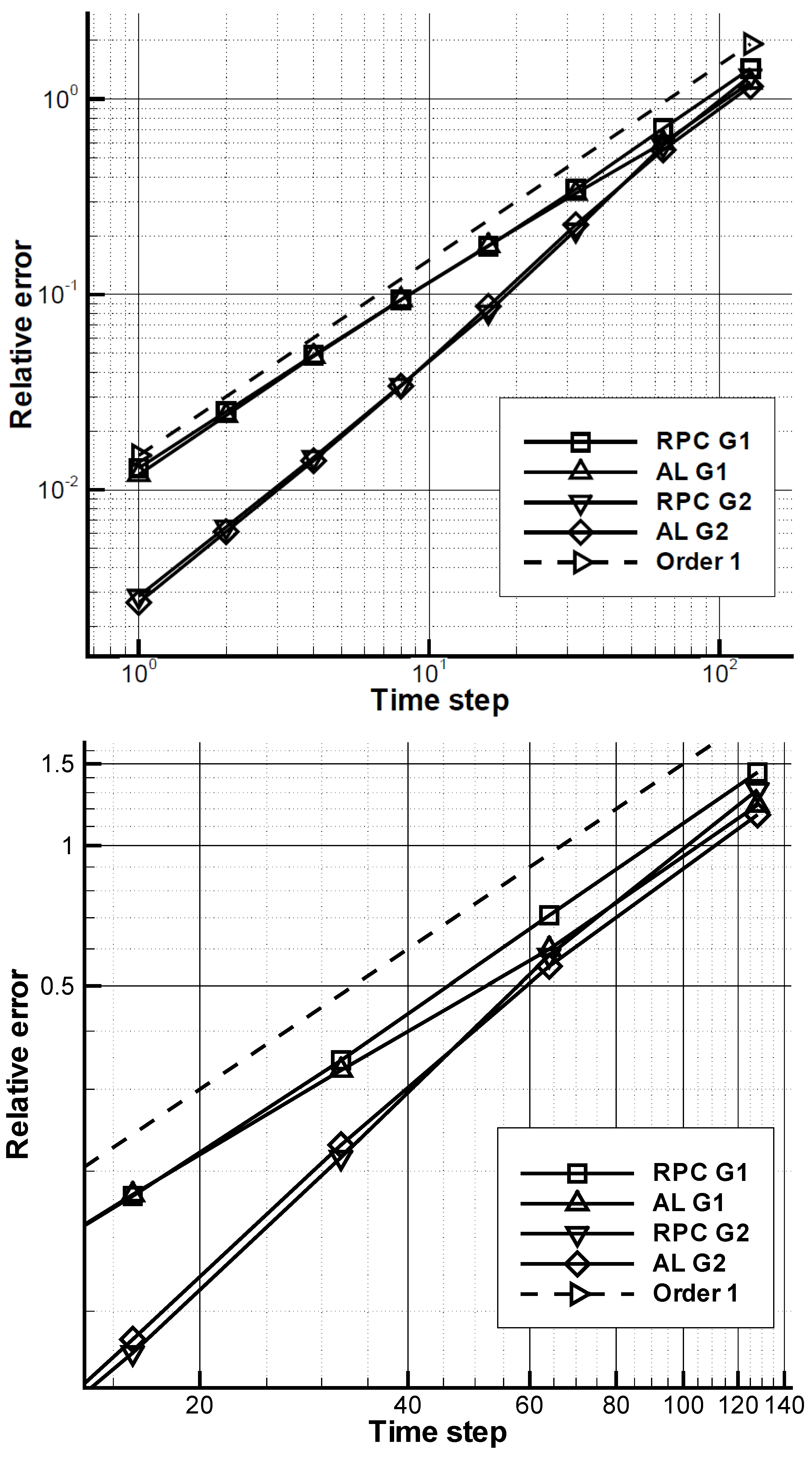
1	$4.726\times {10}^2$	$0.96$	$4.750\times {10}^2$	$1.00$

and

Table 9. Period of the oscillations with the rotational pressure-correction (RPC) and the augmented Lagrangian (AL) with a Gear 2 temporal scheme for the flow past a cylinder at $Re=100$.

$\Delta \mathit{t}/\Delta {\mathit{t}}_{\mathit{min}}$	Period/$\Delta {\mathit{t}}_{\mathit{min}}$ (RPC)	Order	Period/$\Delta {\mathit{t}}_{\mathit{min}}$(AL)	Order
Ref.	$4.673\times {10}^2$		$4.691\times {10}^2$
128	$1.083\times {10}^3$		$1.016\times {10}^3$
64	$7.386\times {10}^2$	$1.18$	$7.278\times {10}^2$	$1.08$
32	$5.671\times {10}^2$	$1.44$	$5.762\times {10}^2$	$1.27$
16	$5.051\times {10}^2$	$1.40$	$5.102\times {10}^2$	$1.39$
8	$4.832\times {10}^2$	$1.25$	$4.853\times {10}^2$	$1.36$
4	$4.740\times {10}^2$	$1.23$	$4.760\times {10}^2$	$1.27$
2	$4.701\times {10}^2$	$1.18$	$4.722\times {10}^2$	$1.21$
1	$4.685\times {10}^2$	$1.18$	$4.706\times {10}^2$	$1.21$

gives the values of a period of oscillation (a-dimensionalized by the minimum time step) for different time steps with the augmented Lagrangian an rotational methods with the first and second-order Gear schemes for the time derivatives. The convergence order is determined with the Richardson extrapolation performed with the three more refined time steps. The results in term of relative error are given in Figure 8.

For both time schemes, the differences between AL and the rotational methods are non-negligible for the larger time steps, with a greater accuracy for the AL. As for the precedent case, it shows the advantage of the AL to deal with larger time steps. For the other time steps, both methodologies reach a similar accuracy. For the smaller time steps (where the asymptotic convergence seems to be reached), the convergence orders on the velocity and the pressure are about 1 for the Euler scheme and about $1.2$ for the second-order Gear scheme. From [41], the rate of error for the $L^2$-norm of the velocity of $O(\Delta t^{\frac{3}{2}})$ is expected.

6. Conclusions

The correction of the first-order $L^2$-penalty method for the pressure-correction methods was extended to a second-order with the Sub-mesh penalty method. The correction converges toward the Ikeno and Kajishima [20] correction, which is designed for a direct-forcing IBM method. The consistency of the method is directly deduced from its construction.

A brief theoretical analysis proved that the temporal error of the pressure correction method with a first-order Gear scheme was not altered. Again, this point is similar to the Ikeno–Kajishima correction. A study with higher integration schemes is now desirable.

Numerical experiments were carried out. The correction was compared to the augmented Lagrangian method and the same results were obtained in space for the cylindrical Couette flow. For this first case, convergence rates of 2 and $1.3$ in the $L^2$-error norm for the velocity and the pressure were obtained. It corresponds to the known performances of the rotational method with Dirichlet boundary conditions. Concerning the flow past a cylinder at $Re=100$, the study showed a maximum convergence order for both augmented Lagrangian and rotational methods of $1.20$. Those results are close to the literature where a convergence rate between $O(\Delta t)$ and $O(\Delta t^{\frac{3}{2}})$ is expected [30]. A combination with the second-order open boundary conditions of [44] could be investigated.

As for a small enough penalty parameter $\epsilon$, the present methodology is equivalent to a corrected direct-forcing IBM, especially the method of [8]; the conclusions of this study can be extended to this method.

This work is also a more general comparison between the rotational pressure-correction and the augmented Lagrangian methods (and this last method can a priori be applied to any DF-IBM method). The results show that the spatial accuracy is the same for both methods. Concerning the time accuracy, the AL approach seems to be more efficient with very-high time steps. For moderate and low time-steps, one cannot conclude. Almost no differences were obtained with the case of the flow past a cylinder. For the Couette flow, quite similar results were obtained for the pressure. For the velocity, the results depend on the time step. For the smaller time steps, the convergence of the AL method decreases while the absolute temporal accuracy is still better than with the rotational method. It was shown that the value of the penalty parameter $dr$ has an influence on the convergence rate. The influence of the number of sub-iterations could be evaluated too. Increasing the number of sub-iteration generally enhances the convergency at the expense of the computational cost. All these considerations show the complexity of a comparative study between those methods (with and without immersed boundary modification). A future work devoted to an extended comparison would be of high interest, especially if simulations of multiphase flows are performed.

References

- Mittal, R.; Iaccarino, G. Immersed boundary methods. Annu. Rev. Fluid Mech. 2005, 37, 239–261. [Google Scholar] [CrossRef] [Green Version]
- Sarthou, A. Fictitious Domain Methods for the Elliptic and Navier–Stokes Equations. Application to Fluid-Structure Coupling. Ph.D. Thesis, Université Bordeaux I, Talence, France, 2009. [Google Scholar]
- Peskin, C.S. Flow patterns around heart valves: A numerical method. J. Comput. Phys. 1972, 10, 252–271. [Google Scholar] [CrossRef]
- Peskin, C.S. The immersed boundary method. Acta Numer. 2002, 11, 479–517. [Google Scholar] [CrossRef] [Green Version]
- Mohd-Yusof, J. Combined Immersed Boundary/b-Spline Methods for Simulations of Flows in Complex Geometries; Annual Research Brief; Stanford University CTR: Stanford, CA, USA, 1997. [Google Scholar]
- Fadlun, E.A.; Verzicco, R.; Orlandi, P.; Mohd-Yusof, J. Combined immersed-boundary finite-difference methods for three-dimensional complex flow simulations. J. Comput. Phys. 2000, 161, 35–60. [Google Scholar] [CrossRef]
- Verzicco, R.; Iaccarino, G.; Fatica, M.; Orlandi, P. Flow in a Impeller Stirred Tank Using an Immersed Boundary Method; Annual Research Brief; Stanford University CTR: Stanford, CA, USA, 2001. [Google Scholar]
- Tseng, Y.-H.; Ferziger, J.H. A ghost-cell immersed boundary method for flow in complex geometry. J. Comput. Phys. 2003, 192, 593–623. [Google Scholar] [CrossRef]
- Arquis, E. Convection Mixte Dans une Couche Poreuse Verticale non Confinée. Application à l’Isolation Perméodynamique. Ph.D. Thesis, Université Bordeaux I, Talence, France, 1984. [Google Scholar]
- Khadra, K.; Angot, P.; Parneix, S.; Caltagirone, J.-P. Fictitious domain approach for numerical modelling of navier-stokes equations. Int. J. Numer. Methods Fluids 2000, 34, 651–684. [Google Scholar] [CrossRef]
- Angot, P.; Bruneau, C.-H.; Fabrie, P. A penalization method to take into account obstacles in incompressible viscous flows. Numer. Math. 1999, 81, 497–520. [Google Scholar] [CrossRef]
- Ramière, I.; Angot, P.; Belliard, M. A general fictitious domain method with immersed jumps and multilevel nested structured meshes. J. Comput. Phys. 2007, 225, 1347–1387. [Google Scholar] [CrossRef] [Green Version]
- Sarthou, A.; Vincent, S.; Angot, P.; Caltagirone, J.-P. The Sub-Mesh-Penalty Method. In Finite Volumes for Complex Applications V; Wiley: New York, NY, USA, 2008; pp. 633–640. [Google Scholar]
- Sarthou, A.; Vincent, S.; Caltagirone, J.-P.; Angot, P. Eulerian-Lagrangian grid coupling and penalty methods for the simulation of multiphase flows interacting with complex objects. Int. J. Numer. Methods Fluids 2008, 56, 1093–1099. [Google Scholar] [CrossRef]
- Fortin, M.; Glowinski, R. Méthodes de Lagrangien Augmenté. Application à la Résolution Numérique de Problèmes aux Limites; Dunod Paris: Paris, France, 1982. [Google Scholar]
- Vincent, S.; Sarthou, A.; Caltagirone, J.-P.; Sonilhac, F.; Février, P.; Mignot, C.; Pianet, G. Augmented lagrangian and penalty methods for the simulation of two-phase flows interacting with moving solids. application to hydroplaning flows interacting with real tire tread patterns. J. Comput. Phys. 2010, 230, 956–983. [Google Scholar] [CrossRef] [Green Version]
- Domenichini, F. On the consistency of the direct forcing method in the fractional step solution of the navier-stokes equations. J. Comput. Phys. 2008, 227, 6372–6384. [Google Scholar] [CrossRef]
- Kim, J.; Kim, D.; Choi, H. An immersed boundary finite volume method for simulations of flow in complex geometries. J. Comput. Phys. 2001, 171, 132–150. [Google Scholar] [CrossRef]
- Taira, K.; Colonius, T. The immersed boundary method: A projection approach. J. Comput. Phys. 2007, 225, 2118–2137. [Google Scholar] [CrossRef]
- Ikeno, T.; Kajishima, T. Finite-difference immersed boundary method consistent with wall conditions for incompressible turbulent flow simulations. J. Comput. Phys. 2007, 226, 1485–1508. [Google Scholar] [CrossRef]
- Ng, Y.T.; Min, C.; Gibou, F. An efficient fluid—Solid coupling algorithm for single-phase flows. J. Comput. Phys. 2009, 228, 8807–8829. [Google Scholar] [CrossRef]
- Lepilliez, M.; Popescu, E.R.; Gibou, F.; Tanguy, S. On two-phase flow solvers in irregular domains with contact line. J. Comput. Phys. 2016, 321, 1217–1251. [Google Scholar] [CrossRef] [Green Version]
- Angot, P.F.P.; Caltagirone, J.-P. Vector Penalty-Projection Methods for the Solution of Unsteady Incompressible Flows. In Finite Volumes for Complex Applications V; Wiley: New York, NY, USA, 2008; pp. 169–176. [Google Scholar]
- Belliard, M.; Fournier, C. Penalized direct forcing and projection schemes for navier-stokes. C. R. Math. 2010, 348, 1133–1136. [Google Scholar] [CrossRef] [Green Version]
- Goda, K. A multistep technique with implicit difference schemes for calculating two- or three-dimensional cavity flows. J. Comput. Phys. 1978, 30, 76–95. [Google Scholar] [CrossRef]
- Timmermans, L.J.P.; Minev, P.D.; Van De Vosse, F.N. An approximate projection scheme for incompressible flow using spectral elements. Int. J. Numer. Methods Fluid 1996, 22, 673–688. [Google Scholar] [CrossRef]
- Gustafsson, I. On First and Second Order Symmetric Factorization Methods for the Solution of Elliptic Difference Equations; Research Report; Department of Computer Sciences, Chalmers University of Technology and the University of Gateborg: Göteborg, Sweden, 1978. [Google Scholar]
- Van Der Vorst, H.A. Bi-cgstab: A fast and smoothly converging variant of bi-cg for the solution of nonsymmetric linear systems. SIAM J. Sci. Stat. Comput. 1992, 13, 631–644. [Google Scholar] [CrossRef]
- Kim, J.; Moin, P. Application of a fractional-step method to incompressible Navier–Stokes equations. J. Comput. Phys. 1985, 59, 308–323. [Google Scholar] [CrossRef]
- Guermond, J.L.; Minev, P.; Shen, J. An overview of projection methods for incompressible flows. Comput. Methods Appl. Mech. Eng. 2006, 195, 6011–6045. [Google Scholar] [CrossRef] [Green Version]
- Arrow, K.J.; Hurwicz, L.; Uzawa, H. Studies in linear and Nonlinear Programming—Iterative Method for Concave Programming; Stanford University Press: Stanford, CA, USA, 1958. [Google Scholar]
- Févriére, C.; Laminie, J.; Poullet, P.; Angot, P. On the penalty-projection method for the navier-stokes equations with the mac mesh. J. Comput. Appl. Math. 2009, 226, 228–245. [Google Scholar] [CrossRef]
- Vincent, S.; Caltagirone, J.-P.; Lubin, P.; Randrianarivelo, T.N. Randrianarivelo. An adaptative augmented lagrangian method for three-dimensional multimaterial flows. Comput. Fluids 2004, 33, 1273–1289. [Google Scholar] [CrossRef]
- Fujii, K. Unified Zonal Method Based on the Fortified Solution Algorithm. J. Comput. Phys. 1995, 118, 92–108. [Google Scholar] [CrossRef]
- Sarthou, A.; Vincent, S.; Caltagirone, J.P. A second-order curvilinear to cartesian transformation of immersed interfaces and boundaries. Application to fictitious domains and multiphase flows. Comput. Fluids 2010, 46, 422–428. [Google Scholar] [CrossRef] [Green Version]
- Ogayar, C.J.; Segura, R.J.; Feito, F.R. Point in solid strategies. Comput. Graph. 2005, 29, 616–624. [Google Scholar] [CrossRef]
- Angot, P. Contribution à l’étude des Transferts Thermiques dans des Systèmes Complexes aux Composants Électroniques. Ph.D. Thesis, Université Bordeaux I, Talence, France, 1989. [Google Scholar]
- Ramière, I. Convergence analysis of the q1-finite element method for elliptic problems with non-boundary-fitted meshes. Int. J. Numer. Methods Eng. 2007, 75, 1007–1052. [Google Scholar] [CrossRef]
- Perot, J.B. An analysis of the fractional step method. J. Comput. Phys. 1993, 108, 51–58. [Google Scholar] [CrossRef]
- Roache, P.J. Verification and Validation in Computational Science and Engineering; Hermosa Publishers: Albuquerque, NM, USA, 1998. [Google Scholar]
- Guendelman, E.; Selle, A.; Losasso, F.; Fedkiw, R. Coupling water and smoke to thin deformable and rigid shells. In Proceedings of the ACM SIGGRAPH, Los Angeles, CA, USA, 2–7 August 2005; pp. 973–981. [Google Scholar]
- Angot, P.; Jobelin, M.; Latché, J.-C. Error analysis of the penalty-projection method for the time-dependant stokes equations. Int. J. Finite Vol. 2009, 6, 1–26. [Google Scholar]
- Orlanski, I. A simple boundary condition for unbounded hyperbolic flows. J. Comput. Phys. 1976, 21, 251–269. [Google Scholar] [CrossRef]
- Poux, A.; Glockner, S.; Azaïez, M. Improvements on open and traction boundary conditions for navier-stokes time-splitting methods. J. Comput. Phys. 2011, 230, 4011–4027. [Google Scholar] [CrossRef]
Figure 1.
Definition of the domains.
Figure 2.
Definition of the discretization kernels.
Figure 3.
Evolution of the spatial error for the velocity and the pressure p with (COR) and without (NC) the second-order correction for the Couette flow.
Figure 4.
Evolution of the -norm of the spatial error for s, s, and s for the Couette flow for the augmented Lagrangian (AL), the incremental pressure-correction (PC), the rotational pressure-correction (RPC), and the uncorrected the rotational pressure-correction (RPC NC).
Figure 5.
Time evolution of the -norm of the spatial error for the velocity and the pressure with the Gear 2 scheme for the augmented Lagrangian method with (AL 10) and (AL 100) and for the rotational pressure-correction (RPC).
Figure 6.
Mesh for the case of the flow past a cylinder at .
Figure 7.
Pressure and vorticity contours for the case of the flow past a cylinder at .
Figure 8.
Evolution of the temporal error for the period of oscillation for the flow past a cylinder at .