Stability Analysis for an Interface with a Continuous Internal Structure

1
Institute de Astrofisica de Canarias, 38205 La Laguna, Tenerife, Spain
2
Departamento de Astrofísica, Universidad de La Laguna, 38205 La Laguna, Tenerife, Spain
Fluids 2021, 6(1), 18; https://0-doi-org.brum.beds.ac.uk/10.3390/fluids6010018
Submission received: 14 December 2020
/
Revised: 27 December 2020
/
Accepted: 27 December 2020
/
Published: 1 January 2021
(This article belongs to the Special Issue Analytical and Computational Fluid Dynamics of Combustion and Fires [dedicated to Prof. Vitaly Bychkov (1968–2015) of Umea University, Sweden])
Abstract
:A general method for solving a linear stability problem of an interface with a continuous internal structure is described. Such interfaces or fronts are commonly found in various branches of physics, such as combustion and plasma physics. It extends simplified analysis of an infinitely thin discontinuous front by means of numerical integration along the steady-state solution. Two examples are presented to demonstrate the application of the method for 1D pulsating instability in magnetic deflagration and 2D Darrieus–Landau instability in a laser ablation wave.
1. Introduction
Linear stability analysis is a powerful technique for investigating a system’s response to small perturbations and answering the main question about whether the system is stable or not. It has been used to predict and explore a vast majority of fluid and plasma instabilities, including Rayleigh–Taylor (RT), Kelvin–Helmholtz, and Darrieus–Landau (DL) instabilities, in addition to many others [1,2].
As a rule, investigation of any instability starts with the analysis of the interface as a discontinuity. It assumes zero thickness of the front, where the flow quantities experience a jump and all the transport mechanisms are neglected. It is justified by the fact that the characteristic length scale of the problem is much larger than the front width. Such an approach simplifies treatment of the governing equations, and in many cases, the dispersion relation can be derived analytically. However, the obtained results may differ a lot from or even contradict experimental observations. For example, the RT instability in inertial confinement fusion distorts the pellet symmetry, decreasing the fuel compression and limiting the net gain of nuclear reaction [3]. This was confirmed experimentally, but the instability evolves at a much slower pace than that estimated with the discontinuity approach. Another more illustrative example comes from combustion theory, where a planar flame front of zero thickness was predicted to be unstable due to the Darrieus–Landau instability [1,4], while experiments reveal stable flame propagation with a planar front. Later, those contradictions were resolved by taking into account transport processes within the front and its finite thickness.
As we can see, taking into account the finite front width affects the results of the stability analysis both quantitatively and qualitatively. Furthermore, it yields the characteristic length scale of the instability or the cut-off wave length, if there is one. There are several ways to include the interface thickness under consideration. The simplest option is to specify the front structure artificially, e.g., linear or exponential spatial distribution. The specific profile is chosen in such a way that solving the problem is facilitated. A typical example is to assume an exponential density profile in studies of various instabilities in plasma physics [2,5]. Very often, such a consideration requires an additional matching condition at the front. For example, the model of a discontinuous ablation front used to study the RT instability contains a deficit in the boundary conditions; the number of unknowns exceeds the number of conservation laws at the front by one. This deficit was first encountered for the RT instability in laser fusion [6], and it is common for other problems as well [7]. In the case of incompressible flow, the extra condition may be easily guessed; it is the well-known DL condition of a constant flame velocity with respect to the fuel mixture; one may also prove it rigorously for an isobaric flow [1,4]. When compression effects are taken into account, the problem of the additional boundary condition becomes a difficulty again. Incorrect assumptions may lead to contradictory results and erroneous conclusions [7,8].
This paper is devoted to a method of solving the stability problem at the interface with a realistic continuous internal structure. It eliminates the problem of the extra matching condition by integrating the perturbed equations along the continuous profile of the steady-state solution. It has already been used previously [8,9,10,11]; however, its thorough description is still missing, which makes it difficult to apply in different fields. Below, we present a general algorithm of the method and discuss all essential steps that are necessary for its application. This is followed by two examples where the method is used for 1D and 2D problems. The paper finishes with a conclusion section.
2. General Algorithm
The whole algorithm consists of several consequent steps. For a typical 2D stability problem with dispersion relation , where is the instability growth rate and k is the perturbation wave number, these steps are the following:
- (a)
- Compute the steady-state solution and obtain the 1D profile;
- (b)
- Derive the linearized system of equations in 2D;
- (c)
- Fix k;
- (d)
- Fix ;
- (e)
- Compute the eigenvalues (modes ) with eigenvectors of the perturbed system;
- (f)
- For every mode, integrate the perturbed system and gather the perturbation amplitudes into a matrix;
- (g)
- Compute the determinant of this matrix;
- (h)
- Change and repeat steps (e–g), searching for the zero determinant;
- (i)
- Repeat steps (d–h) for different k to complete the dispersion relation.
Below, we will discuss each of these steps.
- (a)
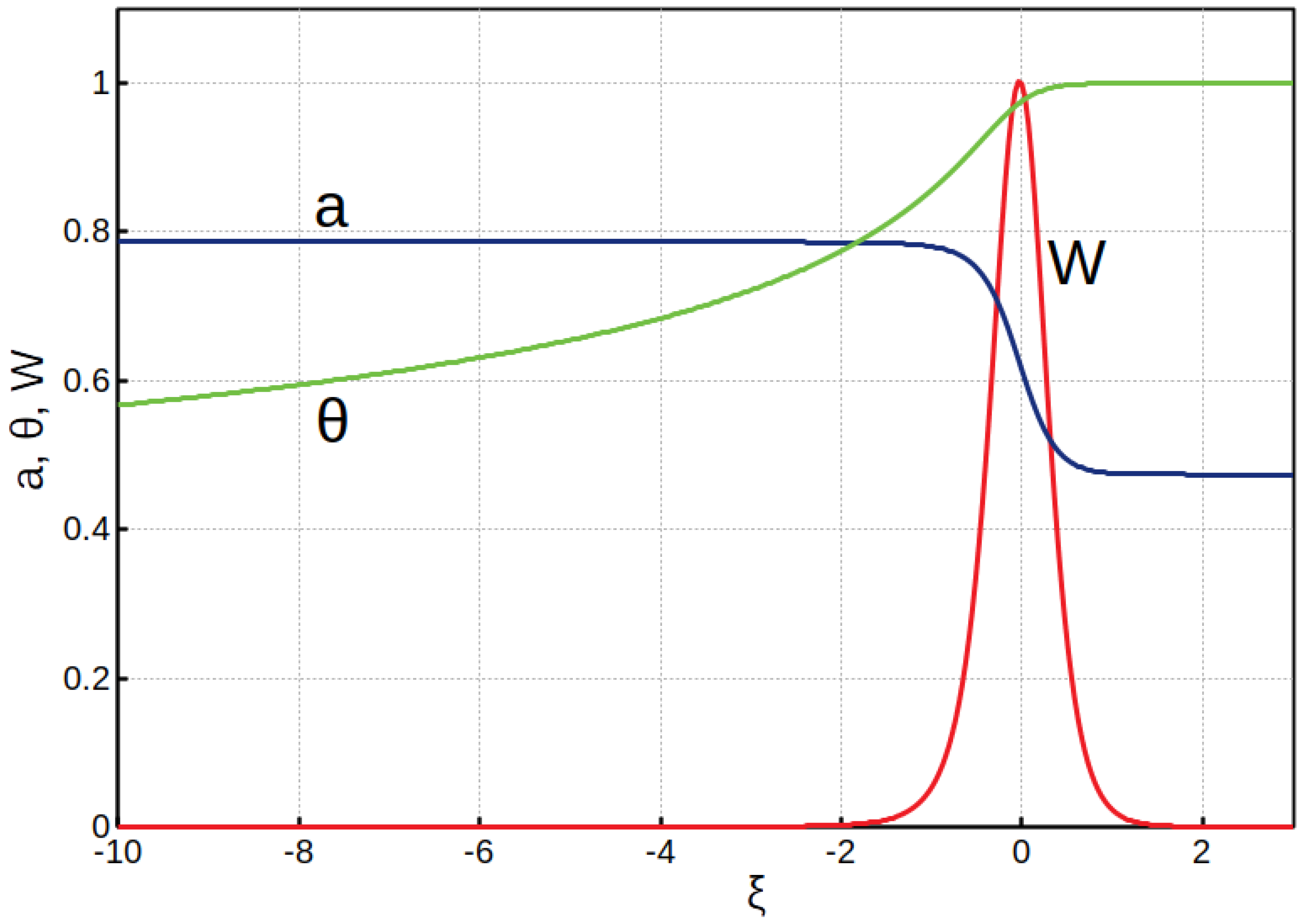
- The internal structure of the stationary front profile is defined by transport mechanisms and sources, if there are any; dissipative processes, like viscous dissipation, are omitted, as they do not allow a steady-state solution. Finding a steady state is a separate and standalone problem, which is not covered by this paper; typical profiles are shown in Figures 1 and 3.The profile can be virtually split into three parts: a central one—the actual front, where the media changes its phase—and the two uniform regions (tails) far from the central part.
- (b)
- Next, we apply small perturbations to the steady-state solution. In the 2D case, every system independent variable (such as density, temperature, and velocity) is written aswhere is a stead-state solution varying along the x coordinate, is the instability growth rate, k is the perturbation wave number, t stands for time, and y is a coordinate normal to the profile. It is important to notice that the perturbed part () varies along the profile, while in the perpendicular direction, it is determined by the wave number. In general, the instability growth rate is a complex number, with the real part standing for the growth or damping rate of the perturbations, and the imaginary part standing for the oscillation frequency. If the real part of is positive, the perturbations grow, leading to an unstable solution. Negative real implies damping of the perturbations and stable configuration of the front. Usually, the stability analysis resolves only either the pure real or pure imaginary part of the instability.A necessary condition for the applicability of the method is the possibility of writing down the linearized system in the following form:This system has N independent variables. It is important to notice that the matrix F depends on the steady-state variables and varies along the profile. It also depends on and k.
- (c,d)
- For the sake of clarity, it is convenient to postpone the explanation of the aim of steps (c,d) in the algorithm. The way to vary and k depends on the particular problem, its stability limits, the cutoff wave number, existence of multiple roots, etc.
- (e)
- The solution to the stability problem arises as an eigenvalue of system (2). Prior to the numerical integration, it is necessary to find proper boundary conditions for this system. The existence of the uniform tails with negligible gradients where all the variables remain nearly constant is an essential feature of this analysis. In these tails, the coefficients of matrix F from Equation (2) become constant in space, and with fixed and k, the above system has a trivial exponential solution:where is an eigenvalue (a “mode”) of matrix F and is a corresponding eigenvector. In order to find eigenvalues , we substitute expression (3) into the system (2) and equate the obtained determinant to zero:It is often possible to write down this equation as a polynomial with respect to and solve it analytically; in more realistic and complicated systems, the modes can only be calculated numerically. There are N different eigenvalues at each side of the front; however, not all of them are physical. The instability develops at the central part of the front, while in the uniform tails, all the perturbations must vanish. This determines the choice for proper mode selection by its sign. On the left side of the front in Figure 1, a mode with a positive sign grows towards the central part of the front and vanishes at . A negative mode has the opposite behavior, growing in the uniform tails, which is unphysical; therefore, it should be excluded. Hence, we obtain a set of positive modes for the left side of the front and a set of negative modes for the right side of the front,The number of suitable modes can be different at each side of the front, but their total number must be equal to the order of the system N. Every mode produces its eigenvector. This means that one perturbation amplitude is chosen arbitrary, while the others are derived from that amplitude. It is worth mentioning that if some modes are complex or purely imaginary, this method cannot be applied in its current form.
- (f)
- The above modes and eigenvectors constitute the boundary conditions for the numerical integration of the system (2) along the steady-state profile. Suppose that there are positive modes and negative modes. Next, we choose a “matching point” at the stationary profile, say ; from a numerical viewpoint, it is advisable to choose a point within a region of maximal gradients. Then, for each positive mode, the system (2) is integrated from the left side of the front until the point; in total, integrations are to be performed. Similarly, for every negative mode, the system is integrated backwards, from the right front side until the point; in total, integrations are to be performed. Integration can be done by any suitable computational method, like the explicit Runge–Kutta 4 or others.
- (g)
- Every integration produces a vector of perturbation amplitudes. At the matching point, we build an matrix from these amplitudes and compute its determinant; its value depends on k and .
- (h)
- (i)
- Finally, steps (d–h) are repeated for different k to compute the whole dispersion relation.
Below, we consider two examples demonstrating an application of this method in 1D and 2D cases. The first example is described in more detail so that it is easier to follow all the steps of the algorithm. The second example has fewer details, although all important steps are discussed.
3. One-Dimensional Pulsating Instability in Molecular Magnets
Molecular magnets have been explored for about forty years due to their unique properties and potential applications in novel storage devices and quantum computing [12]. During the last fifteen years, the so-called magnetic combustion has brought new attention to the field. It was discovered that under certain conditions, a wave of magnetization reversal travels within a crystal of molecular magnets [13]. This wave propagates with a velocity of several meters per second and is accompanied by a significant heat release, similarly to a deflagration wave in combustion; for this reason, it was named “magnetic deflagration” [14]. In chemical combustion, the deflagration front corresponds to a thin zone of chemical reactions separating the cold fuel mixture and the hot burned products. The released energy is transmitted to the cold fuel mixture due to thermal conduction; the temperature of the fuel mixture increases, which stimulates chemical reactions. Analogously, in magnetic deflagration, the energy of the chemical reactions is replaced by the Zeeman energy of the molecular magnets in an external magnetic field. The released energy is distributed to the neighboring layers by thermal conduction, which increases the temperature of the originally cold medium and leads to a much higher probability of spin transition. The corresponding theory has been developed to describe the major properties of magnetic deflagration, including the front velocity and temperature [11,14]. As this paper is devoted to the stability analysis, all physical aspects are omitted here; they can be found in the above reference. Below, we expand Section IV of Ref. [11] with more details and discussions according to the algorithm presented in the previous section.
We start with the governing equations for magnetic deflagration in dimensionless form:
where are the scaled temperature, concentration, coordinate, the activation energy, and the Zeeman energy, respectively; J is the ratio of Zeeman and thermal energies, and is an eigenvalue of the stationary solution standing for the front velocity.
- (a)
- There are several ways to find a steady-state solution to the system (7). We write those equations in the reference frame of the moving front, integrate them from both sides, and use the shooting method to find the front eigenvalue and compute the profiles. The profiles of concentration and temperature together with the energy release for the stationary magnetic deflagration front are shown in Figure 1.
- (b)
- Next, we apply small perturbations to this equilibrium state and derive a system of linearized equations. All the variables take the form , and the perturbed linearized system (7) iswhereis introduced for brevity.
- (c)
- In this problem, we investigate stability of the system with respect to the activation energy. Neglecting the width of the energy release zone, it is possible to solve the problem analytically. The corresponding analysis is performed in Section III of Ref. [11]; it results in a quadratic equation for ,where plays the role of the Zeldovich number [4], and is a constant parameter. From this equation, it is known that the system is stable () if the activation energy is below a certain critical value, and above this value, it becomes unstable () and demonstrates pulsating behavior (). In addition, at high values of the activation energy, there are two real solutions to Equation (9). We will use this fact and start searching for a numerical solution in the region of high activation energy (see Figure 2).Since this is a 1D problem and there is no k mentioned in the general algorithm, we fix the activation energy and search for the growth rate .
- (d)
- Fix and compute the system modes.
- (e)
- Substituting expression (3) into system (8), we obtain the following determinant:which is equivalent to Equation (4). This determinant of the third order can easily be expanded into a polynomial, and the modes can be found analytically. Each side of the front has three distinct roots, though only some of them stand for a physical solution. In particular, this system has two modes in the “hot” region (, ) and one mode in the “cold” region (, ). Looking at the stationary profiles in Figure 1, we choose limiting points for the profile. To be specific, we take as the left border and as the right border of the front.The computed modes are the eigenvalues of the system. Next, it is necessary to build corresponding eigenvectors. For that, the system (8) is rewritten asHaving fixed the amplitude of one particular perturbation, the others are derived in a straightforward way. For example, if one fixes , then is easily derived from the third equation of (11) asIn a similar way, is derived from the second equation. It is worth reminding the reader that these relations depend on the mode and on the particular location at the profile (equilibrium variables and ).
- (f)
- Hence, we obtain a vector of perturbation for each mode—three in total. They are the boundary conditions for the integration of the system (8) along the profile. As mentioned in the previous section, the integration can be done by any suitable numerical method. First, we are to define a matching point at the front. According to Figure 1, is a suitable choice; physical results do not depend on the choice of the matching point. There is one mode in the cold (left) region, so the system (8) is integrated once from until . The result of integration is a vector with three perturbation amplitudes, Then, we integrate the system (8) backwards twice from till for the two positive modes and collect the resulting vectors of perturbations.
- (g,h)
- At the matching point, we build a matrix from those vectors and compute its determinant:The value of this determinant depends on (the activation energy is kept fixed). The zero determinant (12) defines the solution for a specific activation energy value.
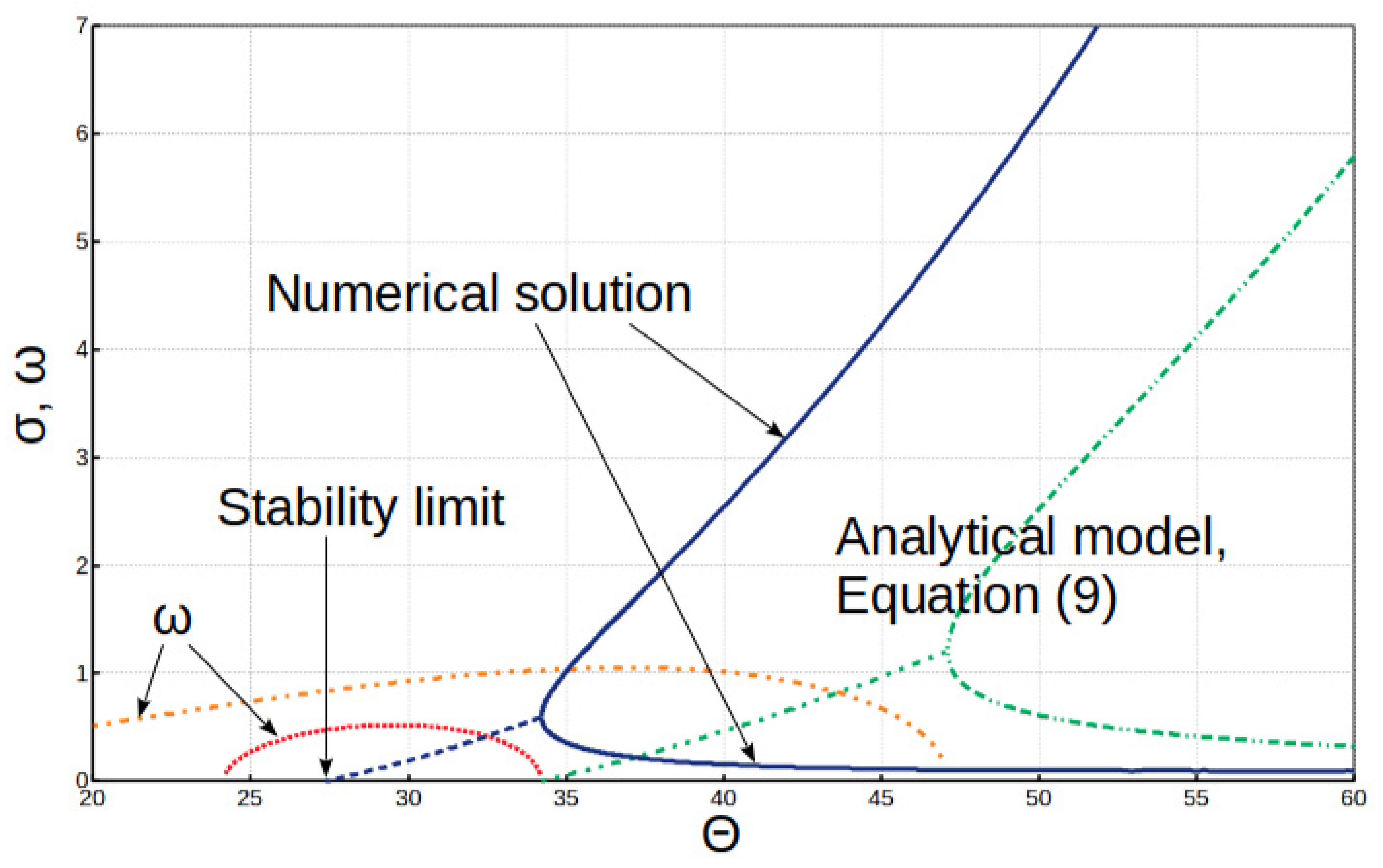
In Figure 2, we demonstrate the dimensionless instability growth rate together with the oscillation frequency as a function of the activation energy. The solid lines depict the numerical solution obtained with this method, and the dashed-dotted lines represent the analytical solution from Equation (9). Leaving aside the physical aspects of the obtained results, we discuss a few technical issues below.
In the region of high activation energy, the two real positive solutions are found numerically. By reducing the activation energy, these solutions merge into one at the bifurcation (), and at lower activation energy, no solution can be found by this method directly. Taking advantage of the analytical Equation (9), it is natural to assume that at the bifurcation point, the discriminant becomes negative and the solution becomes complex with real and imaginary parts. In order to compute complex roots in the case of a continuous front, at a given activation energy, we approximate the solution using the quadratic parabola:
where a, b, and c are unknown coefficients and D is computed by Equation (12). Formally, the obtained roots would be of the second order of accuracy, which is more than enough for linear stability analysis. To find these coefficients, we compute determinant D for three “guess” values of and build a system of three linear Equation (13) with respect to its coefficients. From this system, we calculate the coefficients a, b, and c and then compute the real () and imaginary () constituents of the solution. The obtained solution becomes more accurate if the “guess” is taken in the close vicinity of the found root. Therefore, one can take several iterations to increase the accuracy of the computed complex roots. Following this approach, we build real and imaginary parts of the complex solution in Figure 2 between and .
In order to verify the obtained solution, we perform direct numerical simulations of the governing Equations (7). At high values of the activation energy, the system evolves in a very nonlinear way, demonstrating strong pulsations (see Ref. [11] for details). Hence, it is not feasible to compare the results of the direct simulation with the solution obtained by this method. However, it is possible to check the stability limit of the system, as, in this region, the instability growth rate is small and the perturbations evolve linearly as a sinusoidal wave of growing or decaying amplitude. Our simulations demonstrate very good agreement for the stability limit denoted in Figure 2. If the activation energy is smaller than this limit, the initial perturbations vanish, revealing a negative real part of the growth rate. If the activation energy is higher than this limit, the perturbations grow, standing for a positive real part of the growth rate. The frequency of the oscillations also fits well with the computed imaginary part of the instability growth rate, . Thus, the direct numerical simulations confirm that the proposed method provides a more accurate solution to the stability problem when the internal structure of the front is taken into account.
The analytical solution (9) obtained within the model with an infinitely thin transition zone (dashed-dotted lines) shows qualitatively similar behavior to that of the numerical solution; however, there is noticeable quantitative difference between them. According to the analytical model, the stability limit and the bifurcation point occur at 30–40% smaller activation energies. In addition, at a given activation energy, the simplified model predicts a much weaker growth rate, e.g., at , Equation (9) yields , while the numerical solution produces . Hence, the analytical model significantly underestimates the instability growth rate and overestimates the stability limit of this instability. The limited accuracy of the analytical model is due to the simplifying approximations of a constant coefficient of energy diffusion and an infinitely thin zone of the energy release.
4. Two-Dimensional Darrieus–Landau Instability in Laser Ablation
In this section, we consider the classical 2D Darrieus–Landau instability [1,4] in a wave of laser ablation [3,7,8]. This instability develops at a deflagration front, i.e., a front of energy release propagating subsonically due to thermal conduction. In contrast to a conventional combustion wave, the laser ablation implies a highly compressible flow, with the isothermal Mach number reaching unity at the critical surface [3,7,8]. Below, we follow our analysis [8], paying more attention to the technical issues.
- (a)
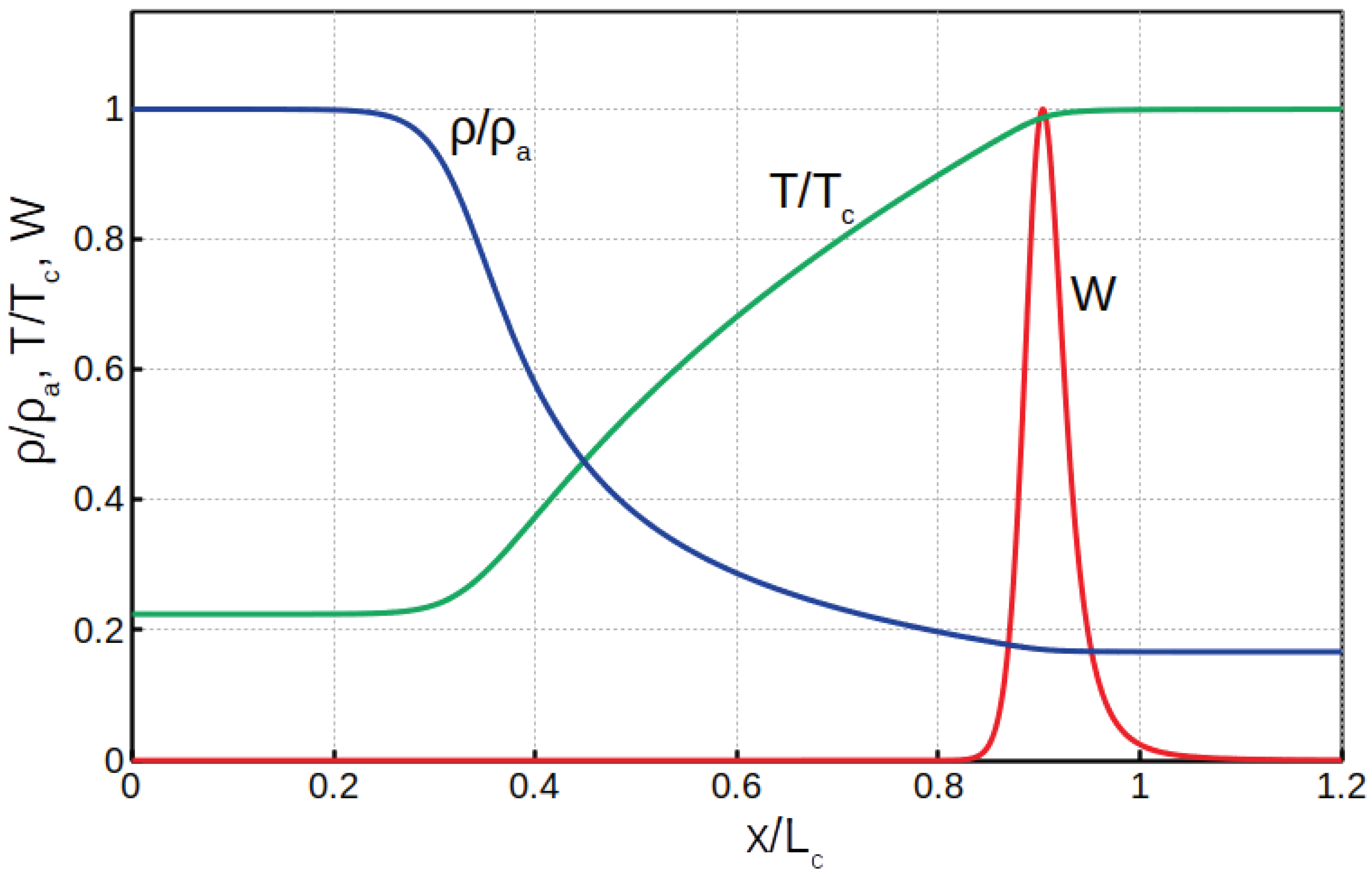
- We describe laser plasma within the one-fluid approximation using the ideal gas equation with a single temperature. This is a traditional approach for studying hydrodynamic instabilities in inertial fusion and is employed in the absolute majority of works on the subject [3]. We model an ablation wave with the Navier–Stokes equations for density, momentum, and energy:and the equation of state of ideal gas completes the system, . Electron thermal conduction depends on temperature as , the subscript “c” stands for the critical surface where the laser irradiance is absorbed. The energy release due to laser absorption is taken in a form similar to the Arrhenius law in combustion:where plays a role of the scaled activation energy. This particular form for is constructed to model very localized energy release, so the activation energy is set very high: in this sample.The typical internal structure of the stationary deflagration front is illustrated in Figure 3. It is mostly determined by the energy equation. Scale separation in the front structure is an important feature of laser ablation. One can identify a narrow region of the energy release and another region of the maximal density gradient. Both regions are separated from each other, and they are significantly smaller than the overall front width.
- (b)
- Such a complicated structure cannot be taken into account by usual analytical stability analysis. To be specific, we consider a wave of laser ablation propagating along the x direction, and the instability evolves along the y coordinate. Small perturbations are written as . Then, the linearized system (14) takes the following form:It is important to notice that the shape of the system differs from the necessary form (2) of the general algorithm (compare also with (8)). To overcome this limitation, we introduce new perturbation variables [9] and rewrite everything in dimensionless form:with the scaled wave number, , and the perturbation growth rate, ; is the characteristic width of the front determined by thermal conduction in the hot region. We also introduce an auxiliary variable ; this step is a common way to rewrite a second-order Equation () as two equations of the first order. Then, the linearized system (16)–() can be presented in a matrix form (2), withwhere dimensionless variables are , , , , and ; is the flow Mach number defined in the hot region, and coefficients depend on the steady-state solution and vary along the profile. For their exact expressions, see the Appendix in Ref. [8]. It is worth mentioning that for this problem, presenting the perturbed linearized equation in this proper form is the most tricky part.
- (c,d)
- For a chosen Mach number, we fix K and S and proceed according to the algorithm. In the incompressible case, the dispersion relation of the DL instability has a parabolic shape with a certain cutoff wavelength. Hence, it is advisable to start computing the dispersion relation from small values of the wavenumber K and increase it gradually until the cutoff (negative ) is found.
- (e)
- Next, we solve Equation (4) and compute five modes of the system. The equation for can be written as a fifth-order polynomial. In the incompressible case (), it simplifies a lot and can be solved analytically; in the general case, it is solved numerically. The system has two positive ( for ) and three negative modes ( for ). For each mode, we compute the corresponding eigenvector at its boundary. It is advisable to derive relationships between different perturbation amplitudes, as one mode may either nullify one perturbation amplitude or lead to division by zero error. The derived expressions help to identify which perturbation amplitude can be set to a small arbitrary value so that the others can be computed.
- (f)
- (g–i)
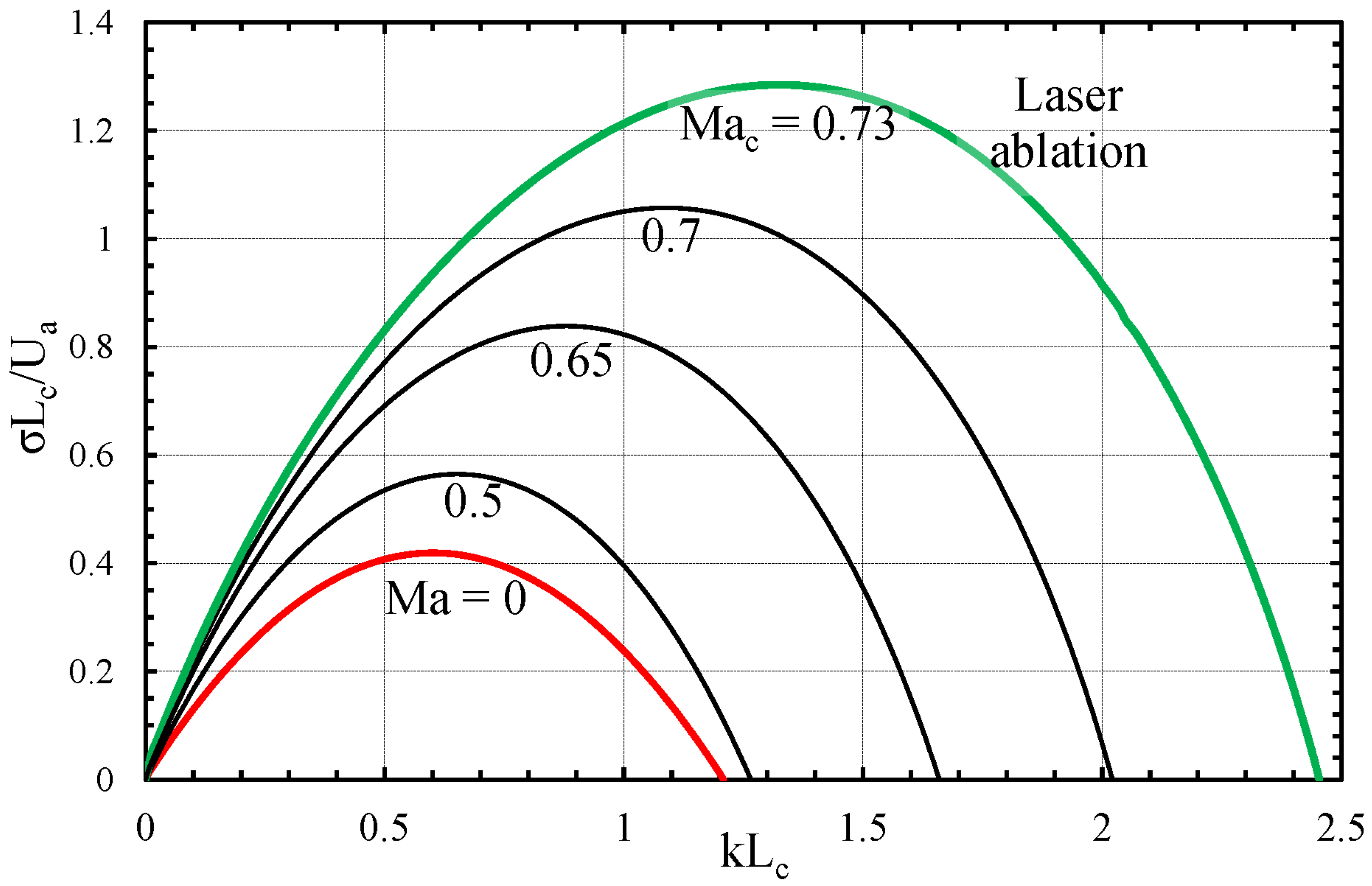
- At the matching point, we gather the results of the integrations into a matrix of perturbation amplitudes and compute its determinant. The zero determinant stands for the solution for the stability problem. Varying K and repeating steps (e,f), we compute the whole dispersion relation. In Figure 4, the resulting curves are illustrated for different Mach numbers. This clearly demonstrates that a compressible deflagration flow is more unstable. It has a higher maximal growth rate and a broader scale range where the front is unstable.
These results reveal similar behavior to that in previous studies on the DL instability in compressible combustion fronts [9,10]. They are also in line with discontinuous analysis in the long wavelength limit [15,16], where an extra boundary condition was chosen analogously to the DL condition in the incompressible case. However, Ref. [7], where an extra boundary condition was rigorously derived, predicted that the instability vanished in a highly compressible case. Thus, the method can verify whether a simplified discontinuous approach produces reasonable results, as it does not need any additional boundary conditions.
5. Discussions and Conclusions
In this paper, we consider a general method for investigating the instability of an interface with a continuous internal structure. The application of this method for different physical problems was thoroughly demonstrated.
In the example of the 1D problem, this method provides a more accurate solution than the discontinuous approach, which is justified by direct numerical simulations. For the 2D problem of the DL instability, this method allows the resolution of the dispersion relation without an extra matching condition, which is needed for the discontinuous approach.
From the point of view of computational cost, this method is more expensive than analytically solving the derived equation for the dispersion relation. It does require multiple numerical integrations along the 1D steady-state solution, which is still relatively quick. On the other hand, the method is significantly cheaper than direct numerical simulation of the governing equations. The latter becomes crucial for 2D and 3D problems, like the DL instability described in Section 4. To be specific, it takes several minutes to compute one curve in Figure 4 using this method. On the contrary, direct numerical simulation of a single point on a curve takes a day or more. For 1D problems, such a comparison is less impressive, but still, direct simulation requires much more time resources.
An important limitation of the method is related to the particular form of the governing equations. In the linearized form, they must be written in the form of a system of the first-order differential equations. In some cases, like in the DL instability example from Section 4, introduction of new variables helps to overcome this limitation and resolve the problem. In addition, this method cannot be applied for nonlinear instabilities of subcritical setups [17], where initial perturbations are assumed to be large.
Despite the fact that both examples are focused on the instability growth rate, the method can also be used to study the dispersion of waves, which is of high relevance to plasma physics. In order to treat waves, one has to replace the instability growth rate with a frequency during the derivation of the linearized equations, . Both real and imaginary parts can be computed numerically using the approach described in Section 3.
This method may also be applied for 3D problems, where expression (1) for small perturbations is expanded as . In such a case, step (c) of the algorithm is split into two subsequent steps for and , respectively. The linearized system will have more equations for perturbations and there will be more modes, but conceptually, the method does not change. It will still require integration along the 1D stationary profile.
Thus, originating from combustion theory, this method can be used in many other fields to investigate stability and waves under much more realistic assumptions than usual jump conditions at the front, and thus produces more accurate and robust results.
Funding
This work was supported by the Spanish Ministry of Science through the project PGC2018- 095832-B-I00. It contributes to the deliverable identified in the FP7 European Research Council grant agreement ERC-2017-CoG771310-PI2FA for the project “Partial Ionization: Two-Fluid Approach”.
Acknowledgments
This paper is dedicated to the memory of Vitaly Bychkov (1968–2015), my former PhD supervisor. The paper is based on our previous works done under his effective and productive guidance. Damir Valiev is acknowledged for motivation and constructive discussions.
Conflicts of Interest
The author declares no conflict of interests.
References
- Landau, L.; Lifshitz, E. Fluid Mechanics; Pergamon: Oxford, UK, 1989. [Google Scholar]
- Chandrasekhar, S. Hydrodynamic and Hydromagnetic Stability; Dover Publications: New York, NY, USA, 1981. [Google Scholar]
- Bychkov, V.; Modestov, M.; Law, C.K. Combustion phenomena in modern physics: I. Inertial confinement fusion. Prog. Energy Combust. Sci. 2015, 47, 32. [Google Scholar] [CrossRef]
- Zeldovich, Y.; Barenblatt, G.; Librovich, V.; Makhviladze, G. The Mathematical Theory of Combustion and Explosion; Consultants Bureau: New York, NY, USA, 1985. [Google Scholar]
- Bychkov, V.; Marklund, M.; Modestov, M. The Rayleigh-Taylor instability and internal waves in quantum plasmas. Phys. Lett. A 2008, 372, 3042. [Google Scholar] [CrossRef]
- Bodner, S. Rayleigh-Taylor Instability and Laser-Pellet Fusion. Phys. Ref. Lett. 1974, 33, 761. [Google Scholar] [CrossRef]
- Bychkov, V.; Modestov, M.; Marklund, M. The Darrieus-Landau instability in fast deflagration and laser ablation. Phys. Plasmas 2008, 15, 032702. [Google Scholar] [CrossRef] [Green Version]
- Modestov, M.; Bychkov, V.; Valiev, D.; Marklund, M. Growth rate and the cutoff wavelength of the Darrieus-Landau instability in laser ablation. Phys. Rev. E 2009, 80, 046403. [Google Scholar] [CrossRef] [PubMed] [Green Version]
- Liberman, M.A.; Bychkov, V.V.; Goldberg, S.M.; Book, D.L. Stability of a planar flame front in the slow combustion regime. Phys. Rev. E 1994, 49, 445. [Google Scholar] [CrossRef] [PubMed]
- Travnikov, O.Y.; Liberman, M.A.; Bychkov, V.V. Stability of a planar flame front in a compressible flow. Phys. Fluids 1997, 9, 12. [Google Scholar] [CrossRef]
- Modestov, M.; Bychkov, V.; Marklund, M. Pulsating regime of magnetic deflagration in crystals of molecular magnets. Phys. Rev. B 2011, 80, 214417. [Google Scholar] [CrossRef]
- Gatteschi, D.; Sessoli, R. Quantum Tunneling of Magnetization and Related Phenomena in Molecular Materials. Angew. Chem. Int. Ed. 2003, 42, 268. [Google Scholar] [CrossRef] [PubMed]
- Suzuki, Y.; Sarachik, M.P.; Chudnovsky, E.M.; McHugh, S.; Gonzalez-Rubio, R.; Avraham, N.; Myasoedov, Y.; Zeldov, E.; Shtrikman, H.; Chakov, N.E.; et al. Propagation of Avalanches in Mn12-Acetate: Magnetic Deflagration. Phys. Rev. Lett. 2005, 95, 147201. [Google Scholar] [CrossRef] [PubMed] [Green Version]
- Garanin, D.A.; Chudnovsky, E.M. Theory of magnetic deflagration in crystals of molecular magnets. Phys. Rev. B 2007, 76, 054410. [Google Scholar] [CrossRef] [Green Version]
- Kadowaki, S. Instability of a deflagration wave propagating with finite Mach number. Phys. Fluids 1995, 7, 220. [Google Scholar] [CrossRef]
- He, L. Analysis of compressibility effects on Darrieus-Landau instability of deflagration wave. Europhys. Lett. 2000, 49, 576. [Google Scholar] [CrossRef]
- Lesur, M.; Médina, J.; Sasaki, M.; Shimizu, A. Subcritical Instabilities in Neutral Fluids and Plasmas. Fluids 2018, 3, 89. [Google Scholar] [CrossRef] [Green Version]
Figure 1.
Stationary magnetic deflagration front: scaled profiles of concentration, temperature, and energy release (see Ref. [11]).
Figure 1.
Stationary magnetic deflagration front: scaled profiles of concentration, temperature, and energy release (see Ref. [11]).

Figure 2.
The instability growth rate and the oscillation frequency vs. the scaled activation energy ; the solid line stands forthe numerically computed solution and the dashed-dotted line corresponds to the analytical solution (9) (see Ref. [11]).

Figure 3.
Stationary deflagration front with : scaled profiles of density, temperature, and energy release (see Ref. [8]).
Figure 3.
Stationary deflagration front with : scaled profiles of density, temperature, and energy release (see Ref. [8]).

Figure 4.
Scaled dispersion relation for different Mach numbers (see Ref. [8]).
Figure 4.
Scaled dispersion relation for different Mach numbers (see Ref. [8]).

Publisher’s Note: MDPI stays neutral with regard to jurisdictional claims in published maps and institutional affiliations. |
© 2021 by the author. Licensee MDPI, Basel, Switzerland. This article is an open access article distributed under the terms and conditions of the Creative Commons Attribution (CC BY) license (http://creativecommons.org/licenses/by/4.0/).
Share and Cite
MDPI and ACS Style
Modestov, M. Stability Analysis for an Interface with a Continuous Internal Structure. Fluids 2021, 6, 18. https://0-doi-org.brum.beds.ac.uk/10.3390/fluids6010018
AMA Style
Modestov M. Stability Analysis for an Interface with a Continuous Internal Structure. Fluids. 2021; 6(1):18. https://0-doi-org.brum.beds.ac.uk/10.3390/fluids6010018
Chicago/Turabian StyleModestov, Mikhail. 2021. "Stability Analysis for an Interface with a Continuous Internal Structure" Fluids 6, no. 1: 18. https://0-doi-org.brum.beds.ac.uk/10.3390/fluids6010018