
Parameter Variability in Viscous Convection


Department of Applied Geosciences, German University of Technology in Oman (GUtech), Halban 1816, Oman
Fluids 2021, 6(11), 376; https://0-doi-org.brum.beds.ac.uk/10.3390/fluids6110376
Submission received: 18 August 2021
/
Revised: 8 October 2021
/
Accepted: 9 October 2021
/
Published: 22 October 2021
(This article belongs to the Special Issue Convection in Fluid and Porous Media)
Abstract
:For the optimal design of cooling and heating devices, the properties of the included fluids are crucial. The temperature dependence of viscosity deserves attention, as changes can be one order of magnitude or more. Here we examine the influence on convective motions by simulating a heating and cooling experiment with a vertical cylinder by finite element computational fluid dynamics (CFD) models. Such an experimental setup in which flow patterns are determined by transient viscous convection has not been simulated before. Evaluating the general behavior of the experiment in 2D, we find a dynamic phase after and before phases with moderate changes. Flow patterns in the dynamic phase change significantly with the temperature range of the experiment. We compare the outcome of the numerical models with results from laboratory experiments, finding major discrepancies concerning the flow patterns in the dynamic phase. 3D modeling shows weaker dynamics but does not show good timing with the experiment. The study depicts the importance of parameter dependencies for convective motions and demonstrates the capabilities and limitations of models to reproduce details of viscous convection.
1. Introduction
Viscous fluids are crucial components used in various applications. They are used as lubricants, in heat exchangers, etc., generally in cooling and heating facilities at very different scales. They are pivotal for cooling cores of nuclear reactors at the large scale, refrigerators and air conditioners at the medium scale, and electronic devices such as transistors and chips at the micro-scale.
For the optimal design and application of these facilities, the parameter dependencies of viscous fluids have to be taken into account. As most applications deal with heat transfer, it is the temperature dependence that is of specific interest, in particular when dealing with a wide temperature range.
For applications in heat transfer, the following fluid parameters have to be taken into account: Density, viscosity, thermal conductivity, and heat capacity. As an example, Figure 1 shows the temperature dependency of these parameters for the oil SAE90. This oil is commonly known as motor lubricant. According to the grading of the Society of Automotive Engineers (SAE)m its kinetic viscosity ranges between a minimum of 13.5 cSt, and a maximum of 24 cSt at 100 °C. The relations depicted in Figure 1 yield a value of 18.4 cSt at 100 °C. The exact mathematical formulations used for the graphs are given below.
It is a common observation that viscosity has the highest variability among the four parameters mentioned. This is clearly visible in the plots in Figure 1. The viscosity plot clearly shows curvature, while the other parameters deviate marginally from linear relations. The viscosity range may span more than one order of magnitude for relatively moderate temperature intervals.
For common fluids, several functional formulations can be found that describe the effect of temperature T on the parameters. The dependence is often defined in relation to a reference value Tref.
may represent any of the mentioned parameters. Equation (1) is valid with and an empirical constant γ. In reaction engineering temperature dependencies, the general Arrhenius equation is often preferred:
with activation energy Ea and Boltzmann constant kB [2]. The coefficient in formula (0) depends on the reference temperature. The viscosity dependence on T in the Arrhenius-type equations is discussed in detail by Messaâdi et al. [3] and Ike [4]. For a rigorous dimensionless description, it is necessary to transform it to a functional formulation that is independent of the choice of a reference point. Pawlowski [1] showed that the one-parametric set of functions, defined by
fulfils the latter condition. Using the functions, the parameter dependency can be expressed as:
The formulations in Equation (4) depend on the constants . As an example, Table 1 lists the coefficients for the different parameters for SAE90 oil using the first formula in Equation (4). The first version of the dependency is used for all modeling work reported here.
Variable viscosity effects on convective motions have been studied for different geometrical and physical constellations. There are numerous studies concerning the classical Benard setup, where a sample is heated from below and cooled from above, in pure fluids [5,6,7] and in porous media [8,9,10]. Research work is reported on several other geometries. Hossain and Munir [11] dealt with a truncated cone structure. Hooman and Gurgenci [12] were concerned with forced convection in a porous channel with constant heat flux from the boundaries. Soares et al. [13] studied the flow across a heated cylinder. Malkovski and Magri [14] examined convection in a fault within a geological system. Almost all of the cited work conducts numerical simulation and has no comparison to measured data. Here we are concerned with a setup that is different from all those previously mentioned.
The main aim is to reconstruct observations from several laboratory experiments in which flow is governed by transient viscous convection. The reconstruction of flow patterns observed in a lab by numerical simulation is apparently a challenge as there are few studies addressing it. The history of attempts to model steady convection patterns in the Hele-Shaw cell of the Elder experiment [15] illustrates the challenge. The difficulties surely increase if the setting is more complex, for example for more complicated geometries, parameter dependencies, high Rayleigh numbers, forced convection, radiation, etc. In comparison, the here-considered experiment seems unproblematic, dealing with laminar flow in simple geometry. Thus, one would expect that the numerical models simulate the observed behavior easily. The here-reported results demonstrate that even under these circumstances, exact prediction of all experiment variants remains a challenge.
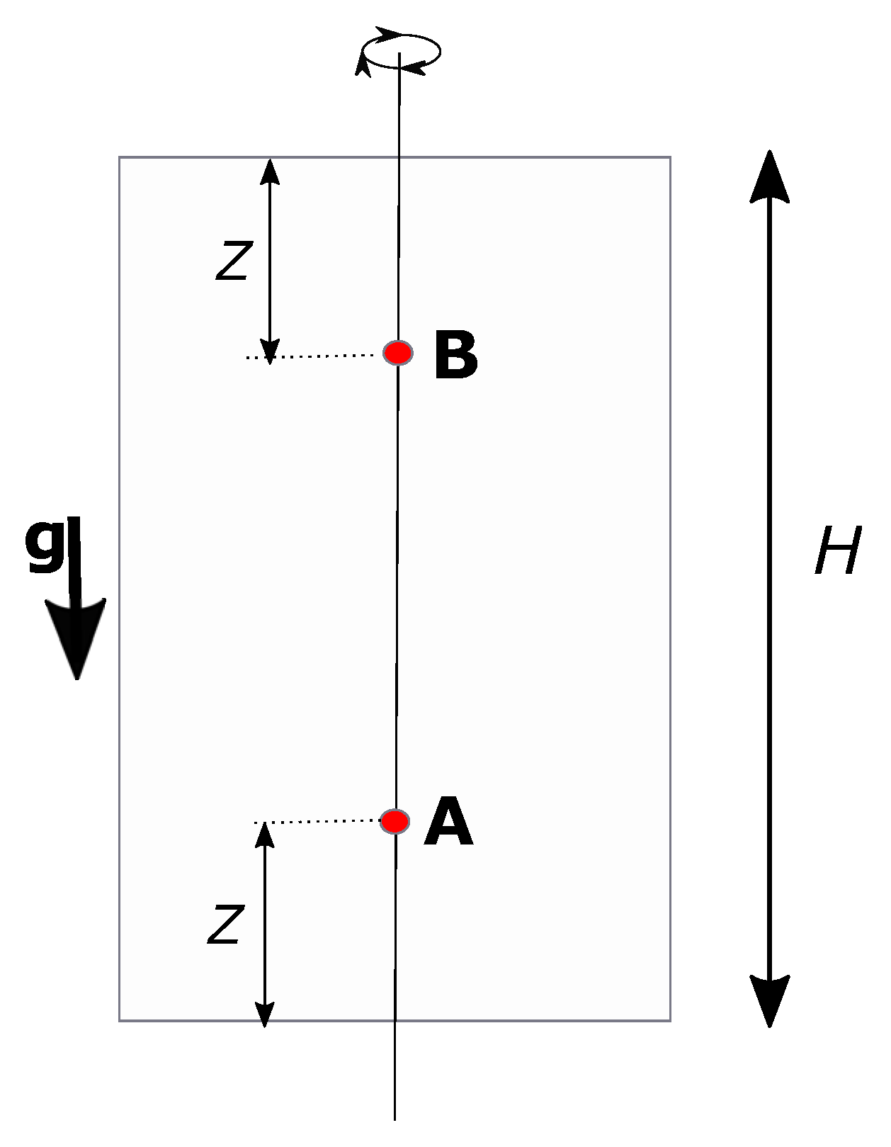
Pawlowski [1] describes laboratory experiments that are based on thermal convection for which the outcome clearly depends on parameter dependencies. The setup is very simple, as sketched in Figure 2. A closed cylinder containing the fluid at a constant low temperature T0 is put into a bath of elevated temperature T1. During the following phase in which the cylinder heats up, the temperature development within is recorded at two positions on the vertical cylinder axis. After the temperature in the entire cylinder has reached an ambient high temperature, the cylinder is put back into a bath with temperature T0. During the cooling phase that follows, the temperature at the two observation points is further recorded.
In the described experiments, the two temperature sensors are located on the cylinder axis at equal distances from the top and bottom of the cylinder. In Figure 2, the sensor positions are indicated by A and B. If heat conduction was the dominant process, both locations would show the same temperature graphs. In all of the experiments, however, convection comes into play, and the recorded temperature time series are quite different.
As convective motions strongly depend on the parameter dependencies on temperature, this has to be considered in the setup of laboratory experiments. The issue is outlined in detail by Pawlowski [1], describing the setup of an experimental series with the aim to find the optimal fluids for use in heat exchangers. While the cited study describes a theoretical approach, based on dimensional analysis, the aim here is to view the experiments from the modeler’s perspective. Using Computational Fluid Dynamics (CFD), i.e., numerical methods, we reconstruct the laboratory facility, choose the relevant formulations in terms of differential equations, and introduce the parameter dependencies. We examine the outcome of the constructed model and check the sensibility concerning numerical parameters and the temperature range. Finally, we compare the output of the numerical model with the results measured in the laboratory.
2. Differential Equations and Numerical Modeling
2.1. Differential Equations
Laminar flow, as can be expected for viscous fluids in the described setup, is described by the Navier–Stokes equations:
For the dependent variables pressure p and velocity v, ρ denotes density and μ the dynamic viscosity. Usually, the second term in the first Equation of (5) that accounts for inertia effects is neglected and the equation is reduced to Stokes flow [16]. The last term in the first equation is the forcing term that results from gravity. g is the vector with a length of 9.807 m/s2 in the direction of gravity, which is aligned here with the cylinder axis. Because of its relevance in the forcing buoyancy term, the variability of density is crucial for the onset of convective motions.
Heat transport is described by the advection–diffusion equation that can be written as:
where T is the dependent variable. C denotes the heat capacity and k is the thermal conductivity. Generally, all of the four previously mentioned parameters change as functions of temperature.
Altogether, the described equations denote a coupled system for flow and transport. Heat transport depends on the flow due to advective heat transport. The flow depends on the distribution of the transport variable due to the temperature dependencies of density and viscosity. Such coupled behavior is the origin of free thermal convection [17].
2.2. Numerical Model Setup
The breakthrough curves in the series of experiments outlined by Pawlowski [1] show a typical pattern (see below). Such regular behavior indicates that 2D convective motions are crucial, at least in the long run. 3D convection breaks the 2D symmetry of the setup and thus leads to complex irregular flow patterns. The modeling is thus mainly restricted to the exploration of 2D convective motions. Several runs with a 3D model are performed to check whether 3D eddies appear temporarily.
Due to the symmetry of the experimental setup, the 2D model region is half of a vertical cross-section through the cylinder that was shown in Figure 2, with the cylinder axis as a symmetry boundary. The region is a rectangle that, except for the symmetry axis, is bound on all sides by impermeable walls at a constant temperature (cylinder bottom, side, and top).
On the walls, we require a no-slip condition for flow, and a Dirichlet condition with a prescribed temperature. Along the cylinder axis, the symmetry conditions have to be fulfilled. Both the heating and cooling phases of the experiment are simulated by the model. For the heating phase, the initial temperature is low (T0) and the boundary temperature is high (T1). For the cooling phase, the initial temperature is high (T1) and the boundary temperature is low (T0).
Concerning the parameter dependencies, the first equation of the functional relations (4) is used. The focus here is on the experiments performed with SAE90 oil. So, we use the values given in Table 1 for the evaluation of the formulas for the different parameters.
Table 2 lists the reference parameters and geometrical values for the experiments. The values for density, dynamic viscosity, and diffusivity are for the reference temperature of 40 °C. The thermal diffusivity is computed using the definition D = k/ρC.
The model is set up using COMSOL Multiphysics 5.6 software that is very versatile for finite element numerical modeling of coupled processes in physics, chemistry, biology, geology, medicine, etc. In the 2D finite element formulation, the pressure field is approximated by linear variables (P1), velocity components, and temperature by second-order elements (P2). The mesh is irregular with a maximum element size of half a millimeter. A typical mesh consists of 5749 nodes, 10,344 triangular and 402 quadrilateral elements, and 22,996 degrees of freedom (DOF). The quadrilateral elements result from the special discretization of the boundary layers at the wall boundaries, as shown in Figure 3. For 3D linear elements for all dependent variables, a mesh with 23,835 nodes, 81,644 tetrahedra, and 16,320 prisms leads to 119,175 DOFs. With a value of around 0.9, the average mesh quality is very good in 2D, while the quality measure decreases to about 0.7 for the 3D mesh.
In order to stabilize the computation, we use consistent stabilization methods: Streamline and crosswind diffusion. Non-consistent stabilization is not used, in order to avoid unphysical numerical diffusion. The temporal development is simulated by time steps. The time steps are updated during the simulation according to the Courant–Friedrichs–Lewy (CFL) condition.
3. Results
A series of numerical runs were performed to explore the solution behavior, in order to compare it with the general observations of the laboratory experiments [1]. The effect of the temperature range was our particular focus. Numerical results with different T0 and T1 are reported below. The geometrical measures of the experiment were taken from the cited reference, where the SAE90 oil was used as the fluid. Concerning parameter dependencies, we mainly applied the values of Table 1. In some runs, we explored the effect of a changed a-value for the dynamic viscosity.
3.1. Flow Modeling
Figure 4 depicts flow patterns during the heating phase for the example simulation. The color plots show the velocity magnitude. Arrows indicate the flow direction. The run was performed for temperatures T0 = 22 °C, T1 = 95 °C, and the parameter dependency values of Table 1.
A strong convection current is initiated after the cool cylinder has been submerged in the hot water. There is strong downward flow in the center of the cylinder and upward flow at the outer wall. What follows is the weakening of the downward flow, while the upward flow component at the outer boundary resides. After around one and a half minutes in the lower center part of the cylinder, a strong upward flow appears, replacing the downward flow. In the subplots of Figure 4, the corresponding eddy can be recognized at t = 1.3 min, and it gains strength quickly, reaching a maximum height of a third of the column length at t = 1.9 min. After this dynamic phase, the recent eddy is pushed back by the major circulation. In the final phase, the system with a big circulation across the entire length of the cylinder and a smaller eddy at the bottom center retained between the eddies, the flow is downward, corresponding to upward flow along the outer wall and the lower symmetry axis. Small-scale instabilities appear at the bottom, as can be seen in Figure 4 at t = 2.5 min. These transients die out quickly.
The flow patterns of the cooling experiment are shown in Figure 5. As expected, many phenomena of the heating experiment appear during cooling as well, but in opposite directions. The dominating circulation has downward flow along the outer walls and upward flow in the center. Furthermore, after about 1.5 min, the formation of a second eddy can be observed, not at the center bottom of the cylinder but at the center top. While this eddy gains strength quite rapidly, it also shrinks quickly thereafter. In Figure 6, this circulation reaches its maximum at t = 1.7 min, and is reduced to its final much smaller size already at t = 1.9 min. The smaller disturbances, however, which in the cooling experiment appear at the top of the cylinder, look different compared to heating. Patterns, as shown at t = 1.9, show bigger eddies than in the first stage of the experiment. They appear and disappear in a quasi-oscillating temporal pattern, but never destroy the dominating two-eddy system.
3.2. Temperature Distributions
Figure 6 illustrates the temperature distributions at various stages of the heating and cooling experiments. The plots were taken from the output of the model run with the same parameters used for the plots in the previous figures. In the initial stage, one can see different heating patterns in the top and the bottom parts. These are attributed to the convection eddy that was observed in the flow pattern. The development of a second eddy corresponds to the appearance of a mushroom shaped plume, rising from the bottom along the cylinder axis, clearly to be seen at time t = 1.9 min. Later, with hotter fluid approaching the lower part of the cylinder from above, the strong thermal gradients in the upper part of the secondary eddy vanish. This corresponds to the final pattern, observed in the flow visualization, showing a weakened secondary current.
The temperature distributions during the cooling stage show similarities with the observations of the heating stage, but with exchanged roles concerning the top and bottom of the cylinder. In the initial phase, the fluid cools quicker at the bottom, while more rapid warming can be observed at the top when the cylinder is heated. Differences between the two stages of the experiment appear concerning the instabilities that follow the initial pattern. While there is a single rising plume during heating, more complex figures appear during cooling. The patterns, shown in Figure 6, are not stable. At certain time instances, a cool plume can be found halfway between the cylinder axis and wall (times t = 1.1 and 2.5 min), while there are also distributions with the three most significant plume in the center (t = 1.3). In the latter case, the relicts of previous plumes can be recognized. These figures reflect the complex flow patterns with multiple eddies, described in Section 3.1, that are more complex than during heating.
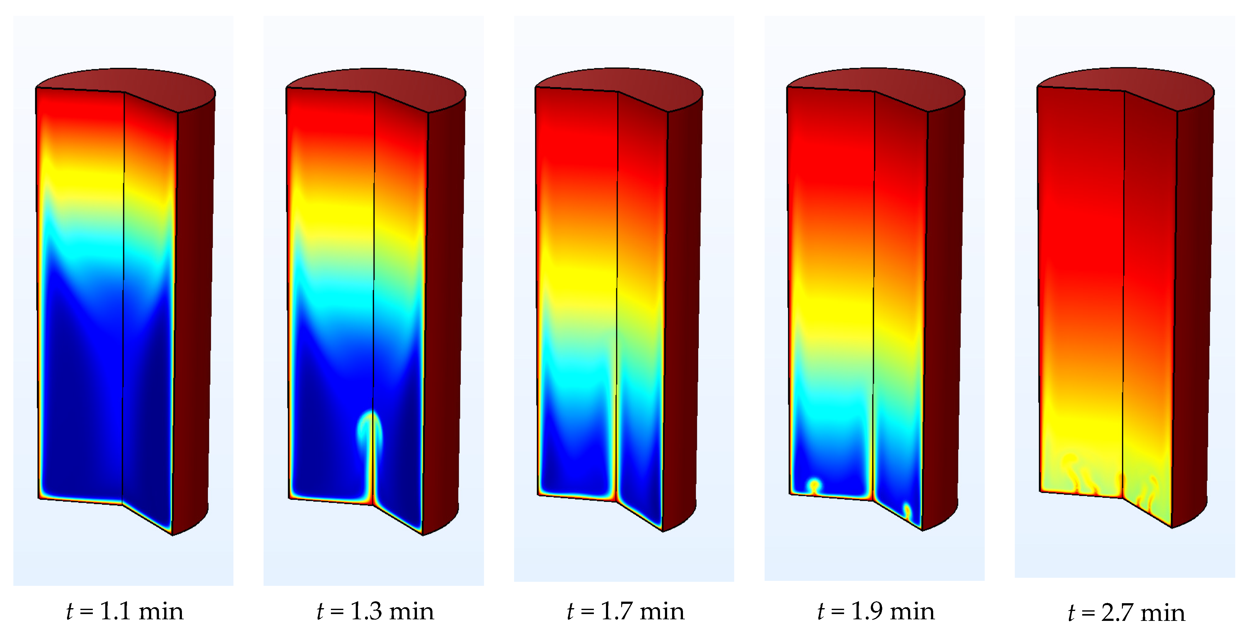
For higher temperatures T1, the patterns become more complex. As an example, Figure 7 depicts the temperature distributions during heating for changed T1 = 150 °C. The plume that rises along the cylinder axis appears earlier and reaches higher positions (t = 1.3 and 1.7 min). After reaching its maximum, the plume dissolves and a smaller off-center plume appears (t = 1.9 min). The behavior during heating resembles that described previously in the cooling stage. In the following, we even see patterns with several hot plumes rising from the bottom of the cylinder (t = 2.7 min). The system runs through a cycle of rising and vanishing secondary plumes several times. Each time, the plumes become smaller as the total temperature difference in the cylinder becomes smaller and the heating from the upper part of the cylinder reaches further downward.
4. Comparison with Laboratory Experiments
During the run of the experiments reported by Pawlowski [1], temperatures were recorded by two sensors. The locations of sensors A and B are indicated in Figure 1. In the described numerical runs, two ‘probes’ were included to simulate the sensor operation. Here we compare the obtained time-series, as far as it is possible.
The following figures show measured values (data, represented by markers) and numerical results (plotted curves) for the heating and cooling stages of the experiments. In the heating part, the markers and curves start at a low temperature value and end at a higher temperature, and vice versa in the cooling part, where the markers and curves start at a high temperature value and finally reach a lower temperature. Locations A and B are indicated in the legend.
In the report [1], measured data are depicted in a single figure. Similar to the above-described graphical representation, they are shown for heating and cooling, and for locations A and B. However, they are plotted as graphs. The markers in the figures here represent these graphs. The report [1] mentions the data as the typical output of the experiments, without providing a scale on the temperature axis. Using the numerical model, we explored various temperature ranges in order to check the match between these given data and the sensibility of the results for the temperature range. For the comparison in the graphs, the data curves were adjusted to fit the temperature range of the numerical model.
Figure 8 depicts a comparison between numerical and experimental results at both observation points, A and B, for the heating and cooling stages as described. The model was run with a low temperature of 22 °C and an elevated temperature of 33.4 °C. Obviously, there is no fit between model results and measured time series. The overall development is obviously correct, but its dynamics are much too slow, in two respects: (1) The transition from an initial phase with an almost constant temperature to a dynamic phase with strong gradients appears too late, with the exception of cooling in point A; (2) the gradients in the dynamic phase are smaller than the ones in the observed data. Moreover, the model cannot reproduce the peculiar behavior of the temperature curve at point B in the cooling experiment. There, a phase with small gradients was observed between phases with stronger gradients.
Numerous experiments with the numerical model were performed to obtain a better fit than the first attempt, shown in Figure 8, and to investigate the sensitivity to the temperature range. High and low temperatures were changed between 22 °C and 220 °C. In addition, we took into account that there must be a shift in time accounting for the conduction of the container itself to adjust to the changed ambient conditions. We also investigated initial disturbances in the dependent variables. Due to the replacement from one place to another, the cylinder may have been shaken and thus no longer contain the ideal initial values pressure and temperature distribution.
We observed that disturbances in the initial conditions do not have any effect on the results. The disturbances die out so quickly that they are hardly visible in the graphs. Moreover, we find that a shift of 30 s is convenient to obtain better fits with the laboratory data. From the temperature variations, it becomes clear that better fits are obtained for increased temperature ranges.
In all graphs, a partition into three phases can be observed: (1) There is an initial phase with almost constant temperatures; (2) a highly dynamical phase follows; and (3) finally, the temperatures monotonically approach the final state without any noticeable fluctuations. Figure 9 depicts the results for an increased value of T1 = 95 °C., in which the phases can be clearly distinguished. The legend indicates whether the graph is obtained from 2D or 3D modeling.
We first discuss the outcome of the simulations in 2D. At point A, the duration of the initial phase is predicted accurately for heating and cooling. At point B, the simulation shows a longer duration in the model than was observed in the laboratory. The dynamics that follow show monotonous graphs for point B in the heating experiment and point A in the cooling experiment. For point A during heating and point B during cooling, the development can be divided in two phases: The first with complex irregular behavior, followed by one with regular behavior. The irregular phase shows steep gradients (at A and B) as well as fluctuations (point B). These irregularities in the curves are surely an effect of local convective flow patterns.
For three of the four curves, the final development of temperature before reaching the new steady state is reproduced well by the results of the simulations. Only the development at point B in the cooling experiment does not match with the laboratory experiments. However, the curve seems to have shifted in time only. The length of the irregular behavior in phase 2 is much longer in the simulation than in the experiment, where a small ’swerve’ (German: Schlenker) was observed.
In addition to the results from a 2D model, Figure 9 depicts the output from 3D modeling. The rise of T observed during heating in the lab at position B is reproduced well, while the modeled rise at position A occurs too early. However, the curve does not show disturbances like the one from the 2D simulation. According to this, a phase with high dynamics does not appear.
The falling temperatures during cooling at location A coincide well with the real sensor measurements, while the comparison with the data from sensor B shows a large delay in the model. The curve itself is much smoother than that from the 2D model, indicating that there are not strong dynamics at intermediate times. There is a time period with steeper gradients, followed by smaller gradients—similar to what was observed in the laboratory. Nevertheless, in the model, this swerve appears after 4 and 5 min, while such behavior was observed in the real world in the initial stage for t < 1.5 min.
In order to demonstrate the effect of variable viscosity, a model run with constant viscosity was performed. Figure 10 shows the results for the same input values and parameter dependencies as those used for the illustrations of Figure 9. There are minor differences concerning the data for the cooling phase than for the heating phase. Figure 10 clearly demonstrates the symmetry of the model for constant viscosity. The results of heating and cooling stages can be mirrored on the horizontal axis in the middle of the relevant temperature range. Concerning the behavior of the entire system, the cases of heating and cooling are physically identical if the viscosity is constant.
The curves in Figure 10 were taken from a model run with constant viscosity, but with all other parameters dependent on temperature as illustrated in Figure 1. The complete symmetry of the model results depicted in the figure for the heating and cooling stages indicates that the parameter variability of the other parameters, thermal conductivity and heat capacity, is not relevant for the convective motions.
5. Discussion and Conclusions
The influence of parameter dependencies on thermal convection of viscous fluids was simulated by numerical modelling and compared with experimental results. Due to its strong temperature dependency, viscosity was of particular interest. The model output confirmed that the variability of other parameters (except density) is of marginal influence on convection.
The simulations show that the convection in the experimental facility can be divided in three phases: (1) An initial phase with a single eddy that has downward flow along the cylinder axis and upward flow on the walls, or vice versa, depending on heating or cooling; (2) followed by a highly dynamic phase with plumes emerging either at the bottom or the top, with the location depending on heating or cooling; and (3) a smooth development towards the final state with small secondary convective disturbances.
Concerning these phases, the models show minor sensitivity in phases (1) and (3), while the details of the convection patterns in phase (2) depend strongly on the chosen temperature range. While the development observed in the laboratory during phases (1) and (3) is captured well by the model runs, the deviations are highest in the dynamic phase.
The strong dynamics of phase (2) that are present in all 2D CFD simulations were not visible in the experimental results. In fact, during heating, the laboratory sensors recorded a continuous increase in temperatures at all times. For the cooling stage, only a small ’swerve’ (German: Schlenker) is mentioned in the report [1]. The time of this swerve roughly matches with the dynamic phase of the model output. A comparison of the eddies at the bottom of Figure 4 and at the top of Figure 5 for times t = 1.1 and t = 1.9 clearly shows the different patterns that lead to the differences in temperature development.
In the final phase, the biggest mismatch between numerical and experimental outputs can be seen during cooling at position B (see Figure 9). However, a time shift could make the curves match. The mismatch could thus be explained to be an effect of the mentioned difficulties to match the flow details in the preceding dynamic phase. If the model was to progress less dynamically in that phase, the transition to phase (3) would appear earlier. We can conclude that the computer model and laboratory experiment show different behaviors at times when the convective motion is strong.
The general behavior of the measured data, with a relatively smooth change at all times and a slight swerve of the temperature graph measured in the upper part of the facility during cooling, is better reproduced in the 3D simulations, although the timing does not match. As the dynamics in the 3D simulations are closer to the experimental data, we suppose that the strong dynamics seen in the 2D simulation are an artifact of the 2D approach, which in a real-world system is suppressed by the emergence of local 3D eddies.
Numerical modelling of viscous flows has advanced considerably for various situations. In comparison, the main characteristics of this study are (1) rotational geometry, (2) temperature dependency of viscosity, and (3) transient convection. Variations of the model setup, with and without the consideration of inertial effects, coarse and fine meshes, slender and widened boundary layer, modifications of parameter dependencies, etc., show that the results of the models presented here are very robust even concerning the dynamic phase. The stability of the numerical solutions can be seen as a verification of the model.
There are few studies in which numerical results are directly compared with experimental data. Here, a simple documented setup enabled modeling with only a few free parameters. Although the laboratory experiments are documented, some crucial information is not available. The cylinder material and the wall thickness are unknown, so a shift of the time scale due to the fact that the container has to adjust to changed ambient thermal conditions can only be guessed by inspecting the result. There is no comment concerning the variability of the experiment development on the temperature range. The way in which the sensors are fixed within the cylinder, and how the fixation may have influenced the hydraulic and thermal regimes, is not outlined.
For future research, it is recommended that experimental and modelling work should be performed in close cooperation. That enables the modeler to modify the CFD setting in a reasonable way. The experimentalist can modify the experiment, or include further sensors, to check on crucial points for comparison. The here-described experiment design is well suited for checking the effect of viscosity variations on convective motions.
Funding
This research received no external funding.
Institutional Review Board Statement
Not applicable.
Informed Consent Statement
Not applicable.
Conflicts of Interest
The authors declare no conflict of interest.
References
- Pawlowski, J. Veränderliche Stoffgrößen in der Ähnlichkeitstheorie; Salle + Sauerländer: Frankfurt am Main, Germany, 1991; ISBN 3-7941-3301-3. (In German) [Google Scholar]
- Sapunov, V.N.; Saveljev, E.A.; Voronov, M.S.; Valtiner, M.; Linert, W. The basic theorem of temperature-dependent processes. Thermo 2021, 1, 45–60. [Google Scholar] [CrossRef]
- Messaâdi, A.; Dhoubi, N.; Hamda, H.; Belgacem, F.B.M.; Abdelkader, N.; Ouerfelli, N.; Hamzaoui, A.H. A new equation relating the viscosity Arrhenius temperature and the activation energy for some Newtonian classical solvents. J. Chem. 2015, 2015, 163262. [Google Scholar] [CrossRef] [Green Version]
- Ike, E. The study of viscosity-temperature dependence and activation energy for palm oil and soybean oil. Glob. J. Pure Appl. Sci. 2019, 25, 209–217. [Google Scholar] [CrossRef] [Green Version]
- Cheng, C.Y. The effect of temperature-dependent viscosity on the natural convection heat transfer from a horizontal isothermal cylinder of elliptic cross section. Int. Commun. Heat Mass Transf. 2006, 33, 1021–1028. [Google Scholar] [CrossRef]
- Shivakumara, A.; Mamatha, A.L.; Ravisha, M. Effects of variable viscosity and density maximum on the onset of Darcy-Benard convection usinga thermal nonequilibrium model. J. Porous Media 2010, 13, 613–622. [Google Scholar] [CrossRef]
- Shivakumara, I.S.; Dhananjaya, M. Onset of convection in a nanofluid saturated porous layer with temperature dependent viscosity. Int. J. Eng. Res. Appl. 2014, 44, 80–85. [Google Scholar]
- Singh, K.; Sharma, P.K.; Singh, N.P. Free convection flow with variable viscosity through horizontal channel embedded in porous medium. Open Appl. Phys. J. 2009, 2, 11–19. [Google Scholar]
- Astanina, M.S.; Sheremet, M.A.; Umavathi, J.C. Unsteady natural convection with temperature-dependent viscosity in a square cavity filled with a porous medium. Transp. Porous Media 2015, 110, 113–126. [Google Scholar] [CrossRef]
- Holzbecher, E. The influence of variable viscosity on thermal convection in porous media. In Transactions on Engineering Sciences; Brebbia, C.A., Ed.; WIT Press: Southampton, UK, 1998; Volume 20, ISSN 1743-3533. [Google Scholar]
- Hossain, M.A.; Munir, M.S. Natural convection flow of a viscous fluid about a truncated cone with temperature dependent viscosity and thermal conductivity. Int. J. Numer. Methods Heat Fluid Flow 2001, 11, 494–510. [Google Scholar] [CrossRef]
- Hooman, K.; Gurgenci, H. Effects of temperature-dependent viscosity on forced convection inside a porous medium. Transp. Porous Media 2008, 75, 249–267. [Google Scholar] [CrossRef]
- Soares, A.A.; Ferreira, J.M.; Caramelo, L.; Anacleto, J.; Chhabra, R.P. Effect of temperature-dependent viscosity on forced convection heat transfer from a cylinder in crossflow of power-law fluids. Int. J. Heat Mass Transf. 2010, 53, 4728–4740. [Google Scholar] [CrossRef]
- Malkovsky, V.I.; Magri, F. Thermal convection of temperature-dependent viscous fluids within three-dimensional faulted geothermal systems: Estimation from linear and numerical analyses. Water Resour. Res. 2016, 52, 2855–2867. [Google Scholar] [CrossRef] [Green Version]
- Elder, J.W.; Simmons, C.T.; Diersch, H.-J.; Frolkovic, P.; Holzbecher, E.; Johannsen, K. The Elder problem. Fluids 2017, 2, 11. [Google Scholar] [CrossRef] [Green Version]
- Guyon, E.; Hulin, J.-P.; Petit, L. Physical Hydrodynamics; Oxford University Press: Oxford, UK, 2001; ISBN 978-0198517450. [Google Scholar]
- Bejan, A. Convection Heat Transfer; Wiley & Sons: New York, NY, USA, 2013; ISBN 978-0470900376. [Google Scholar]
Figure 1.
Parameter dependencies on temperature for SAE90 oil [1].
Figure 1.
Parameter dependencies on temperature for SAE90 oil [1].

Figure 2.
Vertical cross-section through the experimental setup, with cylinder axis in the middle.

Figure 3.
Part of the 2D model domain with mesh, showing triangular elements in the interior and quadrilateral elements on the boundary.
Figure 3.
Part of the 2D model domain with mesh, showing triangular elements in the interior and quadrilateral elements on the boundary.

Figure 4.
Flow patterns shown by velocity magnitude and arrows in the half cylinder cross-section for the heating experiment (maximum velocities in the subplots from left to right: 2.2, 2.4, 1.9, 3.9, 1.3, 1.0 mm/s).
Figure 4.
Flow patterns shown by velocity magnitude and arrows in the half cylinder cross-section for the heating experiment (maximum velocities in the subplots from left to right: 2.2, 2.4, 1.9, 3.9, 1.3, 1.0 mm/s).

Figure 5.
Flow patterns shown by velocity magnitude and arrows in the half cylinder cross-section for the cooling experiment (maximum velocities in the subplots from left to right: 3.1, 4.2, 3.7, 2.1, 1.3, 0.34 mm/s).
Figure 5.
Flow patterns shown by velocity magnitude and arrows in the half cylinder cross-section for the cooling experiment (maximum velocities in the subplots from left to right: 3.1, 4.2, 3.7, 2.1, 1.3, 0.34 mm/s).

Figure 6.
Temperature distributions in the cylinder; top: Heating stage, bottom: Cooling for T0 = 22 °C (blue) and T1 = 95 °C (red).
Figure 6.
Temperature distributions in the cylinder; top: Heating stage, bottom: Cooling for T0 = 22 °C (blue) and T1 = 95 °C (red).


Figure 7.
Temperature distributions at various times during the heating stage for T0 = 22 °C (blue) and T1 = 150 °C (red).
Figure 7.
Temperature distributions at various times during the heating stage for T0 = 22 °C (blue) and T1 = 150 °C (red).

Figure 8.
Comparison between measurements and numerical results, at two observation points, A and B, for the heating and cooling stages, for T0 = 22 °C and T1 = 33.4 °C.
Figure 8.
Comparison between measurements and numerical results, at two observation points, A and B, for the heating and cooling stages, for T0 = 22 °C and T1 = 33.4 °C.

Figure 9.
Comparison between measurements and numerical results, at two observation points, A and B, for the heating and cooling stages, for T0 = 22 °C and T1 = 95 °C with variable viscosity.
Figure 9.
Comparison between measurements and numerical results, at two observation points, A and B, for the heating and cooling stages, for T0 = 22 °C and T1 = 95 °C with variable viscosity.

Figure 10.
Comparison between measurements and numerical results, at two observation points, A and B, for the heating and cooling stages, for T0 = 22 °C and T1 = 95 °C, with constant viscosity.
Figure 10.
Comparison between measurements and numerical results, at two observation points, A and B, for the heating and cooling stages, for T0 = 22 °C and T1 = 95 °C, with constant viscosity.


Table 1.
Parameters and their dependency constants for SAE90 oil with Tref = 40 °C [1].
Table 1.
Parameters and their dependency constants for SAE90 oil with Tref = 40 °C [1].
| Parameter | Unit | Symbol | ζref | a | λ |
|---|---|---|---|---|---|
| Density | kg/m3 | ρ | 890 | −1200 | 1 |
| Dynamic viscosity | Pa s | μ | 0.202 | −17.9 | −0.201 |
| Specific heat capacity | J/(kg°K) | ρC | 2005 | 470 | 0 |
| Thermal conductivity | W/(m°K) | k | 0.11 | 4570 | 1 |
Table 2.
Parameters, units, and reference values.
| Parameter | Unit | Symbol | Value |
|---|---|---|---|
| Height | m | H | 0.075 |
| Diameter | m | d | 0.03 |
| Sensor location distance from top/bottom | m | Z | 0.012 |
| Dynamic viscosity | Pa s | μ | 0.202 |
| Density | kg/m3 | ρ | 890 |
| Diffusivity | m2/s | D | 6.78 × 10⁻⁸ |
| Low temperature | °C | T0 | 22 |
| High temperature | °C | T1 | 95 |
Publisher’s Note: MDPI stays neutral with regard to jurisdictional claims in published maps and institutional affiliations. |
© 2021 by the author. Licensee MDPI, Basel, Switzerland. This article is an open access article distributed under the terms and conditions of the Creative Commons Attribution (CC BY) license (https://creativecommons.org/licenses/by/4.0/).
Share and Cite
MDPI and ACS Style
Holzbecher, E. Parameter Variability in Viscous Convection. Fluids 2021, 6, 376. https://0-doi-org.brum.beds.ac.uk/10.3390/fluids6110376
AMA Style
Holzbecher E. Parameter Variability in Viscous Convection. Fluids. 2021; 6(11):376. https://0-doi-org.brum.beds.ac.uk/10.3390/fluids6110376
Chicago/Turabian StyleHolzbecher, Ekkehard. 2021. "Parameter Variability in Viscous Convection" Fluids 6, no. 11: 376. https://0-doi-org.brum.beds.ac.uk/10.3390/fluids6110376