
Diffusive Mass Transfer and Gaussian Pressure Transient Solutions for Porous Media

Center for Integrative Petroleum Research (CIPR), Department of Petroleum Engineering, College of Petroleum Engineering and Geosciences (CPG), King Fahd University of Petroleum & Minerals, Dhahran 31261, Saudi Arabia
Fluids 2021, 6(11), 379; https://0-doi-org.brum.beds.ac.uk/10.3390/fluids6110379
Submission received: 5 September 2021
/
Revised: 3 October 2021
/
Accepted: 11 October 2021
/
Published: 23 October 2021
(This article belongs to the Collection Challenges and Advances in Heat and Mass Transfer)
Abstract
:This study revisits the mathematical equations for diffusive mass transport in 1D, 2D and 3D space and highlights a widespread misconception about the meaning of the regular and cumulative probability of random-walk solutions for diffusive mass transport. Next, the regular probability solution for molecular diffusion is applied to pressure diffusion in porous media. The pressure drop (by fluid extraction) or increase (by fluid injection) due to the production system may start with a simple pressure step function. The pressure perturbation imposed by the step function (representing the engineering intervention) will instantaneously diffuse into the reservoir at a rate that is controlled by the hydraulic diffusivity. Traditionally, the advance of the pressure transient in porous media such as geological reservoirs is modeled by two distinct approaches: (1) scalar equations for well performance testing that do not attempt to solve for the spatial change or the position of the pressure transient without reference to a well rate; (2) advanced reservoir models based on numerical solution methods. The Gaussian pressure transient solution method presented in this study can compute the spatial pressure depletion in the reservoir at arbitrary times and is based on analytical expressions that give spatial resolution without gridding-meaning solutions that have infinite resolution. The Gaussian solution is efficient for quantifying the advance of the pressure transient and associated pressure depletion around single wells, multiple wells and hydraulic fractures. This work lays the basis for the development of advanced reservoir simulations based on the superposition of analytical pressure transient solutions.
1. Introduction
This article shows how the advection and diffusion terms in the equation for convective mass transport by Fokker–Planck can be solved for use in certain types of pressure-driven flows, typically caused by engineering intervention in geological reservoirs. The result is an expression with exponential terms for the probability position of particles transported by the convective process, both for advection driven by migrating pressure gradients and for the random walk diffusion.
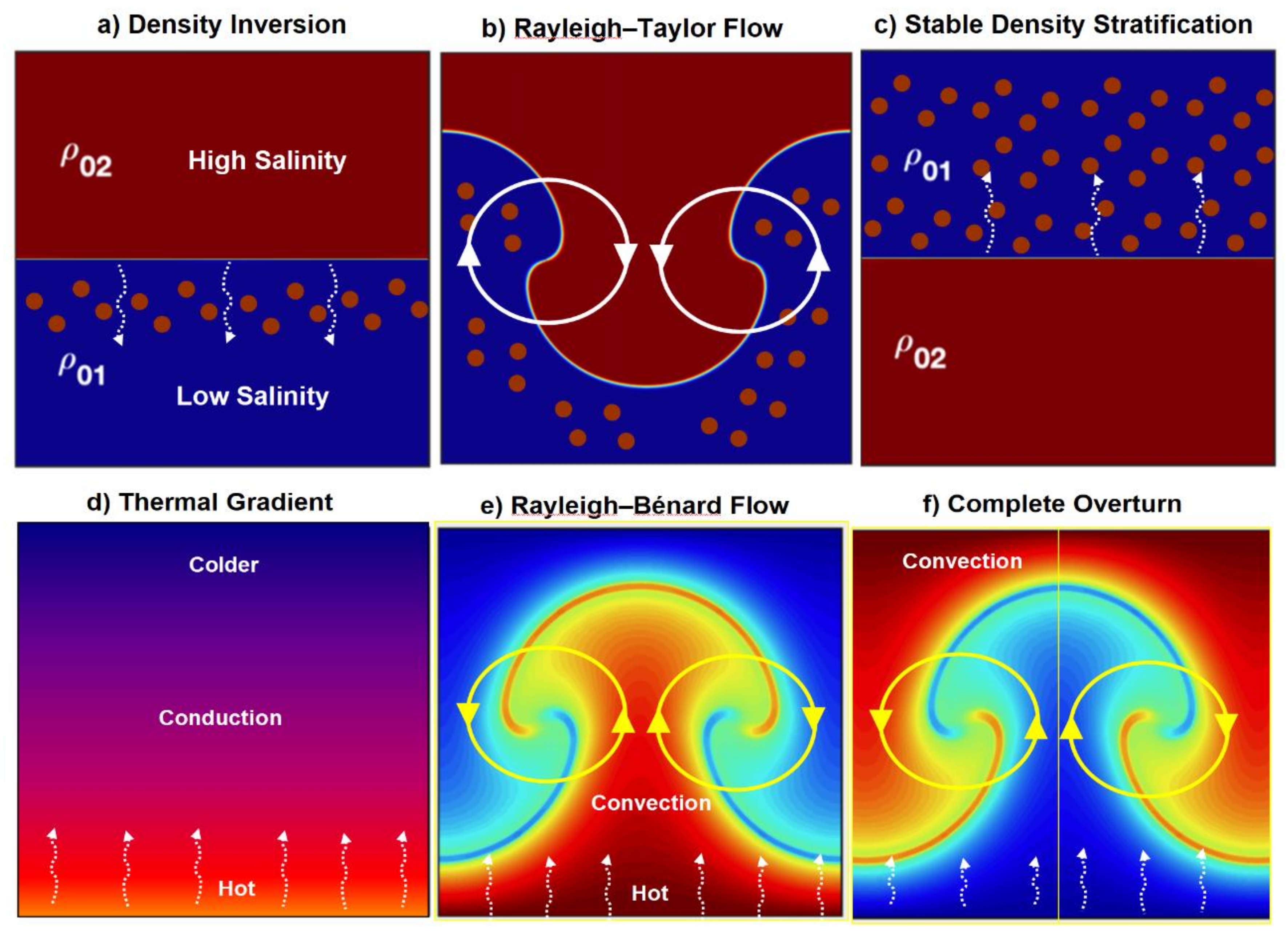
Before setting out to derive the computational solutions, it may be useful to describe some typical examples of situations where advection and diffusive mass transport may occur jointly, as summarized in the principle sketches of Figure 1. The examples of mass transport systems are ranked from relatively simple (mass transport only) to more complex cases (mass and heat transport) based on the number of scaling parameters involved.
First, consider a high salinity layer resting on top of a low salinity layer (due to heavy evaporation at the surface of the upper region in a brine-filled basin). The early density inversion between the two liquid regions triggers a fast advective flow, due to Rayleigh-Taylor (RT) instability, and is accompanied by relatively slow diffusion (Figure 1a–c). After the removal of the earlier inversion of the density layering by advection, the further diffusion of the high salinity solute toward the lower density layer will remove the density gradient asymptotically altogether and will be completed at an infinite time.
Next, consider a Rayleigh–Bénard (RB) flow due to thermal convection (Figure 1d–f). The process accelerates the transfer of heat from the hotter bottom plate to the colder surface by the convective mass transport of fluid initially at the bottom boundary. This process drives the mixing of the liquid outer core of our planet that maintains the magnetic field, as well as the crystalline creep of olivine-rich rocks in the upper and lower mantle that drives the movement of tectonic plates at the Earth’s surface [2].
One way to describe the mass transport dynamics of the above processes is by starting out with a Navier–Stokes equation that can be parameterized to split the key physical forces, such as those due to the external pull of gravity, the advective flow and acceleration thereof and divergence due to diffusion and internal flow sources [3]. Ruling out inertia, the studied flows can be assumed to be only governed by advection and diffusion; non-dimensional scaling parameters can be introduced to weigh the relative importance of the two principal components of the mass transport process.
For example, the Péclet number (Pe), which is the ratio of advective and diffusive transport rates [4,5] is adequate to describe the RT instability:
with molecular diffusivity , advective flow rate , and the length unit . For Pe << 1, the diffusive transport rate dominates the mass transport process; for Pe >> 1, the advection is more important than diffusion. Clearly, for the saline solute of Figure 1a–c, Pe >> 1 applies for the early phase (Figure 1a), when the density inversion is removed by the RT flow (Figure 1b), and once the density stratification is no longer inverse (Figure 1c), the advective transport ceases altogether, such that Pe = 0 from there onward. The principles of dynamic scaling of the Navier–Stokes need to be observed when building RT models and can be expanded to non-Newtonian fluids as long as the requirement of rheological similarity is observed [6].
For the RB flow in Figure 1d–f, the relative rates of heat transport by advective mass transfer and by conduction (heat diffusion) are given as a ratio in the Prandtl number [3,4]:
with the kinematic viscosity, , of the convecting fluid and thermal diffusivity, . For Pr << 1, the diffusive transport rate dominates the mass transport process; for Pr >> 1, the heat transport by advection is more important than thermal diffusion. Experimental studies of thermal convection in high Prandtl number silicones provide excellent analogues for studying mixing and deformation patterns involved in mantle convection [7,8,9].
A third example (examined in more detail in the main analysis) considers a subsurface reservoir with advective flow maintained by a pressure gradient with possible net displacement contributions by diffusion (Figure 2a). Water is injected into an oil reservoir via hydraulic pressure on inlet valves (in the left-side of reservoir space) to sweep non-residual oil via the interconnected pore spaces in the permeable rock to the array of producer wells (on the right-side of reservoir space) to extract the hydrocarbon. Similar well patterns are used to extract geothermal energy, producing hotter reservoir fluids after injecting colder fluids, leaving a positive energy balance for use in human engineered appliances, vehicles, factories, offices and housing. Such flow systems are governed by the same Péclet number as for Figure 1a, and when the pump rate is steady, the flow rates in the reservoir will only change slowly due to overall pressure depletion in the reservoir, such that Pe will remain in a narrow range over the entire production process. The detailed map view of Figure 2b highlights how tracers inserted at time zero as an instantaneous mass will form diffusive plumes traveling downstream, assuming Pe ≈ 1. These diffusive plumes are not to be confused with advective plumes due to Rankine flow with continuous source injection, where the shape of the plumes is controlled by the Rankine number (Rk, first defined in Weijermars et al. [11]). In the case of Figure 2b, the tracer mass is injected in an early instant, and the plumes are controlled by the relative rate of the diffusive and advective flow—henceforth, the Péclet number (Pe).
The remainder of this article proceeds to succinctly review the description of diffusive mass transfer by probability density functions for the dilution of tracer concentrations. It is first shown how to solve for the probabilities of the diffusion term in the Fokker–Planck equation for convective mass transport (Section 2). The result is then transposed to also accurately describe the advance of pressure transients that drive the advective fluid transport due to a pressure gradient introduced at time zero (Section 3). The initial approach is kept as simple as possible by assuming 1D or 2D flow in an infinite lateral reservoir (such as applies to unbound flow regions around hydrocarbon wells in shale oil and gas plays).
2. Diffusive Mass Transports
The mathematical theory of diffusion in fluids is founded on the transformation of heat conduction equations [12,13,14]. The spatial transport of molecules from one part of a system to another by random motions is termed a diffusion process [15,16]. The paradox of diffusion is that whilst it is impossible to say in what direction the individual molecules will move in their random walk, it is possible to calculate the mean distance traveled over a certain period, starting from a position where there is an initial higher concentration of molecules. Although no single molecule can be assigned a particular direction of motion, the random molecular motions and collisions result in a spatial net transfer of tracer molecules from the higher to lower concentration regions as long as there are more molecules in the higher concentration portion of the fluid.
2.1. Diffusion in Various Dimensions
In fluid systems with isotropic diffusivity, the rate of a unidirectional (1D) diffusion (e.g., due to planar source in the origin normal to the x-axis) through a unit area of observation planes (Figure 3a), also oriented normal to the x-axis, away from the source) is proportional to the concentration gradient measured normal to the section (e.g., Crank [16]):
where [MT−1] is the rate of diffusive mass transfer per unit area of section, [ML−1] is the mass concentration in a certain location of the diffusing substance, expressed as a mass per length (in the average diffusion direction), [L2T−1] is the diffusion coefficient (also termed diffusivity), and x [L] the space coordinate using a reference frame with the (y,z)-plane hosting the initial mass deposited there instantaneously at time zero. If we are mostly interested in the spatial change of the concentration over time, a simple expression results [16]:
This expression is analogous to the diffusion part of the Fokker–Planck equation (e.g., Risken [17]), which describes the change of diffusive particle density from an initial disturbance as a probability of future spatial values consequent to advection and diffusion :
We first focus on the diffusion process and assume a case where advection is absent, simplifying Equation (5) to
When the diffusion is only studied in one dimension (in a direction appropriately oriented with respect to the planar source), Equation (4) may be simplified into
The general solution of Equation (7) for a fluid concentration [ML−1] originating from a finite quantity of mass [M] placed in the planar source diffusing into an infinite 1D lateral direction is [18]
Similarly, the diffusion equation for a mass [M] concentrated in a cylindrical source aligned with the z-axis at the origin of a 3D reference frame (Figure 3b) is
The general solution of Equation (9) for the fluid concentration [ML−2] diffusing into an infinite 2D lateral planar space is [16]
Ultimately, the diffusion equation for a singularity mass in the origin (Figure 3c) through a 3D space with isotropic diffusivity is
The general solution of Equation (11) for the fluid concentration [ML−3] due to a finite mass quantity diffusing into an infinite 3D space is [16]
Equation (12) uses a scalar for diffusivity and therefore assumes the diffusion occurs in isotropic media. The adaptation of Equation (12) to account for anisotropic diffusion is straightforward and requires the introduction of a diffusivity tensor (see Section 3).
2.2. Scaling the Initial Mass Concentration
The initial mass concentration in location x = 0 after one time unit (remember the diffusivity has dimensions [L2T−1]), for the 1D diffusion case will be scaled (from Equation (8) equating to ) by = [ML−1]; for the 2D diffusion case we, have (from Equation (8)) = [ML−2]; for the 3D diffusion case, we have (from Equation (10)) = [ML−3].
To observe the dilution process for the three basic cases of Figure 3a–c, one should monitor the decay of the concentrations in the dashed observation planes (1D, 2D) and regions (3D) and use the initial dimensional units of for each case, which are [ML−1], [ML−2], and [ML−3]. For the same initial concentrations (rebased to mutual units) and the same diffusivity, the dilution via dispersion of molecular particles will be fastest for the spherical source geometry, intermediate for the cylindrical source and slowest for the planar source.
Reverting to the representation of the transient diffusion front profile as a normalized probability distribution, , as in the Fokker–Planck formulation of Equations (5) and (6), the Gaussian equations for the 1D, 2D and 3D diffusion cases are solved by taking the respective ratios of and :
scaling as the inverse of the variance (squared standard deviation at each time step), such that is a time-dependent scaling factor (also termed the precision). Evidently, accounts for the decay of the initial concentration after each time step, because
The solution of Equation (14) is universal, with the understanding that for application to 1D diffusion problems, two dimensions are annulled (e.g., y = 0 and z = 0), and for 2D diffusion problems, only one dimension vanishes (e.g., z = 0). For the respective 1D, 2D, and 3D diffusion cases, has dimensions [ML−1], [ML−2], and [ML−3], which can be succinctly written as
with n = 1, 2, 3 for 1D, 2D and 3D diffusion cases. Consequently, the Gaussian probability solution of Equation (14) is universally valid for 1D, 2D and 3D diffusion cases, when using as defined in Equation (15). The latter equation basically shows how the quantity M needs to be replenished at each time instant in balance with the dilution rate at the source, such that keeps the same amount of M to diffuse.
2.3. Using Regular Probability versus Ascending and Descending Cumulatives
A persistent misconception prevails in the literature about the computation of the probability of the concentration values, , occurring at various travel distances in the resultant direction of random-walk diffusion. According to the present study, the probability of these concentrations for 1D, 2D and 3D cases are directly given by Equation (14). However, a majority of users continue to use not the regular probability but the descending cumulative (based on integration of the area under the regular probability curve; e.g., Crank [16]). The mitigation of this widespread misconception warrants a brief explanation, with examples, of how to properly interpret the various probability density functions for the solute concentrations due to diffusion from an instantaneous initial source mass.
First, consider the dimensional probability density function, (Figure 4) for the 1D case of Equation (8), which can be written in terms of the standard deviation, :
The ascending cumulative distribution function, , describes the likelihood that a fraction of the original amount of tracer (or solute) has not yet reached the location x, expressed as using the error-function (erf):
Note that Equation (17) has the form of a two-sided Laplace transform, which was applied by Fourier [12] to develop the heat diffusion equations subsequently used by Fick [13] to develop the diffusive mass transport equations.
If we limit our attention to the cumulative distribution in the half-space with positive x-coordinates, the factor ½ can be dropped (rescaling the vertical axis from 0.5 to 1 at x = 0) from Equation (17):
Figure 5a shows examples of the ascending cumulative for different times (100 years, 10,000 years, 1 million years and 10 million years). These integral solutions show the volume under the curve (fraction of the original amount of tracer) that has not yet reached a certain location at a particular time. For example, after 1 million years at 40 m from the source, a 40% fraction of the initial mass has still not reached the location (but 60% has). At x = 100 m, 80% of the initial mass has still not reached the location (but 20% has).
Another way to plot the cumulative is the descending cumulative distribution function (also called survival function) , which is obtained from the ascending cumulative of Equation (17) by applying :
The operation means that now the complementary probability is given, namely . The reference is now the probability of which fraction of the original mass was already brought by diffusion past location x. If we again limit our attention to the cumulative distribution in the half-space with positive x-coordinates, the factor ½ can be dropped from Equation (19):
Using the error-function complement (erfc) defined above, Figure 5b shows examples of the descending cumulative or decumulative probability function for different times (100 years, 10,000 years, 1 million years and 10 million years). These integral solutions show the volume under the curve (fraction of the original amount of tracers) that have already reached a certain location at a particular time. For example, after 1 million years, at 40 m from the source, a 60% fraction of the initial mass has already reached the location (but 40% has not). At x = 100 m, 20% of the fraction has already reached the location (but 80% has not).
3. Advective Mass Transports Due to Pressure Gradients
The early mathematical description of heat diffusion by Fourier [12] led Fick [13] to apply the equations to mass diffusion. The application to pressure transients was furthered by Raghavan [20] in the context of well test analysis. Traditionally, the advance of the pressure transient is modeled analytically by scalar equations (developed by petroleum engineers in well testing literature) that generally do not attempt to solve for the spatial vector field solution for the position of the pressure transient as it migrates over time. The classical well testing equations are used to estimate the change over time of the average pressure in the reservoir in order to be able to estimate certain unknown properties (such as permeability) of the reservoir rock from which the fluid is produced [21,22,23].
3.1. Current Practice in Reservoir Modeling
Prior attempts have been made to develop a so-called Fast Marching Method (FMM) to go beyond the limitation of classical well testing formulae and reconstruct the spatial advance of the pressure front [24,25,26,27]. Such methods are particularly needed to develop reservoir simulators that can quickly resolve for the flow near hydraulically fractured wells, presently used to develop geothermal and hydrocarbon reservoirs around the globe. FMM results for the advancing fluid due to a pressure gradient have been compared to results using analytical vector field solutions based on complex analysis methods (CAM), augmented with Eulerian time-tracking, and both methods were found to be accurate [27]. However, FMM models can presently only account for simple fracture geometries, and the spatial solution of the pressure front requires gridding to compute the shape of the advancing pressure transient cell-by-cell at different times.
3.2. Gaussian Pressure Transient Solution
For the reservoir studied here, we assume the pressure in the reservoir remains above the bubble point pressure of the reservoir fluid to avoid multiphase flow conditions complicating production in condensate and wet gas reservoirs. The fluid is of constant density and constant Newtonian viscosity, has constant compressibility throughout the reservoir and is not sensitive to pressure changes introduced by engineering interventions. The process is isothermal. The porous medium hosting the reservoir fluid is also considered homogenous and isotropic in porosity and permeability. The solutions are confined to convective flows with mass transport in the laminar flow regime, without the inertia effects which are typically absent in flow in porous media.
The purpose of the present study is to demonstrate the concept of the Gaussian pressure transients as a method to model the advance of the pressure transient and the associated pressure depletion in the prototype reservoir. The Gaussian method is completely new and is first launched in this paper, so there is no prior work to which to refer (except a parallel conference paper [28], which applies the concept in a practical study). Spatial changes in the porosity and permeability are not considered in the present study but can be accounted for by the spatially zoned indexing of the diffusivity. Zones with lower diffusivity will locally decrease the pressure gradient; zones with higher diffusivity will locally increase the pressure gradient. Fractured porous media can be perfectly modeled with the Gaussian method because the fractures have finite widths and lengths, where the diffusivity will be much higher than in the nearby matrix; the results will be a locally higher-pressure gradient. Detailed solutions for heterogeneous, anisotropic and fractured reservoirs will be given in future work, based on the present foundation.
A key step made here is that we show how the diffusion equation can be adapted for the rapid generation of transient pressure profiles, due to certain engineering interventions in porous media that begin with the introduction of instantaneous pressure drops. The bottomhole pressure is quickly lowered by the presence of the well, and the initial flow is then commonly held constant with the help of a pump, for which a variety of technical solutions exist. Rather than weakening or diluting at the source, the pressure will stay constant, while almost instantaneously diffusing into the reservoir. The advance of the pressure transient is not linearly related to the fluid withdrawal rate [29,30].
The equation for pressure diffusion into the 1D space of a porous medium is
which is identical to Equation (7) for molecular diffusion except for the use of hydraulic diffusivity in Equation (20) and molecular diffusivity in Equation (7). In reservoir studies, we are commonly dealing with a pre-existing pressure in the reservoir, , which is then suddenly changed by an engineering intervention (e.g., producer well and hydraulic fractures). Thus, a local pressure change is also commonly imposed, , which is the difference between the original pressure in the reservoir, , and the pressure level of the well intervention , such that the initial pressure in Equation (21) can best be replaced by , in order to avoid any confusion:
The Gaussian general diffusion solution of Equation (14) can now be used for tracking the spatial and temporal change of the pressure in a 1D, 2D or 3D reservoir layer as the pressure front advances from the source into the reservoir. The spatial advance of the initial pressure change, , can be accurately described by the general solution for the 3D Gaussian diffusion probability equation:
Equation (23) is extremely useful to model the spatial pressure-depletion profile around individual wells and hydraulic fractures.
Recall that for the isotropic diffusivity case. For application to layered reservoirs in the geological subsurface, it is practical to introduce the diffusivity tensor, (dropping the subcript h). If we next chose the reference frame aligned with , then the diffusivity tensor elements all vanish, except the principal ones such that (n = 1, 2, 3) can be equated to , and . The solution of Equation (14) can now be modified to account for anisotropic diffusivity:
Reservoir development target zones (aquifers, geothermal and hydrocarbon reservoirs) occur commonly confined between an upper and lower impervious boundary, with the overlying and underlying formations being bound by relatively clay horizons or other impermeable strata. Consequently, we may conveniently reduce our analysis to a 2D pressure diffusion problem.
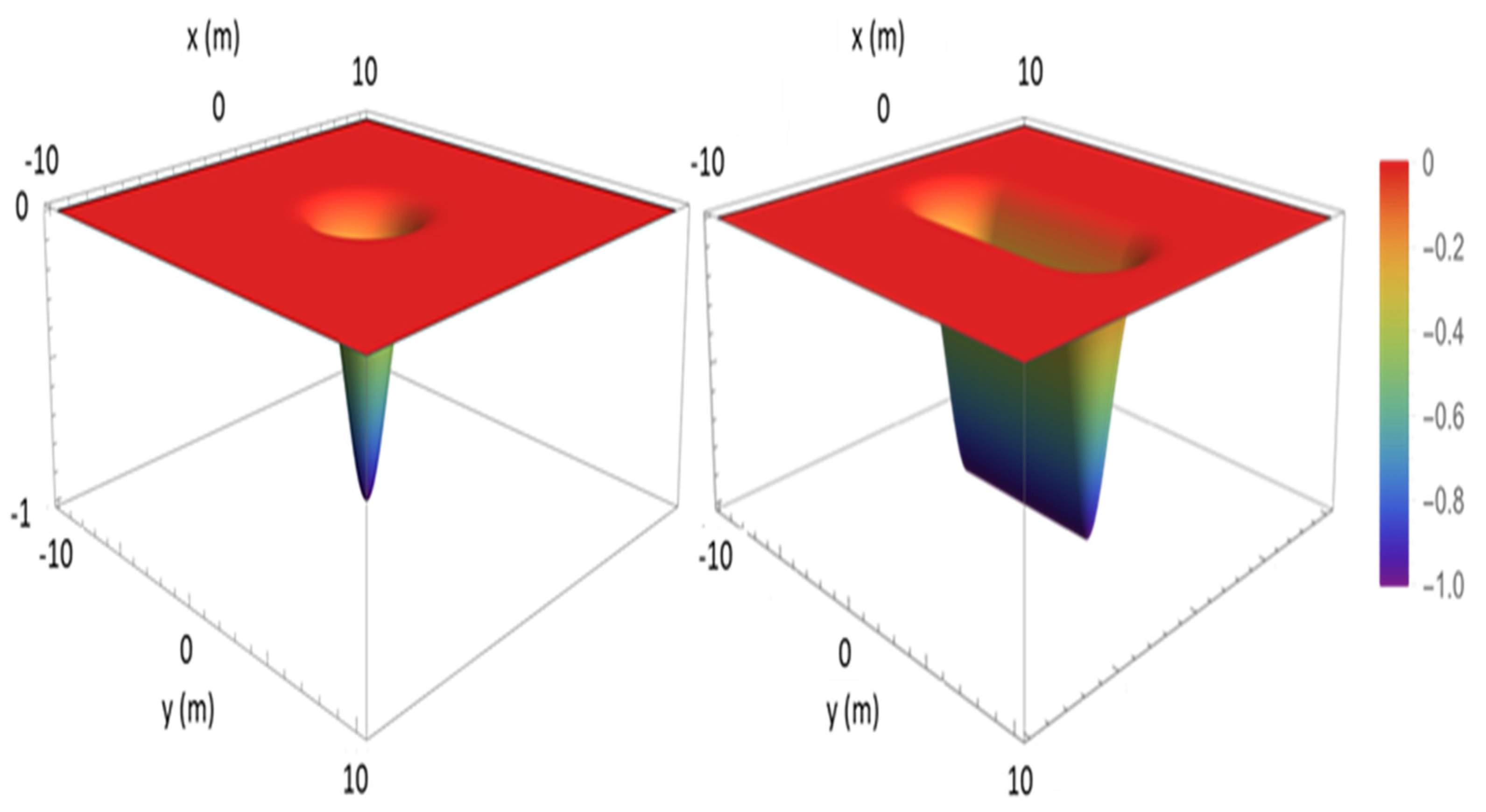
If the well system is a simple vertical well in pressure communication with the full height of the reservoir zone (via a bottom-hole gravel-pack with well perforation), it would act as a 2D cylindrical source of pressure change (Figure 3b). The pressure transient will advance in the reservoir as concentric circles of radius () in a 2D map view and as a cone in a 3D perspective (Figure 6a).
For the pressure changes induced by a single hydraulic fracture of half-length , we have elliptical pressure-change contours (Figure 6b). A conditional modification is introduced to ensure that the transient propagates at the same rate in all directions away from the initial pressure drop source, as follows (assuming the fracture runs parallel to the y-direction):
- For , use ;
- For , use ;
- For , use .
The evolution of the 3D pressure profiles around multiple sources of pressure change in the reservoir space (for example, n wells or n hydraulic fractures) can now be determined using a series of (time-dependent) Gaussian equations to represent the reservoir pressure at any one time:
Multiple pressure profiles may interact (as in Figure 7) by shifting the center of pressure change coordinates (x, y) in Equation (26) to a new location (x’, y’), applying a simple coordinate translation transformation to Equation (26):
For fractures that are obliquely oriented, at angle with respect to the Cartesian x-direction, we may introduce an additional coordinate rotation transformation:
However, in the present study, we keep the fractures aligned with one of the Cartesian axes for simplicity.
3.3. Engineering-Induced Pressure Depletion in Reservoirs
To pair the profile of the pressure transient of Equation (25) to reservoir parameters, we introduce the time-dependent spatial advance, , of the pressure transient (radius of investigation, see Appendix A in [30]):
With the hydraulic diffusivity, , capturing the intrinsic properties of the reservoir (, ) and of the fluid (, ) in its pores:
with porosity, , permeability , dynamic viscosity, , and total compressibility, . If the time scale, , is in hours and all parameters are inserted as imperial field units, the conversion constant, Z, for physical units used in Equation (29) will assume the value of 1688.7 [30]. Note that the time is sometimes formulated in terms of a diffusive pseudo-time , with the square root of time unit () (e.g., [24,25]), such that effectively
The advancing pressure transient can now be tracked by equating the precision to . Examples of the pressure transient profiles for 4 fractures with half lengths of 10 m and a fracture spacing of 10 m were plotted for 4 successive production times (Figure 7), using the reservoir properties given in Table 1.
One important limitation of well testing literature is that attempts have been made to include, in the conversion factor Z, additional corrections to account for initial conditions in the reservoir other than a single well acting as a cylindrical source for the pressure diffusion. For example, modifications of Z have been suggested for wells with bi-wing fractures, for wells in finite cylindrical reservoir space and drainage regions with rectangular shapes [20]. All these approximations may be assumed to be of limited accuracy. The Gaussian superposition method introduced here does not suffer from such inaccuracies, because if metric units are used, Z = 1/2 for all cases. The explanation is that the interference of the pressure transients for multiple sources is accounted for in the models, including the formation of bounded flow cells when multiple wells are placed in close proximity.
It appears now to be possible to model (in future work) increasingly complex flows by the superposition of pressure sources and then next solve for the pressure gradient field, streamlines, velocity field, time-of-flight contours and any other parameters relevant for evaluating reservoir and well performance. Having solved the pressure field, the aforementioned derivatives follow standard equations and involve no computational complexity that would prevent the implementation of the proposed method in a full-scale reservoir model.
4. Discussion
Well testing literature has occasionally attributed the advective movement due to a pressure gradient to a diffusion process [20,31]. The present study argues that the advance of pressure transients, the gradient of which drives transport that has been traditionally labeled as advection, can be described by Gaussian solutions, similar to Fourier descriptions of molecular random walk diffusion with net mass transport. In fact, both processes—i.e., the random walk diffusion and the pressure transient advance—can be described by Fourier solutions, with the respective diffusivity terms being the key control parameters for the relative rate of advance. This insight is practical to simplify descriptions of mass transfer dynamics in geological reservoirs.
Additionally, the three fundamental types of sources (planar, cylindrical and spherical; see Figure 3a–c) can adequately describe even very complex flow cases by superposition. Our principal focus is on diffusion phenomena in geological reservoirs with laterally large dimensions, which justify the assumption of an unbound porous medium. When diffusion occurs in finite spaces, correction factors can be introduced, as has been exhaustively documented elsewhere [32].
Interestingly, acoustic pressure waves in the subsurface are routinely described by Green’s functions to solve integrals that are related to Fourier transforms similar to those at the basis of diffusion equations. However, the equations used to describe the propagation of elastic pressure waves generated from a source such as seismic guns and vibroseis trucks are not (directly) suitable to solve pressure diffusion in the fluid phase of porous reservoirs.
4.1. Comparison of Gaussian Pressure Transients
The pressure profiles generated here with the Gaussian method appear similar to those generated in our research group with advanced reservoir simulation methods; see for example Figure 4 in Nandlal et al. [27] and Figure 1 in Weijermars et al. [33]. After about 1.4 months (1000 h) of production, the pressure depletion fronts initiated from the BHP of the individual hydraulic fractures meet and coalesce (Figure 7, second image from left). After about 6.8 months (5000 h) of production, the pressure in the central matrix zones between the fractures has largely become pressure-depleted (Figure 7, third image from left).
After pressure depletion in the matrix zones between the hydraulic fractures, the pressure transient advances (by diffusive transport) outward from the central fracture box (Figure 7, fourth image from left), as explained with detailed flow regime correlations from well data in our prior studies [33,34]. The reservoir fluid is then drained laterally from the reservoir via the fracture tips. However, the fluid withdrawal from the reservoir by convective transport-in ultra-low permeability rocks lags behind the pressure transient advance [29]. The lag between the diffusive and convective time-of-flight is the reason for the low recovery rates of shale wells, even when hydraulically fractured (work cited). The pressure depletion in the central fracture box (Figure 7, fourth image from left) may not be equated with full fluid withdrawal, as was modeled in detail in another prior study by our group (see Figure 18 in Parsegov et al. [35]).
The present study considers the pressure transient rate based on diffusivity solutions that abide with Darcy flow (as the hydraulic diffusivity inputs are based on Darcy’s Law). In fluids such as gases where non-Darcy flow contributions become increasingly relevant when the porous medium has nanoDarcy permeability, the diffusivity term should be adjusted accordingly to account for molecular diffusion effects. Some thoughts in this direction have been expressed by other authors ([36] and references therein). Other diffusive effects such as thermo-diffusion and Soret effects [37] may need to be factored in as well.
4.2. Merging Gaussian and Complex Analysis Methods (CAM)
Another fast analytical solution method for fluid flow in reservoirs based on Complex Analysis Methods (CAM) was previously advanced by our research group [34]. CAM models are gridless and based on analytical solutions with infinite resolution [27,38]. As both CAM and Gaussian models are gridless and continuous, the outcomes of these models can be merged and spatially superposed, sidestepping any tedious coupling of codes as needed in finite difference-based methods.
Some conceptual differences between the CAM and Gaussian methods can be utilized to obtain a more versatile toolbox for the ungridded modeling of fluid flow in fractured porous media. For example, CAM starts out as a solution of the bi-harmonic equation for steady flows, which gives the instantaneous velocity field for the flow. Transient flows can also be modeled with CAM by superposing, with short time-steps, the solutions of the bi-harmonic equation when fluid sources wax and wane or follow a time-dependent function. However, the pressure field is solved instantaneously for each steady case snapshot in time, due to which the modeling of pressure transients with CAM is not possible. Another inconvenience of CAM solutions is that it is possible to arbitrarily assign strengths to the flow attributes (such as high permeability fractures), but these strengths may, in fact, be higher than physically feasible in porous media; an upper limit therefore needs to be observed in order to avoid the occurrence of models with arrays where the velocities overshoot the adjacent fractures.
In contrast to CAM-based flow descriptions, the Gaussian method proposed here initially solves the pressure field at any moment in time as a starting point. From the pressure gradient field, we may subsequently compute the spatial velocity field. An advantage of the Gaussian methods is that the superposition of pressure depletion profiles from various sources cannot result in flow overshoot, because the boundary condition is imposed by a certain bottomhole pressure of the well system and the initial reservoir pressure.
5. Conclusions
This paper expresses the random walk probability of diffusion in terms of a normalized Gaussian probability function. Generic solutions are given for the Gaussian probability of diffusive mass transfer due to a molecular random walk, taking into account the specific geometric position of the source in unbound 1D, 2D and 3D space. The generic solution can be modified to account for diffusion in media with heterogeneous and anisotropic diffusivities. The solution method is analytical and therefore avoids the numerical drift compounding computational errors in iterations such as in numerical models of diffusive mass transfer.
The Gaussian method is next applied here to model the advancing pressure transients initiated from production engineering interventions such as production wells and hydraulic fractures, as well as arrays of injectors. The pressure drop (by fluid extraction) or increase (by fluid injection) in the production system may start with a simple pressure step function, after which a steady pressure is maintained. For example, the method is effective for quantifying the pressure depletion around single wells and multiple wells; because the code is wholly based on analytical solutions, there is no need for gridding, making the solution method very fast and economical. Multiple realizations are possible in short time frames to evaluate and optimize the field development plan with different positioning of the production system (involving producers, injectors and hydraulic fractures with different spacing and lengths with multi-well interaction).
Future work can easily expand the systematic investigation of how the development of the pressure depletion patterns affects the well performance, varying the fracture spacing and well spacing. The Gaussian pressure transient solution provides an extremely effective reservoir modeling methodology suitable for field performance studies of both parent wells and parent-child wells, while accounting for the detailed pressure changes due to infill drilling time lapse of the child wells relative to the parent wells.
Funding
This research received no external funding.
Acknowledgments
The author acknowledges the generous support provided by the College of Petroleum Engineering & Geosciences (CPG) at King Fahd University of Petroleum & Minerals (KFUPM).
Conflicts of Interest
The author declares there is no conflict of interests.
References
- Dharodi, V.; Das, A. A numerical study of gravity-driven instability in strongly coupled dusty plasma. Part 1. Rayleigh–Taylor instability and buoyancy-driven instability. J. Plasma Phys. 2021, 87, 905870216. [Google Scholar] [CrossRef]
- Turcotte, D.L.; Schubert, G. Geodynamics, 2nd ed.; Cambridge University Press: Cambridge, UK, 2002. [Google Scholar]
- Drazin, P.G.; Reid, W.H. Hydrodynamic Stability; Cambridge University Press: Cambridge, UK, 1991; ISBN 0-521-28980-7. [Google Scholar]
- Huysmans, M.; Dassargues, A. Review of the use of Péclet numbers to determine the relative importance of advection and diffusion in low permeability environments. Hydrogeol. J. 2005, 13, 895–904. [Google Scholar] [CrossRef] [Green Version]
- Rapp, B. Microfluidics: Modeling, Mechanics and Mathematics; Elsevier: Amsterdam, The Netherlands, 2016. [Google Scholar]
- Weijermars, R.; Schmeling, H. Scaling of Newtonian and non-Newtonian fluid dynamics without inertia for quantitative modelling of rock flow due to gravity (including the concept of rheological similarity). Phys. Earth Planet. Inter. 1986, 43, 316–330. [Google Scholar] [CrossRef]
- Weijermars, R. Convection experiments in high Prandtl number silicones, Part 1: Rheology, equipment, nomograms and dynamic scaling of stress- and temperature-dependent convection in a centrifuge. Tectonophysics 1988, 154, 71–96. [Google Scholar] [CrossRef]
- Weijermars, R. Convection experiments in high Prandtl number silicones, Part 2: Deformation, displacement and mixing in the Earth’s mantle. Tectonophysics 1988, 154, 97–123. [Google Scholar] [CrossRef]
- Weijermars, R. Experimental pictures of deformation patterns in a possible model of the Earth’s interior. Earth Planet. Sci. Lett. 1989, 91, 367–373. [Google Scholar] [CrossRef]
- Weijermars, R.; van Harmelen, A.; Zuo, L. Controlling flood displacement fronts using a parallel analytical streamline simulator. J. Pet. Sci. Eng. 2016, 139, 23–42. [Google Scholar] [CrossRef]
- Weijermars, R.; Dooley, T.P.; Jackson, M.P.A.; Hudec, M.R. Rankine models for time-dependent gravity spreading of terrestrial source flows over sub-planar slopes. J. Geophys. Res. 2014, 119, 7353–7388. [Google Scholar] [CrossRef] [Green Version]
- Fourier, J.B. Theorie Analytique de la Chaleur; English translation by Freeman, A.; Dover Publications: New York, NY, USA, 1955. [Google Scholar]
- Fick, A. Ueber diffusion. Ann. Der Phys. 1855, 170, 59–86. [Google Scholar] [CrossRef]
- Carslaw, H.S.; Jaeger, J.C. Conduction of Heat in Solids; Clarendon Press: Oxford, UK, 1959. [Google Scholar]
- Crank, J. The Mathematics of Diffusion, 1st ed.; Clarendon Press: Oxford, UK, 1956. [Google Scholar]
- Crank, J. The Mathematics of Diffusion, 2nd ed.; Clarendon Press: Oxford, UK, 1975. [Google Scholar]
- Risken, H. The fokker-planck equation. In Methods of Solution and Applications, 2nd ed.; 3rd printing; Springer: Cham, Switzerland, 1996. [Google Scholar]
- Hanna, S.R.; Briggs, G.A.; Hosker, R.P., Jr. Handbook on Atmospheric Diffusion; U.S. Department of Energy: Washington, DC, USA, 1982.
- Mullins, O.C. Reservoir Fluid Geodynamics and Reservoir Evaluation. Schlumberger. 2019. Available online: https://www.slb.com/resource-library/book/reservoir-fluid-geodynamics-and-reservoir-evaluation (accessed on 10 October 2021).
- Raghavan, R. Well Test Analysis; Prentice Hall: Hoboken, NJ, USA, 1993. [Google Scholar]
- Cinco-Ley, H.; Samaniego, V.-F. Transient Pressure Analysis for Fractured Wells. J. Pet. Technol. 1981, 33, 1749–1766. [Google Scholar] [CrossRef]
- Stewart, G. Well Test Design and Analysis; PennWell Books: Nashville, TN, USA, 2011. [Google Scholar]
- Slotte, P.A.; Berg, C.F. Lecture Notes in Well-Testing. 2020. Available online: https://folk.ntnu.no/perarnsl/Literatur/lecture_notes.pdf (accessed on 10 October 2021).
- Vasco, D.W.; Keers, H.; Karasaki, K. Estimation of reservoir properties using transient pressure data: An asymptotic approach. Water Resour. Res. 2000, 36, 3447–3465. [Google Scholar] [CrossRef]
- King, M.J.; Wang, Z.; Datta-Gupta, A. Asymptotic solutions of the diffusivity equation and their applications. In Proceedings of the SPE Europec Featured at the 78th EAGE Conference and Exhibition, Vienna, Austria, 30 May–2 June 2016. [Google Scholar] [CrossRef]
- Malone, A.; King, M.J.; Wang, Z. Characterization of multiple transverse fracture wells using the asymptotic approximation of the diffusivity equation. In Proceedings of the SPE Europec featured at the 81st EAGE Conference and Exhibition, London, UK, 3–6 June 2019. [Google Scholar] [CrossRef]
- Nandlal, K.; Li, C.; Liu, C.-S.; Chavali, V.B.K.; King, M.J.; Weijermars, R. Understanding field performance of hydraulically fractured wells: Comparison of pressure front versus tracer front propagation using the Fast Marching Method (FMM) and Complex Analysis Method (CAM). In Proceedings of the Unconventional Resources Technology Conference, Austin, TX, USA, 20–22 July 2020. URTeC: 2020-2474. [Google Scholar]
- Wang, J.; Weijermars, R. Stress anisotropy changes near hydraulically fractured wells due to production-induced pressure deletion. In Proceedings of the ARMA International 2nd International Geomechanics Symposium, Dhahran, Saudi Arabia, 1–3 November 2021. KSA. ARMA-INT-21-109. [Google Scholar]
- Weijermars, R. Improving Well productivity—Ways to reduce the lag between the diffusive and convective time of flight in shale wells. J. Pet. Sci. Eng. 2020, 193, 107344. [Google Scholar] [CrossRef]
- Weijermars, R.; Alves, I.N. High-resolution visualization of flow velocities near frac-tips and flow interference of multi-fracked Eagle Ford wells, Brazos County, Texas. J. Pet. Sci. Eng. 2018, 165, 946–961. [Google Scholar] [CrossRef]
- Jelmert, T.A. Introductory Well Testing. Bookboon. 2013. Available online: https://vdoc.pub/download/introductory-well-testing-m2nre1i962o0 (accessed on 16 October 2021).
- Thambynayagam, R.K.M. The Diffusion Handbook. Applied Solutions for Engineers; McGrawHill: New York, NY, USA, 2011. [Google Scholar]
- Weijermars, R.; Nandlal, K.; Khanal, A.; Tugan, M.F. Comparison of pressure front with tracer front advance and principal flow regimes in hydraulically fractured wells in unconventional reservoirs. J. Pet. Sci. Eng. 2019, 183, 106407. [Google Scholar] [CrossRef]
- Weijermars, R.; Tugan, M.F.; Khanal, A. Production rates and EUR forecasts for interfering parent-parent wells and parent-child wells: Fast analytical solutions and validation with numerical reservoir simulators. J. Pet. Sci. Eng. 2020, 190, 107032. [Google Scholar] [CrossRef]
- Parsegov, S.G.; Nandlal, K.; Schechter, D.S.; Weijermars, R. Physics-driven optimization of drained rock volume for multistage fracturing: Field example from the wolfcamp formation, midland basin. SPE-URTeC: 2879159. In Proceedings of the Unconventional Resources Technology Conference, Houston, TX, USA, 23–25 July 2018. [Google Scholar] [CrossRef] [Green Version]
- Zhdanov, V.M. Barodiffusion in Slow Flows of a Gas Mixture. Tech. Phys. 2019, 64, 596–605. [Google Scholar] [CrossRef]
- Eslamian, M. Advances in thermodiffusion and thermoporesis (Soret effect) in liquid mixtures. Front. Heat Mass Transf. (FHMT) 2011, 2, 043001. [Google Scholar] [CrossRef] [Green Version]
- Khanal, A.; Weijermars, R. Comparison of flow solutions for naturally fractured reservoirs using Complex Analysis Methods (CAM) and Embedded Discrete Fracture Models (EDFM): Fundamental design differences and improved scaling method. Geofluids 2020, 2020, 8838540. [Google Scholar] [CrossRef]
Figure 1.
Principle sketches of molecular diffusion, heat diffusion and advective mass transport (convection) in typical cases of (a–c) RT instability and (d–f) RB instability. Dashed arrows show net direction of diffusive transfer; solid vortices show direction of advection. Bottom row includes excerpts from Dharodi and Das [1]; however, the sketches shown here are merely demonstrating physical principles and are not intended to be accurately scaled.

Figure 2.
(a) Basic well constellation assumed in this study with one horizontal injection well with water rates controlled by five ICVs. Flooding of the oil reservoir occurs by a direct line drive between the inflow control valves (ICV) in the injection well and bottomhole assemblies (BHA) of the five vertical producer wells, where pressure can be monitored. After Weijermars et al. [10]. (b) Top view of the average 2D flow paths (from left to right) in the planar reservoir zone with schematic of plumes (brown) formed by diffusion of instantaneous tracers placed in injection well.

Figure 3.
Net direction of molecular diffusion in typical cases of (a) 1D, (b) 2D and (c) 3D geometry, with concentrations deposited at t = 0 as instantaneous finite masses in the blue source domains with darker shading.
Figure 3.
Net direction of molecular diffusion in typical cases of (a) 1D, (b) 2D and (c) 3D geometry, with concentrations deposited at t = 0 as instantaneous finite masses in the blue source domains with darker shading.

Figure 4.
Regular Gaussian probability functions for the spatial concentrations C/M at different times, scaled by values of Dt (1/16th, ½ and 1 [L2]) due to 1D diffusion. The vertical scale has a dimension of [L−1]. After Crank [16].
Figure 4.
Regular Gaussian probability functions for the spatial concentrations C/M at different times, scaled by values of Dt (1/16th, ½ and 1 [L2]) due to 1D diffusion. The vertical scale has a dimension of [L−1]. After Crank [16].

Figure 5.
(a) Ascending cumulative probability function; (b) descending cumulative probability function. Diffusion times shown are for 100 years, 10,000 years, 1 million years and 10 million years. The value of the diffusion constant for these curves was = 10−⁶ cm2/s. Circles are reference points used for graph interpretation in the main text. Adapted and re-interpreted from Mullins [19].

Figure 6.
Pressure transient probability profiles for (a) point source (single well), and (b) interval source (fracture) using = 1. Fracture half-length is 4 m. Horizontal scale in m. Vertical scale is inverted probability (0 to −1). For plotting, the reservoir pressure drop in Equation (24) is entered as a negative z-value.

Figure 7.
Example of Gaussian pressure profiles (for one treatment stage with fuour hydraulic fractures) at different times (from left to right): t = 100 h (4.2 days), 1000 h (1.4 months), 5000 h (6.8 months) and 10,000 h (1.14 years) of production. Pressure in target zone is seen in 3D (top row) and in map views (bottom row) and well is at y = 0, centrally transverse to the fractures. Vertical scale in 3D views gives pressure (in MPa). Fracture half-length is 10m and fracture spacing is 10m. ~20 MPa and = −13 MPa. After Wang and Weijermars [28].


Table 1.
Values assumed for computing pressure transient advance (Figure 7).
Table 1.
Values assumed for computing pressure transient advance (Figure 7).
| Quantity | Symbol | Value | Units |
|---|---|---|---|
| Porosity | 0.06 | - | |
| Permeability | 5 × 10⁻⁷ | Darcy | |
| Viscosity | μ | 0.001 | Pa∙s |
| Compressibility | 0.002175 | MPa−1 |
Publisher’s Note: MDPI stays neutral with regard to jurisdictional claims in published maps and institutional affiliations. |
© 2021 by the author. Licensee MDPI, Basel, Switzerland. This article is an open access article distributed under the terms and conditions of the Creative Commons Attribution (CC BY) license (https://creativecommons.org/licenses/by/4.0/).
Share and Cite
MDPI and ACS Style
Weijermars, R. Diffusive Mass Transfer and Gaussian Pressure Transient Solutions for Porous Media. Fluids 2021, 6, 379. https://0-doi-org.brum.beds.ac.uk/10.3390/fluids6110379
AMA Style
Weijermars R. Diffusive Mass Transfer and Gaussian Pressure Transient Solutions for Porous Media. Fluids. 2021; 6(11):379. https://0-doi-org.brum.beds.ac.uk/10.3390/fluids6110379
Chicago/Turabian StyleWeijermars, Ruud. 2021. "Diffusive Mass Transfer and Gaussian Pressure Transient Solutions for Porous Media" Fluids 6, no. 11: 379. https://0-doi-org.brum.beds.ac.uk/10.3390/fluids6110379