
Schlieren Flow Visualization and Analysis of Synthetic Jets


1
Department of Mechanical Engineering, Texas A&M University, College Station, TX 77843, USA
2
Department of Mechanical Engineering, University of Washington Tacoma, Tacoma, WA 98402, USA
3
Department of Mechanical Engineering, University of Portland, Portland, OR 97203, USA
*
Author to whom correspondence should be addressed.
Fluids 2021, 6(11), 413; https://doi.org/10.3390/fluids6110413
Submission received: 4 October 2021
/
Revised: 28 October 2021
/
Accepted: 8 November 2021
/
Published: 15 November 2021
(This article belongs to the Special Issue High Speed Flows)
Abstract
:This work explores several low-cost methods for the visualization and analysis of pulsed synthetic jets for cooling applications. The visualization methods tested include smoke, Schlieren imaging, and thermography. The images were analyzed using Proper Orthogonal Decomposition (POD) and numerical methods for videos. The results indicated that for the specific nozzle studied, the optimal cooling occurred at a frequency of 80 Hz, which also corresponded to the highest energy in the POD analysis. The combination of Schlieren photography and POD is a unique contribution as a method for the optimization of synthetic jets.
Keywords:
synthetic jet; Schlieren; smoke; proper orthogonal decomposition; heat transfer; fluids; cooling1. Introduction
Synthetic jets have applications in cooling. The ability to tune the frequency and flow characteristics of a synthetic jet make cooling of electronic devices an important application. In this paper, we explore the complex heat transfer interactions of synthetic jets for cooling systems, to create tools for the optimization of the jets.
Visualization of flow in heat transfer systems has been used for decades to help understand and quantify the characteristics. In heat transfer, early flow visualization helped the research community develop Nusselt number correlations. In jet applications, the visualization of the fluid movement characterizes key features of the jet [1]. Advances in cameras and computational tools have increased the use of image analysis as a way to understand turbulent flows. The early work of Sirovich [2] pioneered the method of snapshots as a way to quantify flow structure in both time and space. The method relies on the proper orthogonal decomposition of a matrix image.
In heat transfer, image analysis methods have been used to study the frequency and turbulence behavior of many natural and forced convection systems [3,4]. The present work examines synthetic jets and compares several visualization methods for the analysis of the time and flow behaviors.
We compared low-cost smoke and Schlieren visualization for synthetic jet optimization applications. We tested each method and quantified the results using proper orthogonal decomposition. Both visualization tools represent an inexpensive and efficient way to optimize a synthetic jet application, but the Schlieren method we found to be more robust when coupled with the analysis methods.
2. Background
2.1. Synthetic Jets
Prior researchers have considered many aspects of synthetic jets, as shown in Table 1. Glezer and Amitay defined synthetic jets as the alternating momentary ejection and suction of a fluid across an orifice such that the net mass flux is zero. The range of frequencies possible for the jets makes them attractive for many applications in fluid control [5]. Kercher et al. [6] provided an overview of key features and characteristics of synthetic jets for cooling. Yi et al. considered the application of plate cooling using jets [7].
Pavlova et al. [9] found that high-frequency jets removed heat more effectively, but that lower-frequency jets were better for larger separation distances. Many authors found that the optimal frequency for heat transfer was the resonance frequency for the device or the diaphragm [11,18,19]. Recent work has pushed devices to frequencies with lower acoustic impact [15] and explored the option of variable diameters [17]. In all these applications, there is a need for the optimization of the synthetic jet using low-cost visualization methods that can be applied in industry.
Other research teams have performed visualization studies of jets. Travnicek and Tesar [8] used smoke to identify vortical puffs and characterize the flow. Smith and Swift used Schlieren imaging to compare synthetic jets and continuous jets [1]. Solovitz et al. [19] used particle image velocimetry (PIV) to quantify the flow of synthetic jets at a range of frequencies. A summary of many of the relevant papers for this work is provided in Table 1. Visualization studies for related applications include a PIV study of thermal plumes [22].
We considered smoke and Schlieren methods with analysis methods for low-cost visualization. PIV and computational fluid methods are important tools for synthetic jet research, but expensive to apply in industrial applications. None of the prior research teams studied numerical methods such as POD using multiple visualization methods such as smoke and Schlieren.
2.2. Turbulence Analysis Methods
The visualization and analysis of turbulence has been the focus of many fluid research groups. Sirovich [2] pioneered the method of snapshots as a way to analyze turbulent flow structures. Proper Orthogonal Decomposition (POD) is a mathematical method based on the diagonalization of a matrix and the eigenvalues. POD has been used by prior researchers in the examination of thermal flows [3,4].
POD gives us a way to quantify the structures that we observe in the flow field of the jet. Using images of the jet, we can convert the image into a matrix and then use POD to understand important structures of the jet fluid behavior. This provides a method for quantifying the turbulent behavior of the jet during cooling operations.
One prior work analyzed synthetic jets using high-speed Schlieren photography [1], but they did not perform POD analysis of the images. Viggiano et al. [20] used POD to understand the flow of a variable-density jet using PIV, but did not consider synthetic jets. Bidan et al. used proper orthogonal decomposition to examine unforced and forced jets [13,14], but did not use Schlieren images nor consider synthetic jets.
3. Experimental Methods
3.1. Design and Construction of the Nozzle
A pulsed jet nozzle for this experiment was designed that would fit a Sony Xplod XS-GTF1027 Speaker, as shown in Figure 1 and outlined in Table 2. The nozzle design was based on the prior work of Albright and Solovitz [23]. This design redirects some of the primary flow inward to produce a tighter jet. To make the nozzle, four pieces were drawn in Solidworks to fit a four-inch speaker, then 3D printed. After assembly, the gaps in the nozzle were sealed with an adhesive to prevent the working fluid from leaking. A small hole was drilled into the lower side of the nozzle from the exterior to the inner chamber; an inch-long tube was then glued into the hole; this provided a way to fill the nozzle with smoke or low-density air for visualization tests. When not being used, the exit of the tube was sealed.
3.2. Experimental Setup
The Schlieren system used in these experiments was a z-type, as described in prior work [24] and shown in Figure 2. A z-type Schlieren uses two concave mirrors to allow the visualization of density gradients in fluids. In a z-type Schlieren, a point light, positioned one focal length from the first mirror, creates a beam of collimated light, which passes through the test region. In the testing region, light that passes through a fluid with a different density than the medium is refracted. The second mirror focuses the light back to a point, one focal length from the mirror, where a razor edge was positioned to block half of the focused light, allowing visualization of the density gradient of the air.
3.3. Schlieren Methods
To calibrate POD, the jet was first photographed alone using the Schlieren in an upflow condition. This configuration is the simplest structure for POD to analyze over time:
- 1.
- The test was set up as seen in Figure 2 with the pulsed jet taking the center position in the Schlieren system, the nozzle exit facing upwards, using a 100mm micro lens on the camera;
- 2.
- To achieve the best-quality videos, the Schlieren system was calibrated using a candle, providing a high-density gradient. The light source and the knife edge were moved to optimize the image one focal length away from across the mirror direction. The camera was then placed behind the knife edge;
- 3.
- The synthetic jet was filled with low-density air. This was accomplished by sealing the tube on the side of the nozzle and gently pulling the trigger on the canned air;
- 4.
- The speaker in the jet was powered with the specified frequency between 20 Hz and 100 Hz and passed through an amplifier, set at about 75%;
- 5.
- The camera was set to record at least one full cycle of the jet. After the video was captured, the video was exported at either 1×, 2×, or 3× the playback speed.
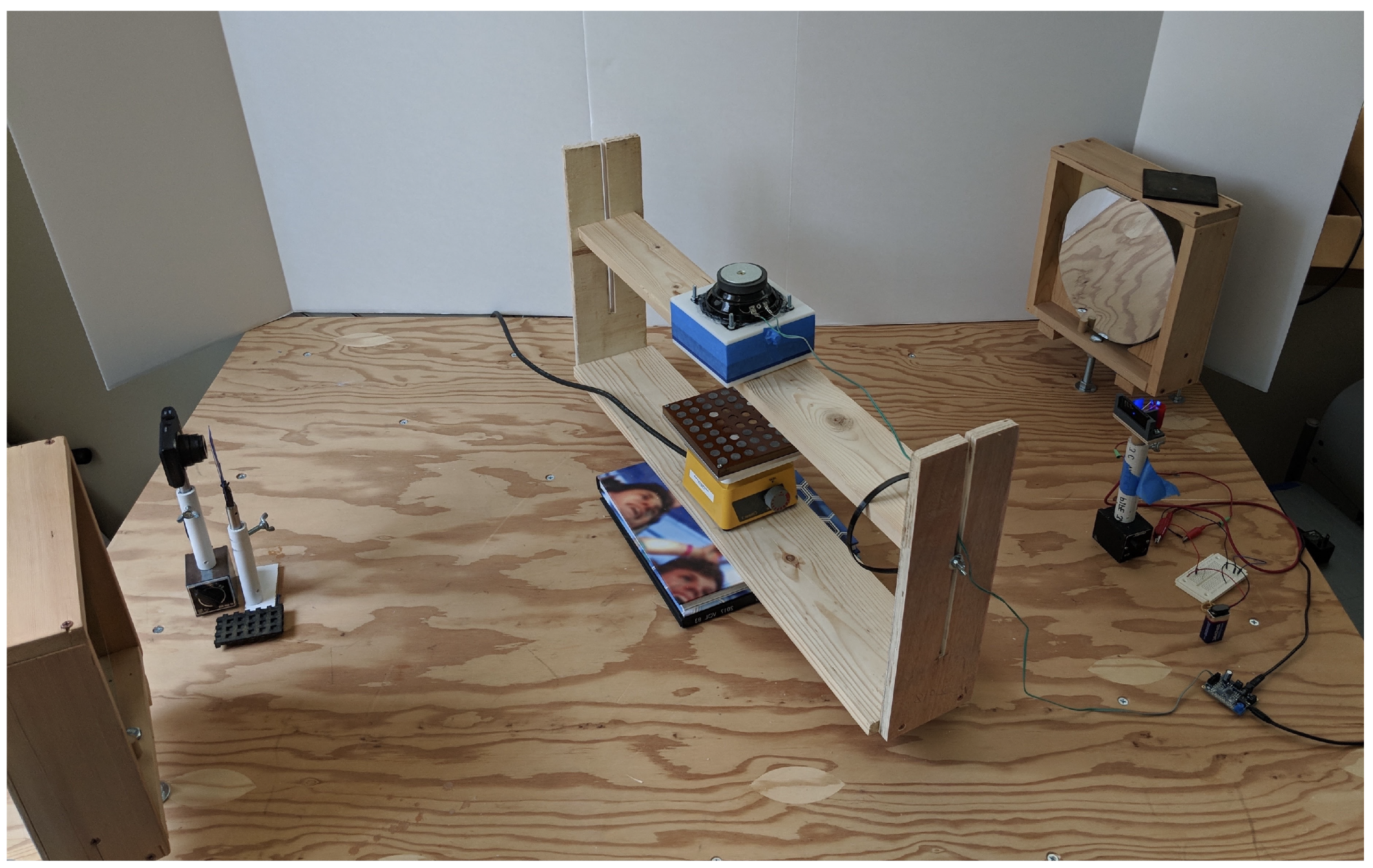
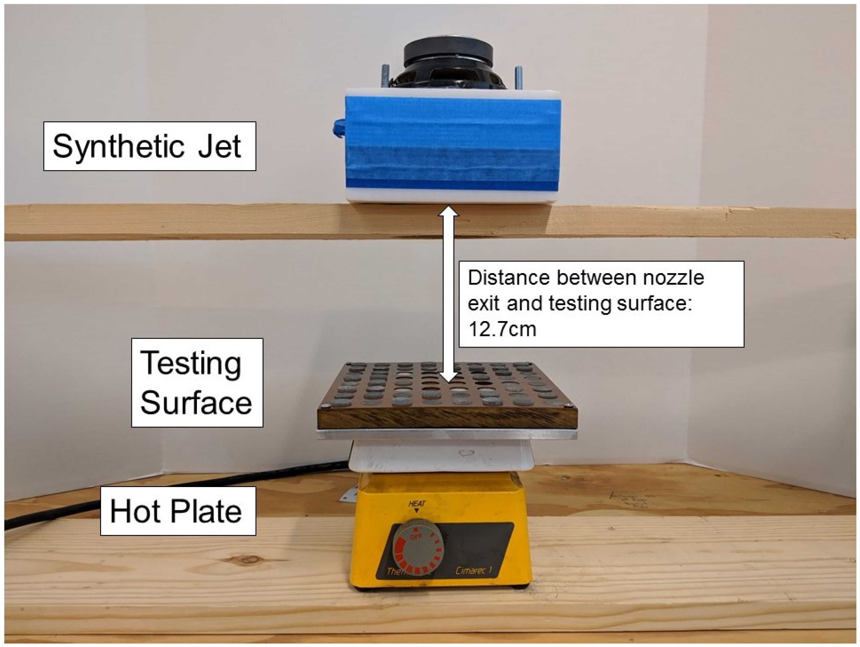
For the second Schlieren experiment, the jet was photographed in a downflow condition impinging on a heated plate. The space between the jet exit and the heated plate was 12.7 cm, a distance selected based on guidance from the electronic cooling applications. The top of the plate was made up of different metal cylinders with uniform spacing to simulate the surface of an electronic device. The heated plate was allowed to reach the steady state, and then, the infrared camera was used to capture the temperature profile of the plate. The jet was activated at a 20–100 Hz frequency and recorded using the high-speed camera. This system is shown in Figure 3.
3.4. Smoke Methods
To capture specific characteristics of the flow from the jet alone, a smoke visualization was performed. The nozzle was placed facing up with a dark background. Using a 50 mm lens, the high-speed camera was used to capture the synthetic jet. Smoke was provided using a smoke machine with tubing connected to the side of the nozzle. This setup was also used to calibrate POD and estimate the jet velocity.
4. Computational Methods
4.1. Frequency Analysis
To determine velocity and confirm the frequency, f, of the synthetic jet, the diameter of the smoke plume passing two fixed vertical points was analyzed. The video was converted to black and white in MATLAB. The smoke plume was primarily white, making it easy to identify relative to the dark background. The next step in the analysis was to collect all the color values of pixels in both fixed row vectors of each frame. The color pixels were on a scale of 0 to 255 with black equaling 0 and white equaling 255. A tolerance of pixel color values larger than 150 was set in order to only count the white pixels of the smoke plume. The threshold of 150 was determined from the calculation of pixel differences in the image. This scaled the vector to only the pixels that made up the smoke plume. Calculating the length of this vector produced the number of pixels that made up the smoke plume. The diameter was then found in units of centimeters using the set pixel conversion factor determined from measuring a known width in the video.
This analysis was completed for each frame in the video. The frame vector was converted to units of seconds using the frame rate conversion factor. The smoke plume diameter was then plotted for each respective row vector over the calculated time span of the video. The maximum diameter change over time was used to estimate the jet velocity near the exit.
4.2. POD Analysis
Proper Orthogonal Decomposition (POD) is based on the diagonalization of a matrix. The mathematical procedure linearly transforms the number of possibly correlated variables into a smaller number of uncorrelated variables. The first component contains as much of the variation in the system as possible. In this case, the matrix X is an matrix composed of multiple observation frames from a video in time.
For the POD analysis, the data were centered by the mean of each row. Then, the covariance matrix was calculated. The covariance matrix is a square, symmetric matrix, whose diagonal represents the variance of particular measurements.
Singular Value Decomposition (SVD) was used to diagonalize the matrix. The SVD diagonalization is shown in Equation (2), where is unitary, is unitary, and is diagonal.
POD gives us a way to quantify the structures that we observe in the flow field of the jet. Each mode of POD is a characteristic of the flow field. Proper orthogonal decomposition was applied to the matrix from the videos, and the energy associated with each of the eigenvalues and eigenvectors was calculated.
The image analysis of the synthetic jets followed a standard approach. First, the video file was imported into MATLAB as a series of images. Each image file was converted to grayscale, and each pixel value became a number in a matrix for each image. The matrix for each frame of the video was reshaped to become one long row of data. The image matrices were then combined to form one large matrix that represents both time and space dimensions, X.
5. Results
5.1. Experimental Results
Figure 4 shows one cycle of the synthetic jet at 20 Hz using the smoke visualization. Figure 5 shows the same frequency for the jet using the Schlieren visualization. The first three images of each set show the major jet, which was a result of the membrane moving towards the exit. In the fourth image, some of the working fluid is being pulled back into the nozzle as the membrane moves away from the exit. An unexpected observation was the formation of a secondary minor jet, the fifth image in each set. This minor jet was small, but not well defined, and only existed for around 3–4 in vertically (7.62–10.16 cm).
For the experiments using the heated plate, the plume created by the jet was tight and easily visualized with the density gradient of the Schlieren. It was experimentally determined with trial and error that the optimal distance to place the jet away from the testing surface was 5 in (12.7 cm), or a distance of , with r defined as the side length of the square exit on the nozzle.
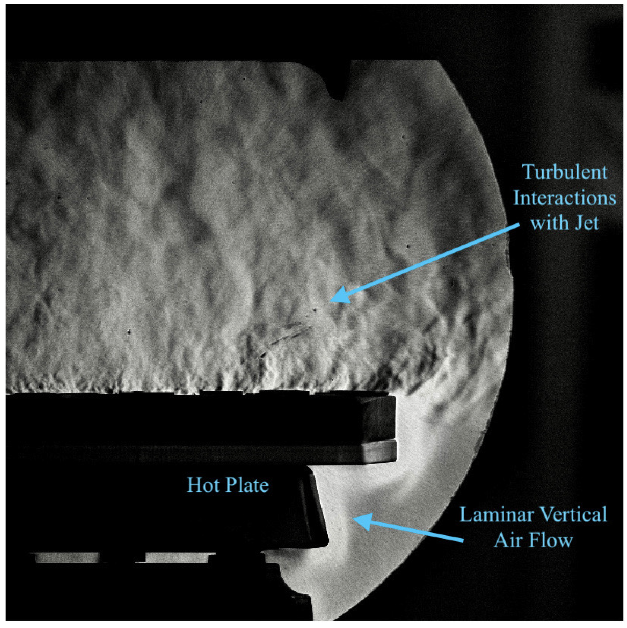
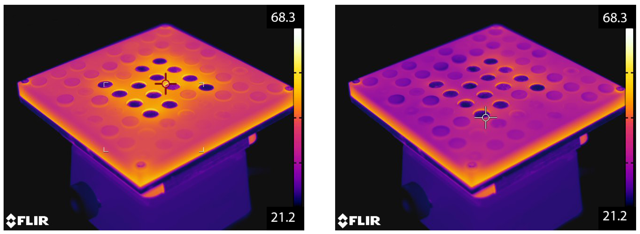
At frequencies ranging from 20–100 Hz, there was significant fluid movement as a result of the synthetic jet. For the jet at 20 Hz, the Schlieren images and infrared images are shown in Figure 6 and Figure 7. The steady-state figure for 20Hz was labeled to show the region of laminar natural convection below the plate where the jet was not interacting significantly. Above the heated plate, the complex mixing of the jet with the air created a turbulent region, cooling the plate. Figure 7 shows that the center of the plate was initially warmer due to the metal cylinders in the center of the plate. After the jet was activated, the temperature of the plate became more uniform as the jet distributed the heat and cooled the surface.
The greatest fluid movement (250 ft/min (11.94 m/s)) and cooling effect (approximately 50 F (10 C) in 60 s) was found at 80Hz, as shown in Figure 8 and Figure 9. The infrared images show significant cooling when compared to the same time period for the 20 Hz jet (Figure 7). Above 100 Hz, fluid movement was insignificant, and therefore, no tests were run above that frequency. A more formal study of this relationship is planned for future work.
5.2. Frequency Analysis Results
The frequency plots created by implementing the MATLAB algorithm represent the true frequency of 20 Hz, as shown in Figure 10. The peaks show where the smoke plume diameter was the largest and passed by the designated pixel row in the video. Each peak was indexed within the MATLAB code. As seen in the plots, the primary peaks for both measurement locations (1 cm and 2 cm) were separated by 0.05 s, or a frequency of approximately 20 Hz. Smaller peaks show the negative flow of the jet as the smoke returns back toward the surface.
The velocity of the smoke plume was estimated using the same method. The calculation was repeated at a distance of 1 cm, and the time for the maximum diameter to travel was calculated. Near the exit of the jet, the velocity estimate was approximately 9 m/s.
5.3. POD Analysis Results
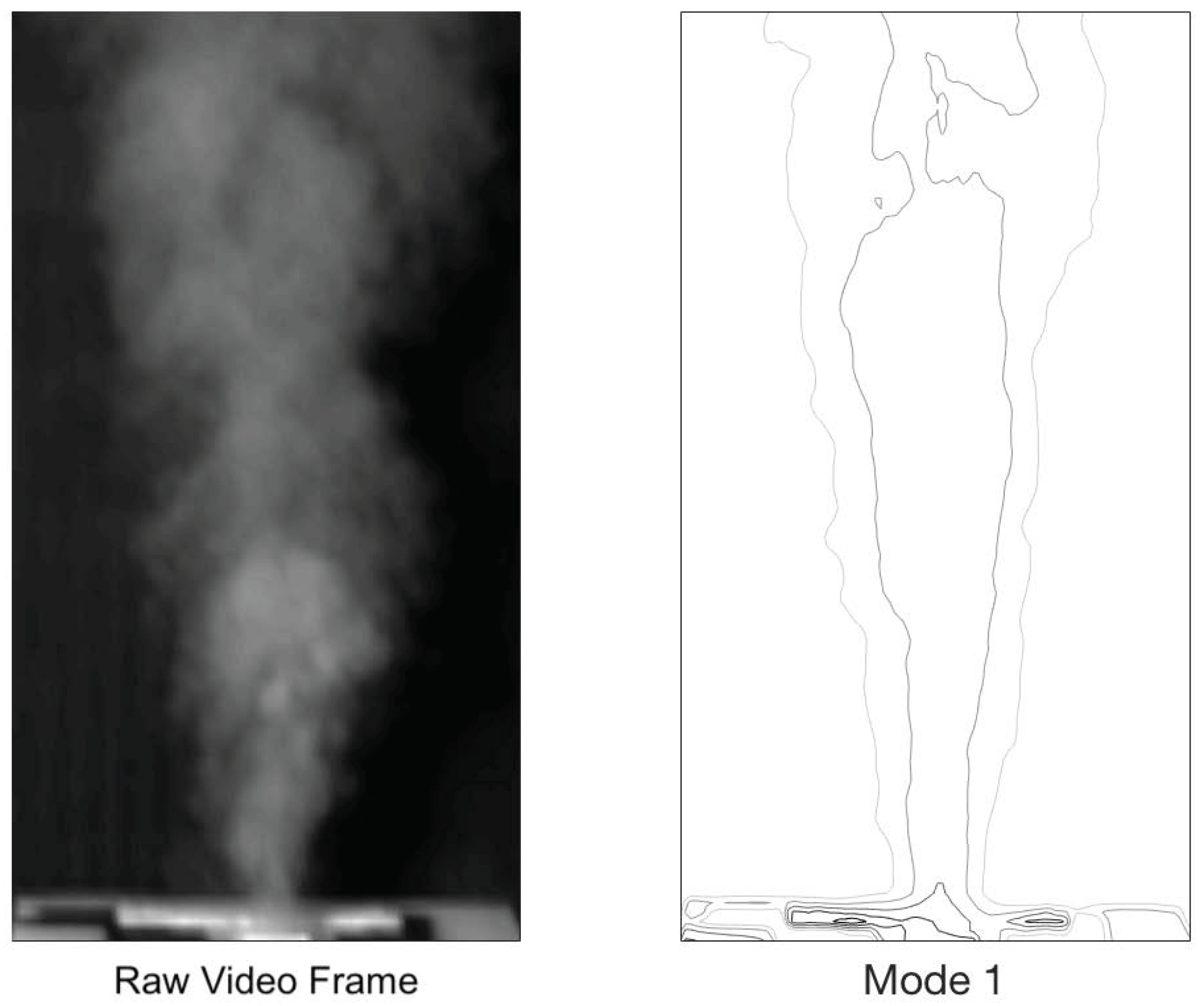
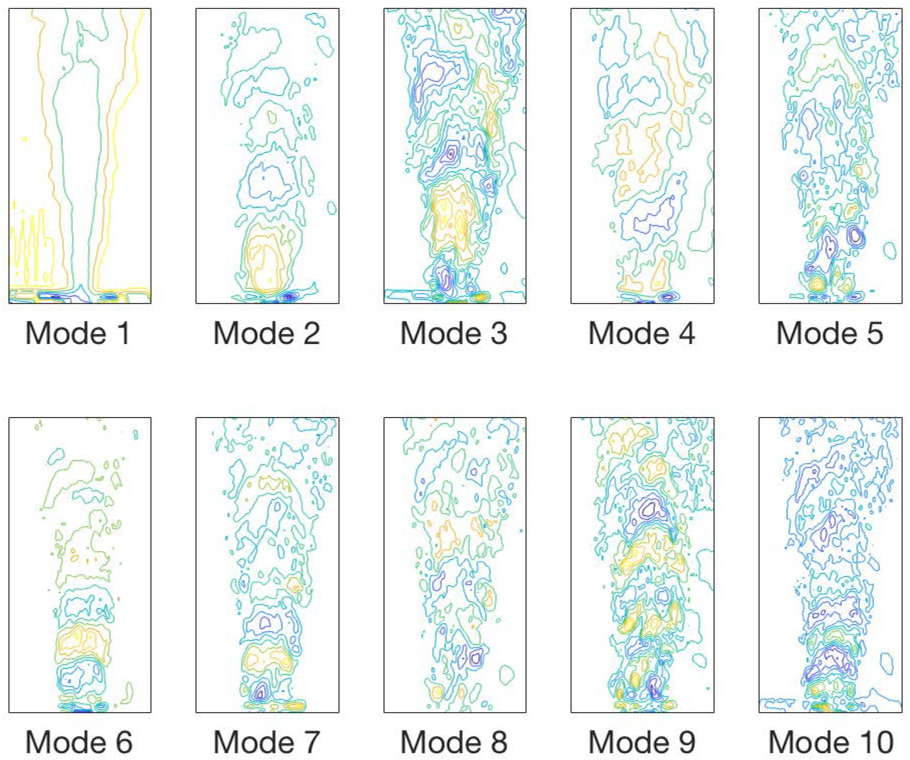
One smoke video was processed using proper orthogonal decomposition for the full length of the video (approximately three cycles of the jet). Figure 11 compares the first mode, which contains the basic structural elements of the flow with a sample frame from the video. Figure 12 shows the first 10 modes of the POD analysis. In each mode, important flow structures are shown. For example, Modes 5, 6, and 7 each show vortex structures, and Mode 6 shows the repeated patterns associated with the synthetic flow.
When using POD, many systems are well characterized mathematically when the modes capture 90% of the energy in the system [3]. For most systems, this is less than 10 modes; however, for the synthetic jet at 80 Hz, 27 modes were required to reach the 90% energy threshold. This indicates that the flow in the system is complex and requires additional modes to characterize it well mathematically. This was expected for the transient version of a synthetic jet. The first five modes and the energy are shown in Table 3 for the smoke jet at 80 Hz.
The same technique was then applied to the more complex flow where the jets were impinging on the heated plate. In this case, the modes required were significantly higher, with 200–239 modes required to reach the same 90% threshold. These values confirmed that the flow was erratic and high in movement, which enhanced the cooling. The results are shown in Table 4 and Table 5. The highest number of modes required was for the 80 Hz frequency, also found to represent the highest heat transfer for the system. This confirmed the trend expected for a more turbulent flow.
6. Discussion
The research team designed a synthetic jet for cooling and then optimized the thermal performance of the synthetic jet. We then tested the best low-cost visualization methods to quantify the flow behaviors. Smoke visualization works well, but has limitations in capturing the complex interaction of the heat transfer and the fluid. The smoke visualization method does offer more opportunities for the calculation of the frequency and velocity in a single jet. The Schlieren visualization was determined to be the best way to visualize the synthetic jet during cooling, since the density gradient visualization captures the influence of the heat transfer. The method also captures more subtle elements of the flow structure, as shown in Figure 5. Schlieren methods were also used to successfully capture the characteristic behavior in a single jet.
The frequency calculation (Figure 10) confirmed peaks spaced out by 0.05 s in both pixel rows of the video where data were taken. This matches the 20 Hz frequency that the modeled cooling jet was pulsed at through the testing iterations. It can be concluded that using this form of video analysis to determine or confirm the frequency is very effective. A limitation of this method is that it requires the pixel row data to be taken a small distance away from where the jet exits the nozzle to avoid visual interference. This allows some time for the fluid to interact with its surroundings, which may have added viscous or drag forces. This could introduce error in the timing of when the smoke plume passes the row where data are collected as compared to the actual frequency at which the jet is pulsating. In general, this type of photography is a low-cost way to determine the jet performance in some applications.
7. Conclusions
At 80 Hz, the plate experienced optimal cooling by the synthetic jet. This frequency of the system represents a more complex optimal than often considered in synthetic jets since the scale of the device and cooling object influences the behavior of the system rather than just the device frequency. This makes characterizing the fluid behavior using POD an important part of the study.
Proper orthogonal decomposition was used to analyze the jet behavior in free air and during cooling applications. POD provides a way to quantify the complexity of the synthetic jet flow for electronic cooling applications. A high number of POD modes to quantify the system indicates a more complex flow. The optimal cooling of the plate occurred at 80 Hz, also the conditions that required the highest number of modes to reach the 90% threshold.
We considered smoke and Schlieren methods with analysis methods for low-cost visualization. We tested each method and quantified the results using proper orthogonal decomposition. Both visualization tools represent a low-cost and efficient way to optimize a synthetic jet application, but the Schlieren method we found to be more robust coupled with the analysis methods.
The results indicated that POD may be used to quantify the relative complexity of a synthetic jet. In future work, this could be used to more fully optimize the frequency of the synthetic jet for cooling and the placement of the synthetic jet. We also confirmed that Schlieren methods would be preferred for the study of jets since including the density information is helpful to optimize the system.
Author Contributions
Experimental work by J.E.P. and W.S. Design of the nozzle, writing, data analysis, and writing—draft preparation by J.E.P. Frequency analysis, writing, and draft preparation by W.S. Conceptualization, methodology, POD analysis, writing, review, editing, supervision, project administration, and funding acquisition by H.E.D. All authors have read and agreed to the published version of the manuscript.
Funding
This research was funded in part by W.M. Keck Foundation.
Institutional Review Board Statement
Not applicable.
Informed Consent Statement
Not applicable.
Data Availability Statement
Videos available from authors upon request.
Acknowledgments
Special thanks to Jared Reese and Jacob Amos for technical support. Thanks to Steve Solovitz for the discussion and suggestions.
Conflicts of Interest
The authors declare no conflict of interest.
Abbreviations
The following abbreviations are used in this manuscript:
| The covariance matrix | |
| f | Frequency |
| POD | Proper Orthogonal Decomposition |
| r | Side length of the square exit on the nozzle |
| SVD | Singular-Value Decomposition |
| t | Time |
| v | Velocity |
| X | The matrix of spatial and temporal data |
References
- Smith, B.L.; Swift, G.W. A comparison between synthetic jets and continuous jets. Exp. Fluids 2003, 34, 467–472. [Google Scholar] [CrossRef]
- Sirovich, L. Turbulence and the dynamics of choerent structures. Q. Appl. Math. 1987, 45, 561–590. [Google Scholar] [CrossRef] [Green Version]
- Dillon, H.E.; Emery, A.F.; Mescher, A.M.; Sprenger, O.; Edwards, S.R. Chaotic Natural Convection in an Annular cavity with non-isothermal walls. Front. Heat Mass Transf. 2011, 2. [Google Scholar] [CrossRef]
- Dillon, H.E.; Emery, A.F.; Mescher, A.M. Analysis of Chaotic Natural Convection in a Tall Rectangular Cavity with Non-Isothermal Walls. Front. Heat Mass Transf. (FHMT) 2013, 4. [Google Scholar] [CrossRef] [Green Version]
- Glezer, A.; Amitay, M. Synthetic Jets. Annu. Rev. Fluid Mech. 2002, 34, 503–529. [Google Scholar] [CrossRef]
- Kercher, D.S.; Lee, J.B.; Brand, O.; Allen, M.G.; Glezer, A. Microjet cooling devices for thermal management of electronics. IEEE Trans. Components Packag. Technol. 2003, 26, 359–366. [Google Scholar] [CrossRef]
- Yi, S.J.; Kim, M.; Kim, D.; Kim, H.D.; Kim, K.C. Transient temperature field and heat transfer measurement of oblique jet impingement by thermographic phosphor. Int. J. Heat Mass Transf. 2016, 102, 691–702. [Google Scholar] [CrossRef]
- Travnicek, Z.; Tesar, V. Annular synthetic jet used for impinging flow mass-transfer. Int. J. Heat Mass Transf. 2003, 46, 3291–3297. [Google Scholar] [CrossRef] [Green Version]
- Pavlova, A.; Amitay, M. Electronic Cooling Using Synthetic Jet Impingement. J. Heat Transf. 2006, 128, 897. [Google Scholar] [CrossRef]
- Arik, M. Local Heat Transfer Coefficients of a High-Frequency Synthetic Jet during Impingement Cooling over Flat Surfaces. Heat Transf. Eng. 2008, 29, 763–773. [Google Scholar] [CrossRef]
- Chaudhari, M.; Puranik, B.; Agrawal, A. Heat transfer characteristics of synthetic jet impingement cooling. Int. J. Heat Mass Transf. 2010, 53, 1057–1069. [Google Scholar] [CrossRef]
- Bazdidi-Tehrani, F.; Karami, M.; Jahromi, M. Unsteady flow and heat transfer analysis of an impinging synthetic jet. Heat Mass Transf. 2011, 47, 1363–1373. [Google Scholar] [CrossRef]
- Bidan, G.; Vézier, C.; Nikitopoulos, D.E. Study of Unforced and Modulated Film-Cooling Jets Using Proper Orthogonal Decomposition—Part I: Unforced Jets. J. Turbomach. 2012, 135, 021037. [Google Scholar] [CrossRef]
- Bidan, G.; Vézier, C.; Nikitopoulos, D.E. Study of Unforced and Modulated Film-Cooling Jets Using Proper Orthogonal Decomposition—Part II: Forced Jets. J. Turbomach. 2012, 135, 021038. [Google Scholar] [CrossRef]
- Ghaffari, O.; Solovitz, S.A.; Ikhlaq, M.; Arik, M. An investigation into flow and heat transfer of an ultrasonic micro-blower device for electronics cooling applications. Appl. Therm. Eng. 2016, 106, 881–889. [Google Scholar] [CrossRef] [Green Version]
- Ghadi, S.; Esmailpour, K.; Hosseinalipour, S.; Mujumdar, A. Experimental study of formation and development of coherent vortical structures in pulsed turbulent impinging jet. Exp. Therm. Fluid Sci. 2016, 74, 382–389. [Google Scholar] [CrossRef]
- Albright, S.O.; Solovitz, S.A. Examination of a Variable-Diameter Synthetic Jet. J. Fluids Eng. 2016, 138, 121103. [Google Scholar] [CrossRef]
- Firdaus, S.M.; Abdullah, M.Z.; Abdullah, M.K.; Mazlan, A.Z.A.; Ripin, Z.M.; Amri, W.M.; Yusuf, H. Synthetic Jet Study on Resonance Driving Frequency for Electronic Cooling. In Regional Conference on Science, Technology and Social Sciences (RCSTSS 2016); Springer: Singapore, 2018; pp. 435–443. [Google Scholar] [CrossRef]
- Solovitz, S.A.; Ghaffari, O.; Arik, M. FREQUENCY-DEPENDENT FLOW RESPONSE OF A HIGH-SPEED RECTANGULAR SYNTHETIC JET. J. Flow Vis. Image Process. 2016, 23, 93–116. [Google Scholar] [CrossRef]
- Viggiano, B.; Dib, T.; Ali, N.; Mastin, L.G.; Cal, R.B.; Solovitz, S.A. Turbulence, entrainment and low-order description of a transitional variable-density jet. J. Fluid Mech. 2018, 836, 1009–1049. [Google Scholar] [CrossRef] [Green Version]
- Kristo, P.J.; Kimber, M.L.; Girimaji, S.S. Towards Reconstruction of Complex Flow Fields Using Unit Flows. Fluids 2021, 6, 255. [Google Scholar] [CrossRef]
- Li, J.; Liu, J.; Pei, J.; Mohanarangam, K.; Yang, W. Experimental study of human thermal plumes in a small space via large-scale TR PIV system. Int. J. Heat Mass Transf. 2018, 127, 970–980. [Google Scholar] [CrossRef]
- Albright, S.O.; Solovitz, S.A. Development of a Variable Diameter Synthetic Jet Actuator. In Advances in Aerospace Technology; ASME: New York, NY, USA, 2014; Volume 1, p. V001T01A002. [Google Scholar] [CrossRef]
- Kaessinger, J.C.; Kors, K.C.; Lum, J.S.; Dillon, H.E.; Mayer, S.K. Utilizing Schlieren Imaging to Visualize Heat Transfer Studies. In Proceedings of the American Society of Mechanical Engineers 2014 International Mechanical Engineering Conference, Montreal, QC, Canada, 14–20 November 2014; pp. 2014–38329. [Google Scholar] [CrossRef]
Figure 1.
Schematic drawing of the assembled nozzle.

Figure 2.
Schematic drawing and photograph of the experimental Schlieren configuration.


Figure 3.
Photograph of the experimental setup for the heated plate test.

Figure 4.
Smoke machine, 20 Hz, 3500 fps. Exported at 2× speed.

Figure 5.
Schlieren, 20 Hz, 3500 fps. Exported at 2× speed.

Figure 6.
Schlieren image showing the steady-state interaction of air from the synthetic jet with a hot testing surface, 20 Hz.
Figure 6.
Schlieren image showing the steady-state interaction of air from the synthetic jet with a hot testing surface, 20 Hz.

Figure 7.
Infrared photo of the hot testing surface at time 0 s and then 60 s with a jet at 20 Hz. The temperature scale is C.
Figure 7.
Infrared photo of the hot testing surface at time 0 s and then 60 s with a jet at 20 Hz. The temperature scale is C.

Figure 8.
Schlieren image showing the steady-state interaction of air from the synthetic jet with the hot testing surface, 80 Hz.
Figure 8.
Schlieren image showing the steady-state interaction of air from the synthetic jet with the hot testing surface, 80 Hz.

Figure 9.
Infrared photo of the hot testing surface at time 0 s and then 60 s with a jet at 80 Hz. The temperature scale is C.
Figure 9.
Infrared photo of the hot testing surface at time 0 s and then 60 s with a jet at 80 Hz. The temperature scale is C.

Figure 10.
Diameter of the jet over time for two vertical locations. The spacing of the largest peaks (both 1 cm and 2 cm from the exit) are both approximately 0.05 s, near 20 Hz.
Figure 10.
Diameter of the jet over time for two vertical locations. The spacing of the largest peaks (both 1 cm and 2 cm from the exit) are both approximately 0.05 s, near 20 Hz.

Figure 11.
The first mode (right) of the POD of the jet operating at 80 Hz captures key characteristics of the flow when compared with the raw video frames (left).
Figure 11.
The first mode (right) of the POD of the jet operating at 80 Hz captures key characteristics of the flow when compared with the raw video frames (left).

Figure 12.
The first 10 modes of the POD of the jet operating at 80 Hz.


Table 1.
Summary of experimental and computational work on jets.
| Citation | Year | Frequency | Jet Type | Study Type |
|---|---|---|---|---|
| (Hz) | ||||
| Kercher et al. [6] | 2003 | 1–1000 | synthetic | |
| Travnicek and Tesar [8] | 2003 | 106–692 | synthetic | smoke |
| Smith and Swift [1] | 2003 | synthetic and | Schlieren | |
| continuous | ||||
| Pavlova et al. [9] | 2006 | 420–1200 | synthetic | |
| Arik [10] | 2008 | 4500 | synthetic | |
| Chaudhari et al. [11] | 2009 | 100–350 | synthetic | |
| Bazdidi-Tehrani et al. [12] | 2011 | 16–400 | synthetic | |
| Biden et al. [13] | 2012 | unforced jet | POD | |
| in crossflow | ||||
| Biden et al. [14] | 2012 | forced jet | POD | |
| in crossflow | ||||
| Ghaffari et al. [15] | 2016 | 20,000 | ultrasonic | |
| microblower | ||||
| Ghadi et al. [16] | 2016 | pulsed | smoke | |
| impinging jet | ||||
| Albright and Solovitz [17] | 2016 | variable-diameter | ||
| synthetic jet | ||||
| Firdaus et al. [18] | 2018 | 300–700 | synthetic | |
| Solovitz et al. [19] | 2018 | 350–2000 | synthetic | PIV |
| Viggiano et al. [20] | 2018 | variable-density | POD and PIV | |
| jet | ||||
| Kristo et al. [21] | 2021 | crossflow jets | POD and PIV | |
| Present work | 2021 | 20–100 | synthetic | POD, smoke, |
| Schlieren |
Table 2.
Summary of the equipment used in the experiments.
| Description | Model |
|---|---|
| Canon DSLR | EOS 7D Mark II (G) |
| Camera Lens | EF100/2.8 L |
| MACRO IS USM | |
| FLIR IR Camera | |
| PHANTOM Hi-Speed Camera | V711 |
| Canon Point and Shoot | PowerShot |
| ELPH 300 HS | |
| Smoke Machine | |
| 4” Speaker | Sony Xplod |
| XS-GTF1027 | |
| Amplifier | Adafruit Stereo 20 W |
| Class D Amplifier | |
| 10 mm Blue LEDs | |
| Hot Plate | Thermolyne HP46515 |
| Multimeter | RSR MAS830 |
| Thermocouple | FLUKE 80TK |
| Thermocouple probe | FLUKE |
| Wane Anemometer | Fieldpiece EHdl1 |
Table 3.
Energy associated with the modes developed from the POD at 80 Hz for the synthetic jet in smoke.
Table 3.
Energy associated with the modes developed from the POD at 80 Hz for the synthetic jet in smoke.
| Mode | Eigenvalue | Total Energy |
|---|---|---|
| % | ||
| 1 | 114.64 | 44.46 |
| 2 | 18.23 | 7.07 |
| 3 | 15.92 | 6.17 |
| 4 | 14.48 | 5.62 |
| 5 | 8.31 | 3.22 |
| 27 | 0.96 | 0.37 |
Table 4.
Energy associated with the modes developed from the POD at 20 Hz for the jet on the heated plate with the Schlieren.
Table 4.
Energy associated with the modes developed from the POD at 20 Hz for the jet on the heated plate with the Schlieren.
| Mode | Eigenvalue | Total Energy |
|---|---|---|
| % | ||
| 1 | 480.74 | 15.76 |
| 2 | 99.83 | 3.27 |
| 3 | 80.12 | 2.62 |
| 4 | 73.41 | 2.41 |
| 5 | 64.07 | 2.10 |
| 200 | 2.82 | 0.09 |
Table 5.
Energy associated with the modes developed from the POD at 80 Hz for the jet on the heated plate with the Schlieren.
Table 5.
Energy associated with the modes developed from the POD at 80 Hz for the jet on the heated plate with the Schlieren.
| Mode | Eigenvalue | Total Energy |
|---|---|---|
| % | ||
| 1 | 433.65 | 14.27 |
| 2 | 98.70 | 3.25 |
| 3 | 82.12 | 2.70 |
| 4 | 67.73 | 2.23 |
| 5 | 52.27 | 1.72 |
| 239 | 2.85 | 0.09 |
Publisher’s Note: MDPI stays neutral with regard to jurisdictional claims in published maps and institutional affiliations. |
© 2021 by the authors. Licensee MDPI, Basel, Switzerland. This article is an open access article distributed under the terms and conditions of the Creative Commons Attribution (CC BY) license (https://creativecommons.org/licenses/by/4.0/).
Share and Cite
MDPI and ACS Style
Pellessier, J.E.; Dillon, H.E.; Stoltzfus, W. Schlieren Flow Visualization and Analysis of Synthetic Jets. Fluids 2021, 6, 413. https://0-doi-org.brum.beds.ac.uk/10.3390/fluids6110413
AMA Style
Pellessier JE, Dillon HE, Stoltzfus W. Schlieren Flow Visualization and Analysis of Synthetic Jets. Fluids. 2021; 6(11):413. https://0-doi-org.brum.beds.ac.uk/10.3390/fluids6110413
Chicago/Turabian StylePellessier, John E., Heather E. Dillon, and Wyatt Stoltzfus. 2021. "Schlieren Flow Visualization and Analysis of Synthetic Jets" Fluids 6, no. 11: 413. https://0-doi-org.brum.beds.ac.uk/10.3390/fluids6110413