
Predictions of Vortex Flow in a Diesel Multi-Hole Injector Using the RANS Modelling Approach


Department of Engineering, Mechanical Engineering and Aeronautics, City, University of London, Northampton Square, London EC1V 0HB, UK
*
Author to whom correspondence should be addressed.
Fluids 2021, 6(12), 421; https://0-doi-org.brum.beds.ac.uk/10.3390/fluids6120421
Submission received: 20 October 2021
/
Revised: 12 November 2021
/
Accepted: 16 November 2021
/
Published: 23 November 2021
(This article belongs to the Collection Advances in Turbulence)
Abstract
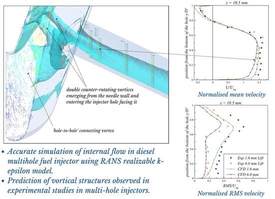
:The occurrence of vortices in the sac volume of automotive multi-hole fuel injectors plays an important role in the development of vortex cavitation, which directly influences the flow structure and emerging sprays that, in turn, influence the engine performance and emissions. In this study, the RANS-based turbulence modelling approach was used to predict the internal flow in a vertical axis-symmetrical multi-hole (6) diesel fuel injector under non-cavitating conditions. The project aimed to predict the aforementioned vortical structures accurately at two different needle lifts in order to form a correct opinion about their occurrence. The accuracy of the simulations was assessed by comparing the predicted mean axial velocity and RMS velocity of LDV measurements, which showed good agreement. The flow field analysis predicted a complex, 3D, vortical flow structure with the presence of different types of vortices in the sac volume and the nozzle hole. Two main types of vortex were detected: the “hole-to-hole” connecting vortex, and double “counter-rotating” vortices emerging from the needle wall and entering the injector hole facing it. Different flow patterns in the rotational direction of the “hole-to-hole” vortices have been observed at the low needle lift (anticlockwise) and full needle lift (clockwise), due to their different flow passages in the sac, causing a much higher momentum inflow at the lower lift with its much narrower flow passage.
1. Introduction
The emergence of direct injection technology has significantly improved IC engines in terms of performance, efficiency, and emissions [1]. Direct injection technology usually uses multi-hole fuel injectors due to their geometrical flexibility, which operate at high pressures over a very short duration. This ensures the injection of precise amounts of fuel into the combustion chamber for different combustion strategies. However, such massive fuel acceleration in such a small period within the narrow passages of the injector leads to the development of localised regions or pockets of low liquid pressure. When the local pressure in these pockets becomes lower than the saturation pressure of the liquid, it results in the occurrence of voids or cavities within the liquid—this process is called cavitation [2].
The occurrence of cavitation directly influences the emerging spray [3], and the development of cavitating structures in fuel injectors is mainly owed to their geometry. Previous simulations and experimental studies with multi-hole injectors have shown that the main cavitation occurs at the upper edge of the hole entrance of the fuel injector and is known as geometrical cavitation [3,4,5,6,7,8]. This is attributed to the formation of a recirculation region at the upper edge of the hole entrance due to the detachment of the fluid and abrupt reduction in the cross-sectional area, which facilitates liquid acceleration. LDV results of mean axial velocity near the entrance of the injector hole have confirmed the presence of the recirculation regions in multi-hole injectors [4,8]. Experimental observations have shown that cavitation enhances the primary break-up and subsequent atomisation of the liquid due to the perceived enhancement of turbulence, which facilitates mixing, enabling better combustion [3,9,10,11]; the same observations have also shown that cavitation can cause spray instability. Experimental studies on multi-hole injectors have also shown that when the geometrically induced cavitation reaches the injector hole exit, the air from the downstream—with higher local pressure than the fuel vapour pressure—enters the injector hole. This air entrainment replaces the cavitation vapour, leading to the development of PHP (partial hydraulic flip), which further enhances the spray instability [3]. Moreover, cavitating bubbly fluid behaves like a compressible fluid—a phenomenon well explained in the authors’ previous paper [12].
In addition to the main geometrical cavitation, the internal fluid flow in the injector causes the development of complex vortices. When the local pressure at the core of these vortices goes below the vapour pressure, the liquid starts to form cavitation pockets. As explained by Kumar et al. [13], there are two types of such cavitating structures, which have been observed frequently in several experimental studies: The first type is hole-to-hole connecting vortex cavitation, which has been noted as an arc-shaped vortex, connecting two adjacent holes and the recess between the needle and the injector wall. The second observed type of these cavitation structures is a double counter-rotating vortical cavitation structure, originating from the needle wall and entering the opposing injector holes.
The presence of vortical cavitating structures is noticed concurrently in the injector hole with geometrical horseshoe-type cavitating structures. However, such a vortical structure is frequently seen entering the injector at the bottom of the inlet, consequently disrupting the spray [3,9,10,11]. Along with this, vortical cavitating structures are also seen merging with the geometrically induced cavitating structures, further upsetting the desired spray—especially in terms of its stability. The observed cavitating structures in multi-hole injectors are believed to be due to the geometry of the injector’s sac volume and the arrangement of the nozzle holes. Thus, it is very important to have a good understanding of how these vortical structures are formed, which was the prime objective of the present study. Flow field analysis was be performed under non-cavitating flow conditions (very low cavitation numbers; CN ≈ 0.45) in order to identify the mechanisms of the development of these vortices in the fuel injectors, and to identify the differences in their structures at low and full needle lifts. The low lift represents the transient flow conditions during the injection process when the needle is opening or closing; for more details, see Section 2.
Many previous simulations efforts have been made to facilitate a sound understanding of internal flows in multi-hole fuel injectors. LDV (Laserdoppler velocimetry) experimental results have often been used to assess and validate different CFD modelling approaches. Full details are given by the authors in their previous paper [13], and a brief summary is given below. The first such attempt was by Arcoumanis et al. [4], who used their in-house CFD solver to simulate non-cavitating conditions in mini-sac injectors, and achieved reasonably good agreement with experimental measurements of mean velocity and RMS (Root mean square) velocity using a low-resolution mesh. They later included cavitation simulation in their CFD code [14], treating liquid as a continuous phase in the Eulerian frame and cavitation vapour bubbles as a disperse phase (with many submodels), and tracked them in a Lagrangian frame. They checked the validity of their model by comparing predicted mean and RMS velocities with the experimental values, and also by comparing the predicted void fraction with high-speed digital images; both comparisons achieved fairly decent agreements. They further added more features to their dispersed-phase model, such as bubble breakup and coalescence [15]; they assessed their model quantitatively by comparing predicted voids with CT (computed tomography) measurements of the same geometry for the single-hole nozzle, and predicted mean and RMS velocity with LDV measurements for the multi-hole injector, for which they achieved reasonably good accuracy. Papoutsakis et al. [16] also used LDV measurements to validate their CFD results for the multi-hole injector; they performed single-phase simulations and compared RANS (Reynolds-averaged Navier–Stokes) and LES (Large-eddy simulations) predictions with experimental measurements. They achieved comparable results and fairly good agreement with experimental data using both approaches; however, the advantages of one approach over the other in a similar mesh could not be established.
LDV measurements have also been used to assess CFD simulations in single-hole nozzles. Sou et al. [17] performed CFD simulations of cavitating flow in a rectangular single-hole nozzle geometry using in-house LES CFD code, and assessed their predictions by comparing the predicted mean and RMS velocity with LDV results, and cavitation with captured still images. They achieved decent agreement for mean velocity but were far off from experimental values of RMS velocity at positions where cell size was not sufficiently fine. Koukouvinis et al. [18] used the experimental data of Sou et al. to assess their CFD simulations; they performed RANS and LES simulations, achieving more accurate results using the LES method than RANS; however, they could not justify the suitability of LES over RANS, due to the high computational cost of the former. A recent experimental work [19] investigated vortical flow structure in a single-nozzle injector using high-speed combined diffuse backlight illumination and schlieren imaging, and showed that the presence of coherent vortical structures has a measurable influence on the dynamics of the emerging spray, leading to distinct variation in spray cone angle. Meanwhile, the latest CFD simulation [20] showed that the origin of in-nozzle vortex cavitation structures can be traced back to the sac volume and on-needle surface, and that the nonuniformity of the oil viscosity (due to viscous heating) gives rise to vortex formation. LDV data [8] have been recently used by Kumar et al. [13] to assess CFD simulations in a multi-hole fuel injector; they used the RANS modelling approach to approximate turbulence, and the Eulerian–Eulerian cavitation modelling method to reproduce cavitation; they achieved reasonably good agreements with experimental data for mean and RMS velocity with LDV counterparts, and for cavitation structures with experimental high-speed digital images.
The present study focuses on the accurate prediction of flow field structures for non-cavitating conditions at partial (lower) and full needle lifts. This project aims to enrich the research community’s understanding of internal flows in fuel injectors via accurate prediction and thorough analysis of the flow field at low cavitation numbers. Through this case study, we aim to identify the most probable location of cavitation inception in fuel injectors, as we believe this will help engineers and researchers to improve contemporary injector design.
The reference injector geometry [8] for the present simulation was a 20-time replica of a Bosch vertical axis-symmetric fuel injector fixed on a steady-state test rig representing quasi-steady conditions at lower and full needle lifts. We acknowledge that the transient effects of needle opening and closing on the internal flow have not been modelled in this study. Although this transient effect is present for a very short period, it has a huge impact on internal flow structure—especially at high injection pressures with diesel injectors—which influences the near-field emerging spray, atomisation, and combustion. This subject has recently been experimentally investigated by Mamaikin et al. [21], using X-ray imaging. Strotos et al. [22] recently conducted a computational investigation of the transient effects of needle opening and closing; they simulated the effects of transient heating in a high-pressure diesel injector; their study showed that increasing the injection pressure from 2000 to 3000 bar caused a considerable increase in fluid temperature above the boiling point, thus leading to fuel boiling and instability. Nevertheless, as mentioned above, the present study is focused on gaining a fundamental understanding of internal flow in fuel injectors, which requires some features to be kept constant.
For the present case study, two reference cases were simulated, with CN (cavitation number) = 0.44 and Re (Reynolds number) = 18,000 at a low needle lift of 1.6 mm, and CN = 0.45 and Re = 21,000 at full needle lift (6.0 mm), under steady -low conditions; the flow was wall-bounded and non-cavitating. Thus, steady-state RANS appeared to be the most suitable turbulence modelling approach to simulate the aforementioned reference cases, due to its ability to predict such flows efficiently and with sufficient accuracy [23]. Amongst the turbulence models, we opted for a realisable k-epsilon turbulence model [24], as in the author’s previous comparative assessment [25], it was established that the realisable k-epsilon model provided the most accurate prediction for this class (internal flows in multi-hole injectors and nozzles) of flows. Thus, the main contributions of the current research paper are to simulate complex vortical flow within a multi-hole diesel injector using RANS with a realisable k-epsilon turbulence model, in order to validate prediction results with accurate LDV measurements and show the usefulness of the simulation model for such applications; to identify mechanisms of the formation of different types of vortex structures, and their developments that are responsible for the formation of vortex cavitation; and to differentiate the vortical flow field structures at low (1.6 mm) and full (6.0 mm) needle lifts. Details of the flow configuration are provided in the next section, followed by simulation methodology and numerical methods. The results are presented and discussed in the subsequent section, and the paper ends with a summary of the main findings.
2. Flow Configuration
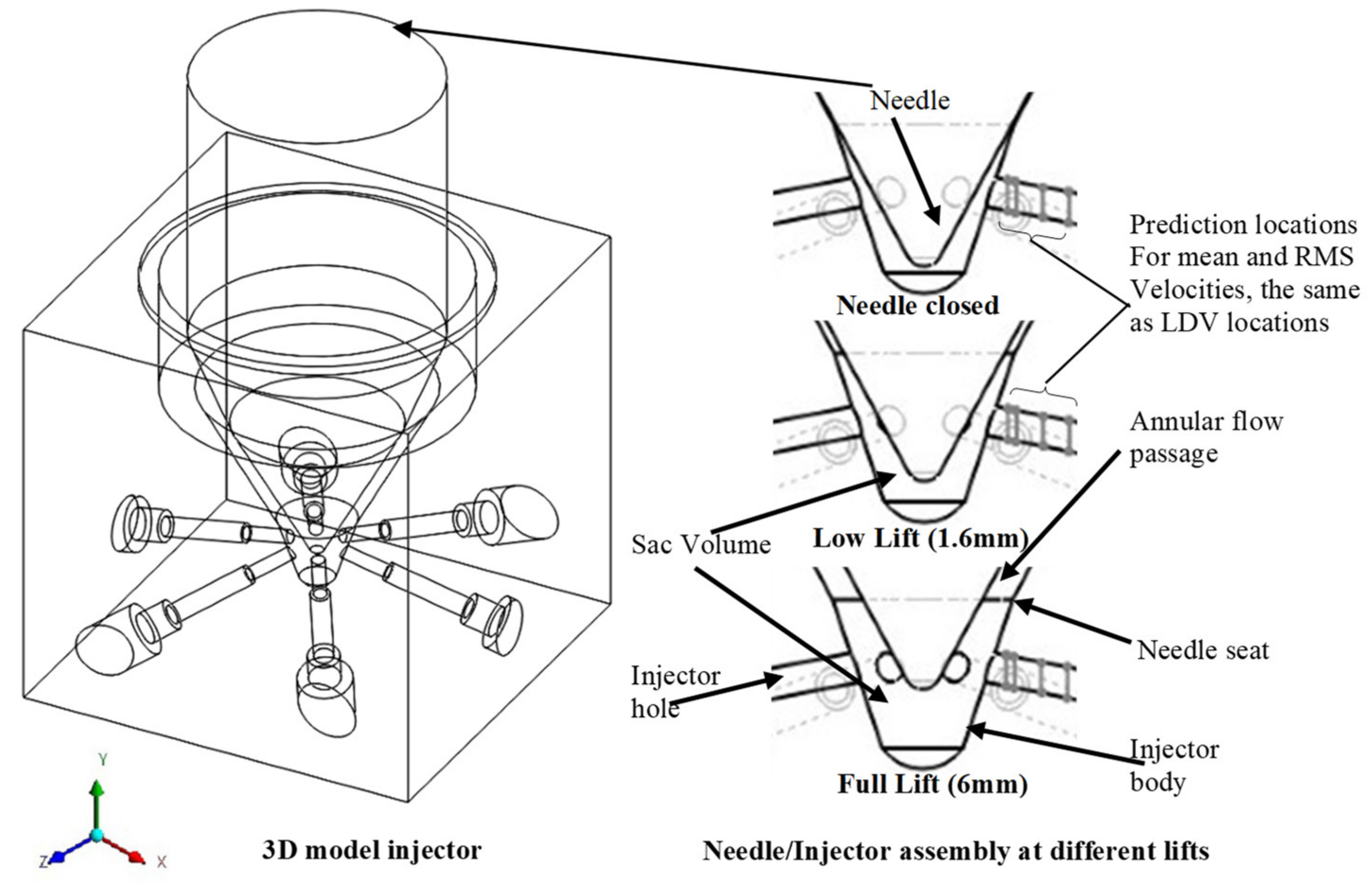
The simulation was conducted on a model injector 20 times larger than the real size, with the same geometry and setup as used by the authors of [8], who performed an extensive experimental work; a summary of the experiment is given below (for more details, see [8,13]). The 3D model geometry represents a multi-hole axisymmetric fuel injector nozzle of a Bosch conical mini-sac type six-hole (60° apart) vertical diesel fuel injector, as shown in Figure 1. The injector/needle assembly for three different needle lifts of full (6 mm), low (1.6 mm), and closed (0.0 mm) is also shown in Figure 1, where the annular flow passage (between the needle and the injector body), sac volume, nozzle, and other key flow features within the mini-sac configuration are highlighted. It should be noted that the needle lift is a measure of offset distance from the needle seat (full shut-off point), and varies from zero—when the needle is at seat position—to full lift, when the needle is fully open. The needle opening/closing durations are very short—around 0.1 ms—and much shorter than the full lift duration (1.0–2.5 ms, depending on engine load). The fuel flow during needle opening/closing events is transient, while at full needle lift it is considered to be steady and stable. The sac volume is a small cavity between the needle seat and the end of the injector, where different vortical flows take place during the injection process, the formation and development of which were the focus of our simulations.
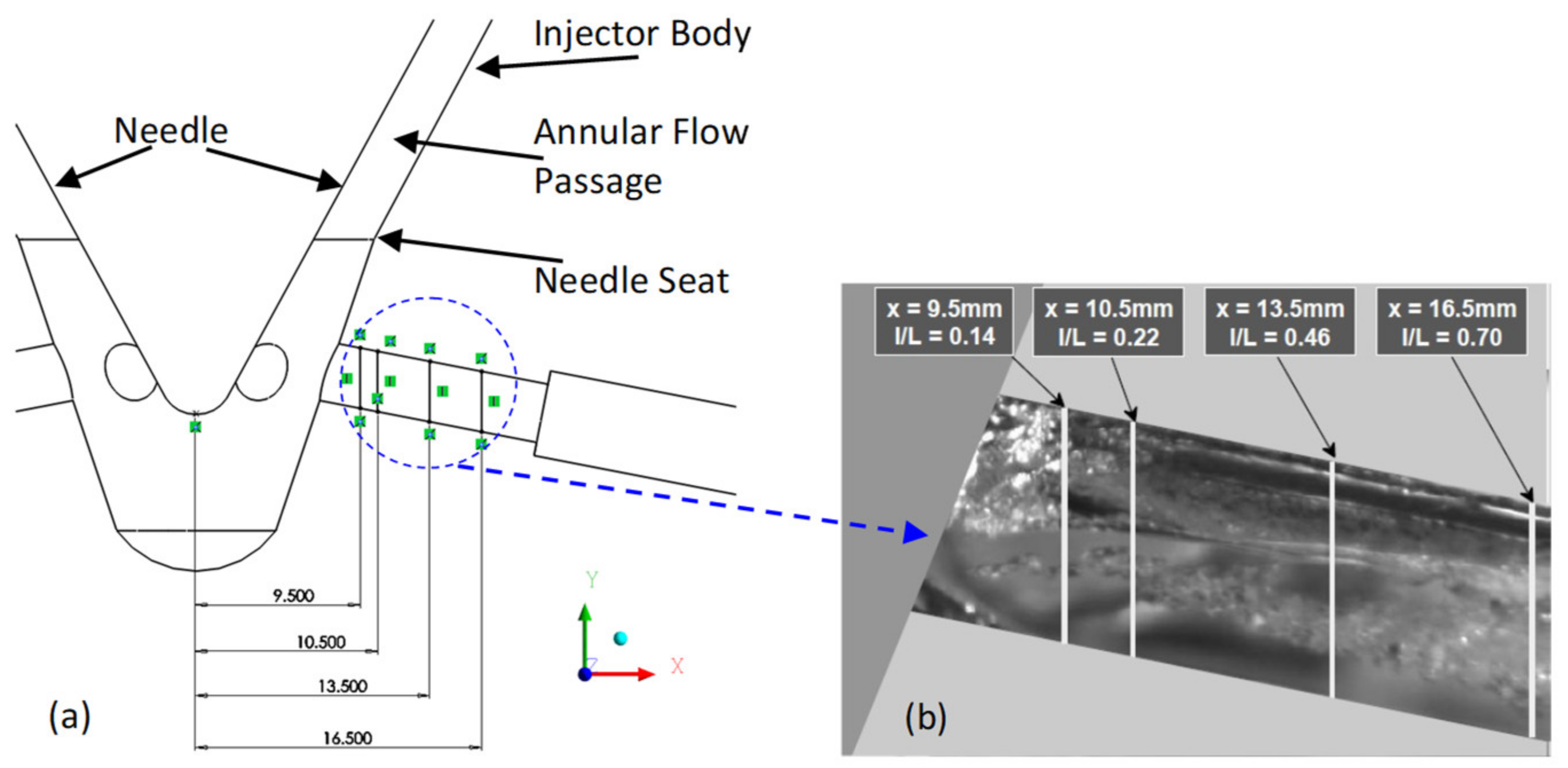
The highlighted prediction locations of mean and RMS velocities on Figure 1 are given in detail in Figure 2a, which are the same locations as those shown in Figure 2b, where the measurements were made, and under the same operating conditions in order to allow for accurate validation of the CFD model. The experimental model was set up on the steady-state test rig (i.e., a fixed needle with no transient movement) to measure axial mean and turbulence velocities at different axial locations within the nozzle hole, and to capture in-nozzle cavitation and its development (Figure 2b) by using a high-speed imaging technique. Additionally, the same working fluid with the same properties as used in the experiment was used for the simulations. The experimental working fluid was a mixture of tetralin (32%) and turpentine (68%) with a density, kinematic viscosity, and vapour pressure of 895 kg/m3, 1.64 × 10⁻⁶ m2/s, and 1 KPa, respectively. The choice of this mixture was to use the refractive index matching technique [26] to ensure that the refractive index of the working fluid was the same as that of the Perspex (the material used to manufacture the model injector) and also to provide full optical access—especially near the walls of the nozzle and the sac volume, with steep curvatures. The operating conditions for the present CFD simulations are listed in Table 1.
3. Methodology
3.1. Governing Equations
Steady-state incompressible RANS (Reynolds-averaged Navier–Stokes) Equations were employed, with the following form:
where is the mean rate of the strain tensor, is the mean fluid velocity in the direction, is the density of the fluid, is the mean pressure, is the dynamic viscosity, is the source term for body forces such as gravity, is the Kronecker delta, which is 1 when = and 0 when , and is the apparent stress owing to the fluctuating velocity field, and is generally referred to as Reynolds stress.
The Reynolds stress in the present study was modelled using Boussinesq approximation, as follows:
which can be shorthanded as:
where k is the turbulent kinetic energy defined by the following equation:
3.2. Turbulence Model
The realisable k-epsilon turbulence model proposed by Shih et al. [24] has the following form:
where is the turbulent kinetic energy, is the turbulent viscosity or eddy viscosity, and is the turbulence dissipation rate, which is defined by the following term:
The following is the transport equation of :
where , , .
The constants are as follows:
The Eddy viscosity is assumed to be isotropic, and is computed using the following equation:
For this to be realisable, the model requires maintaining non-negativity of normal stress, , and “Schwarz inequality” [29,30]. The Schwarz inequality is defined by the following term:
The realisability is achieved by formulating the in Equation (9) by the following equation:
where:
and:
where is the mean rate of the rotation tensor, = , viewed in a moving reference frame with angular velocity . The model constants and are given by:
4. Numerical Methods
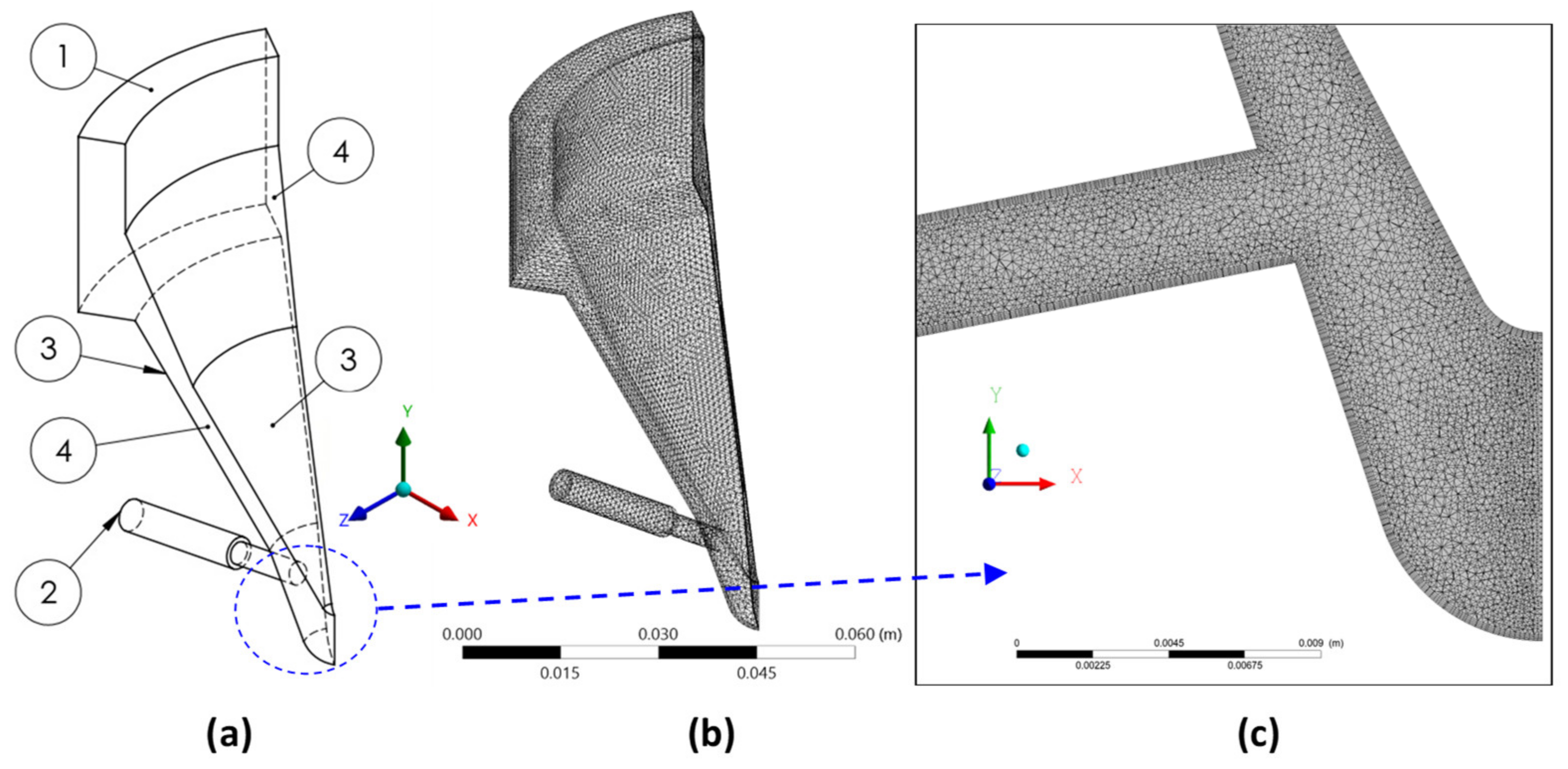
In this study, ANSYS Fluent v14.5 [31] was employed to solve the governing equations using the finite volume method [27]. Since the flow regime is quasi-steady, steady-state simulations were performed, and the pressure–velocity coupling was achieved using the SIMPLE algorithm [32]. Only one-sixth of the flow domain was numerically simulated, due to symmetrical nozzle geometry, so as to reduce computational effort, as shown in Figure 3a. Unstructured grids were used—the same as those of [13], as shown in Figure 3b,c—with tetrahedral cells and five layers of prism cells on the walls in order to accurately resolve near-wall turbulence. The maximum aspect ratio and skewness of all grids were 11.2 and 0.759, respectively.
The mesh convergence was performed until comparable profiles of mean velocity and RMS velocity profiles were achieved, as shown in Appendix A for the low lift; the mesh convergence for the full lift was presented in [13]. Thus, the results of grid 6, with 21,216,968 cells, were used for pre-processing at low needle lift, while grid 2, with 13,016,832 cells, was used for the full needle lift. The turbulence was modelled using the realisable k-epsilon model [24]. The near-wall turbulence was simulated using the EWT (enhanced wall treatment) method, which is a near-wall modelling approach that blends linear (laminar) and logarithmic (turbulent) laws-of-the-wall using a joining function [33]. As mentioned above, the simulations were steady-state, and they were stopped at the convergence criteria of 1 × 10⁻⁴. The boundary conditions that were used to simulate operating conditions presented in Table 1 are presented in Table 2.
5. Results and Discussion
First, a comparison between the simulation and experimental results is made, and then the results of the flow field are presented and discussed.
5.1. Validation of Simulation Results
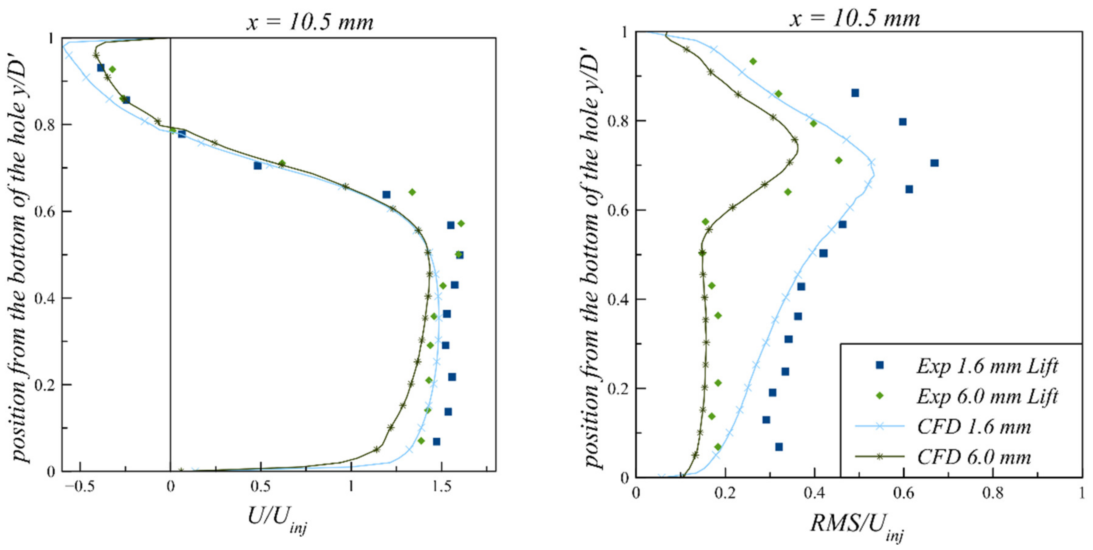
The CFD predictions of mean velocity and RMS velocity were compared with the experimental predictions in Figure 4 for both low and full lifts at x = 10.5 mm from the nozzle entrance, where the flow is the most complex, with steep mean velocity gradients and the presence of the full flow recirculation near the upper nozzle wall. Overall, the results show good agreement with the experimental data. Interestingly, by observing the experimental data of RMS velocity, noticeable differences can be observed when comparing the RMS velocity at low and full lifts, suggesting higher velocity fluctuations at the lower needle lift. This trend, as explained by experimentalists [8], is expected at the lower needle lift, due to the increased bottleneck effect at the needle seat. Hence, the liquid needs to squeeze through a smaller area and, therefore, is locally accelerated, with a higher mean velocity gradient that increases the turbulence level from this point onwards into the sac volume and the nozzle holes. The comparisons at the axial locations of x = 9.5, 13.5, and 16.5 mm—not presented here—showed similar agreement, and even better at locations further downstream, along with higher RMS predictions at all locations for the lower lifts. The comparisons between the predictions and the experimental results have been presented comprehensively in our previous works [13,25]; readers are hence advised to refer to those works for more details.
5.2. Flow Field Analysis
As mentioned above, experimental studies have recorded the occurrence of vortices in the injector volume, which are mainly of two types: one is a “hole-to-hole” connecting vortex, and the second type consists of double “counter-rotating” vortices emerging from the needle wall and entering the injector hole facing it. These vortices are considered prerequisites for the formation of vortex-type cavitation within the sac volume and nozzle holes (some examples of experimental observations are shown later in this section). In this study, possible mechanisms of formation of these vortices are discussed, and differences in the flow fields at low and full needle lifts are examined. The results of this study will lead to a better understanding of flow at different needle positions of the fuel injector, as they will help design engineers to produce improvements in the design of fuel injectors.
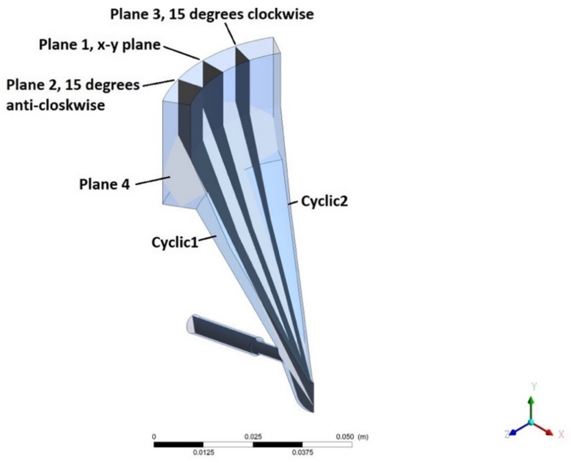
To analyse the flow field, we created planes in the injector geometry for predictions of both lift cases, as shown in Figure 5. The first plane, or plane 1 (P1), lies on the x–y plane at 0 degrees; i.e., the predicted plane goes through the axis of the nozzle hole. The second plane (P2) is 15 degrees anticlockwise, and the third plane (P3) is 15 degrees clockwise; i.e., two symmetrical planes on either side of the nozzle hole. Plane 4 (P4) is the predicted plane between the needle and the injector walls, as indicated in Figure 5. Cyclic1 and cyclic2 are the rotational periodic (cyclic) interface planes between the two adjacent symmetrical sections.
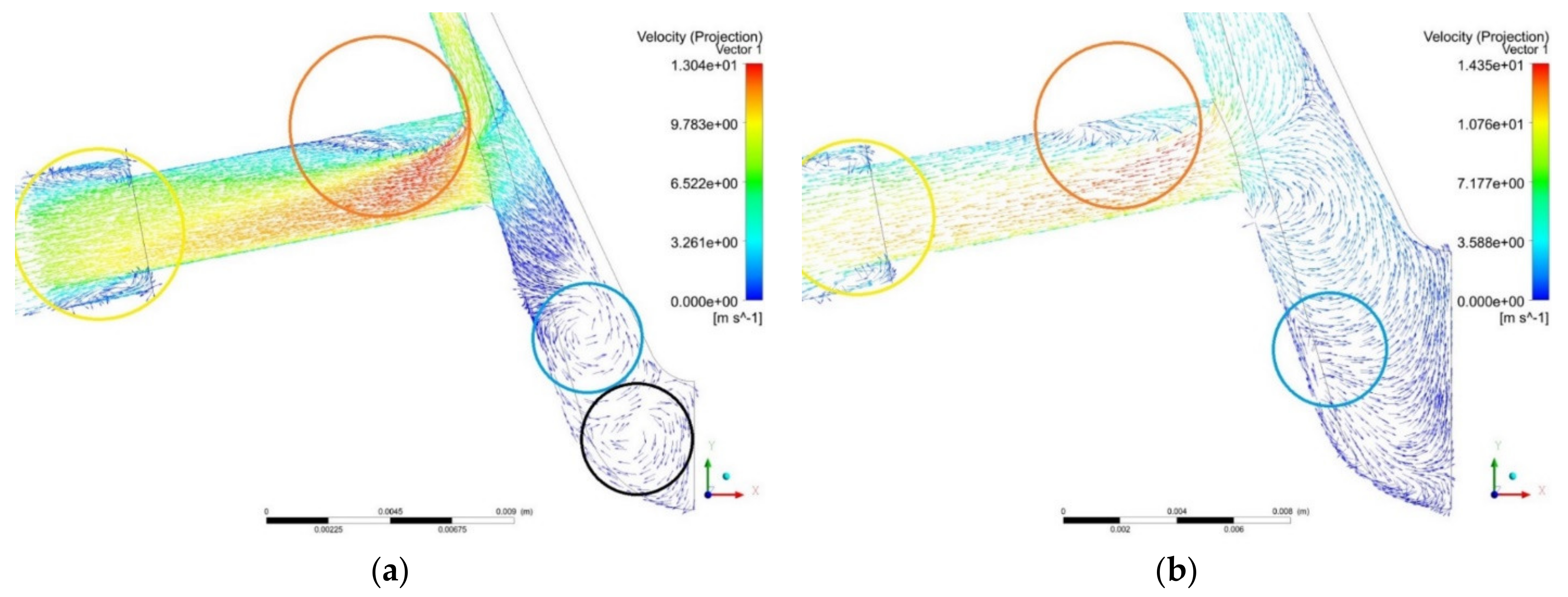
The velocity vectors on plane 1 in the sac region are compared in Figure 6a,b. The recirculation region due to fluid detachment at the upper entrance of the injector hole is highlighted by an orange circle in both panels. The vectors encircled in the yellow circle show fluid exiting the injector hole and entering the backflow hole, which has a step entrance that promotes the formation of the ring recirculation region at the injector hole exit. From the velocity vectors in the sac region, it can be seen that a large proportion of the liquid is drawn towards the injector hole due to lower local pressure in the injector hole. It is also evident that the incoming flow velocity vectors upstream of the nozzle hole between the needle and injector body are much higher with lower lift, due to its smaller flow passage downstream of the needle seat, which forces the fluid to accelerate; as mentioned before, this promotes the turbulence level with lower lift, which cascades downstream into the nozzle hole and the sac volume. On further observation of the sac region at lower and full needle lifts in Figure 6a,b, the development of vortices can be seen, as shown in the blue circle in the anticlockwise direction at low needle lift in Figure 6a, and in a clockwise direction at the full needle lift. In addition, there is another vortex near the bottom of the sac at the lower needle lift in Figure 6a, encircled in black, in a clockwise direction, which makes the flow in the sac volume more complex at the lower lift.
On observing the velocity vectors for the lower needle lift case on plane 2 (15 degrees anticlockwise from plane 1) in Figure 7a, it can be seen that a large proportion of liquid is drawn towards the injector hole, while the remainder goes into the sac volume. However, the lower pressure in the injector hole creates a negative pressure gradient and influences the flow field in the sac volume. Hence, fluid is further drawn towards the injector hole from the sac volume. In this process, the proportion of fluid that fails to enter the injector hole, impacting on the injector wall below the nozzle hole, is marked by a red circle. This leads to the development of a hole-to-hole connecting vortex; a similar phenomenon can be seen at full needle lift in Figure 7b. The majority of the fluid tends to enter the injector hole, whilst the remainder enters the sac volume. The part of the liquid that fails to enter the injector hole collides with the nozzle wall below, forming a hole-to-hole connecting vortex, as marked by the red circle. Moreover, further away from the hole, additional vortices can be seen in the sac volume at both needle lifts, as marked by the blue circles in Figure 7a,b. Furthermore, near the bottom of the sac volume, there is another clockwise vortex at the lower lift, encircled in black, as shown in Figure 7a—the same as that mentioned above in Figure 6a.
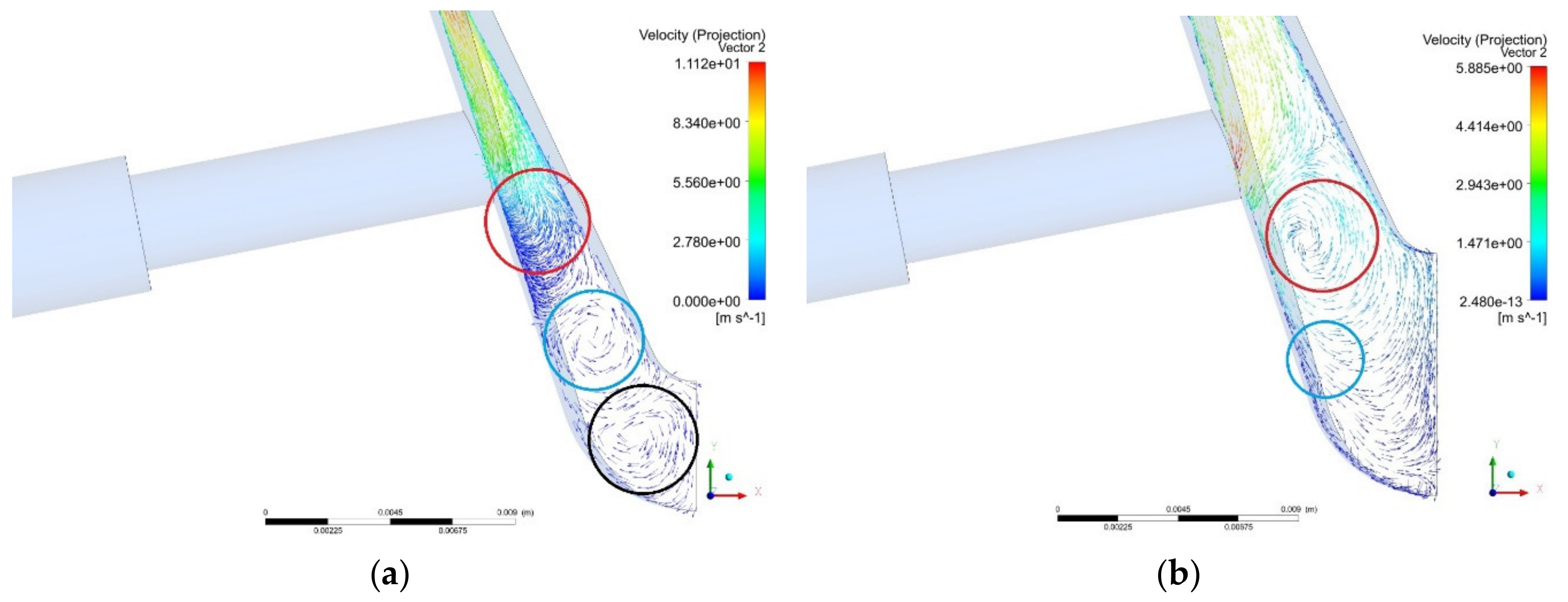
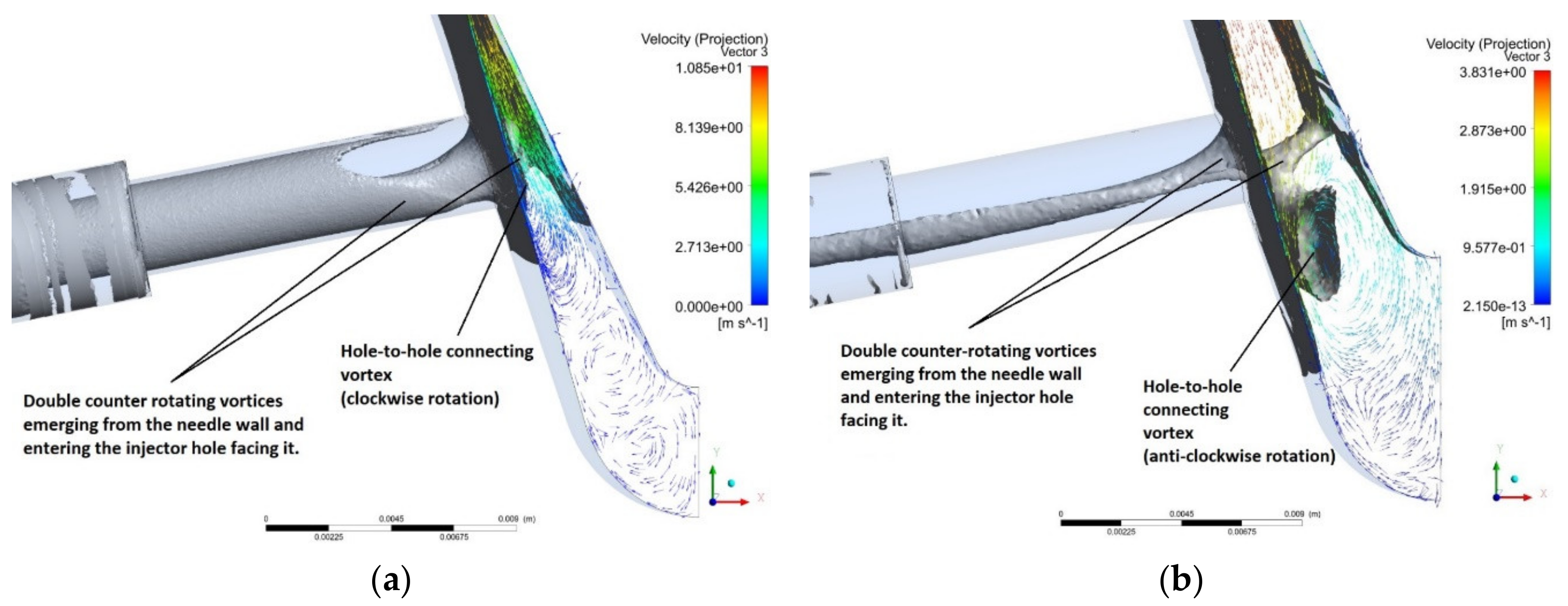
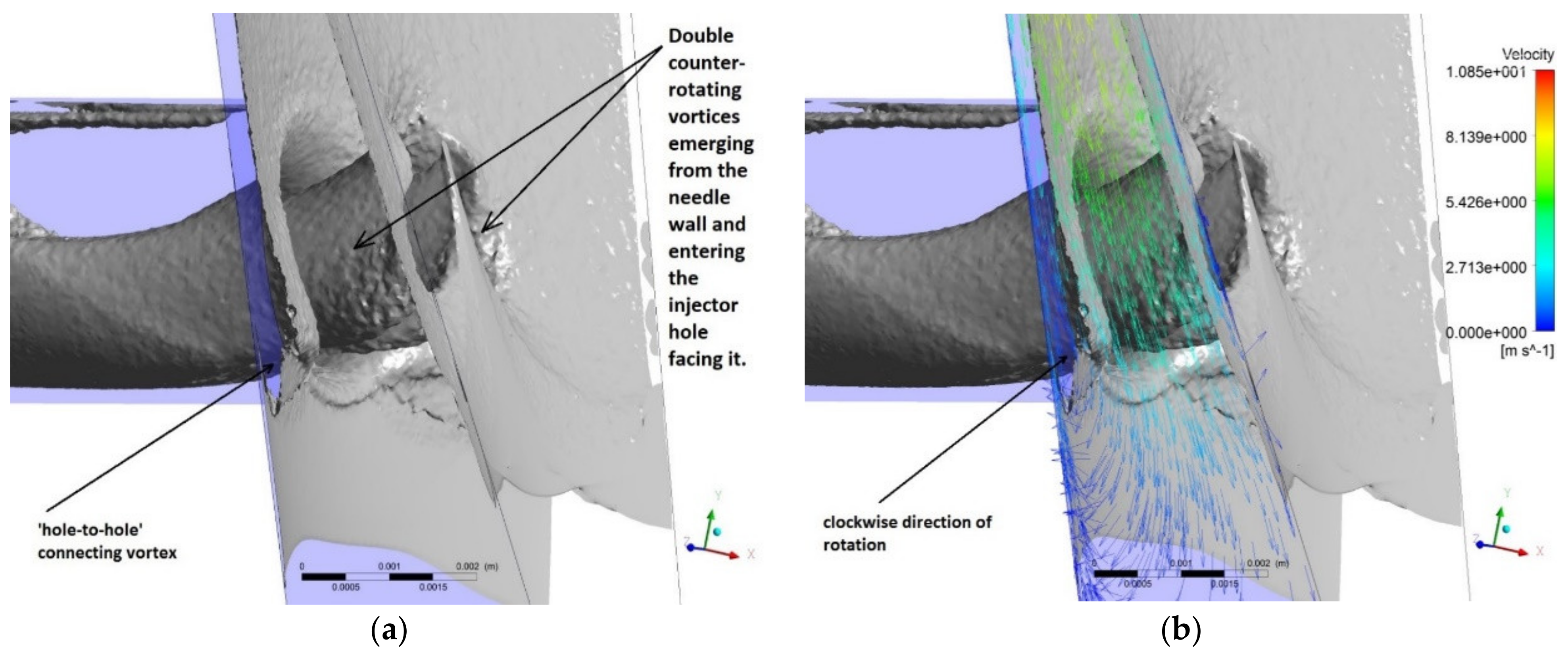
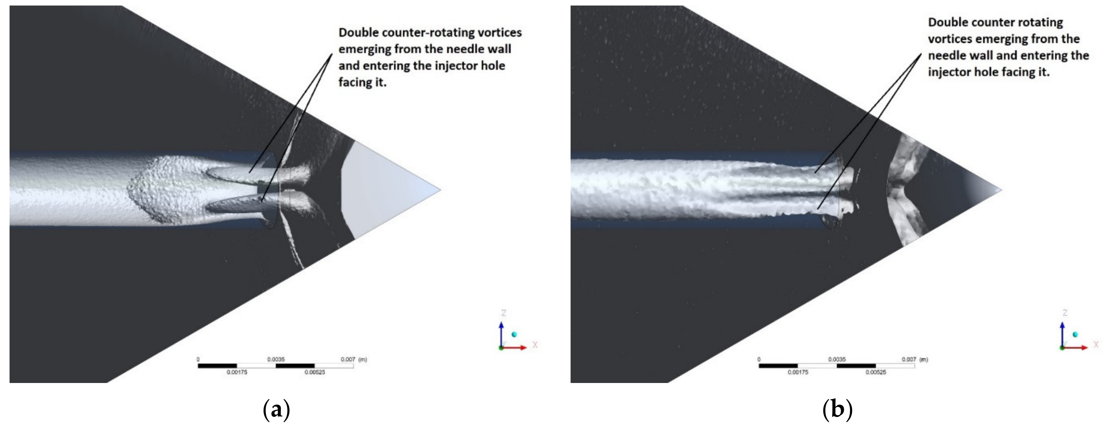
In Figure 8 and Figure 9, velocity vectors are plotted on the cyclic interface (cyclic1) at both needle lifts. The vectors at low needle lift in Figure 8a and Figure 9a clearly show hole-to-hole connecting vortices, along with additional vortices near the bottom of the sac volume, as discussed previously. In addition, the presence of a double counter-rotating vortex at the entrance of the nozzle and inside the nozzle is evident. To detect further vortices in the injector, the zoomed isosurface of vorticity (1% of the vorticity magnitude) was generated, as presented in Figure 10a,b for the low lift. These plots also clearly show the presence of “hole-to-hole” connecting vortices, as well as detecting the double “counter-rotating” vortices emerging from the needle wall and entering the opposing injector hole, as previously shown in Figure 8a and Figure 9a.
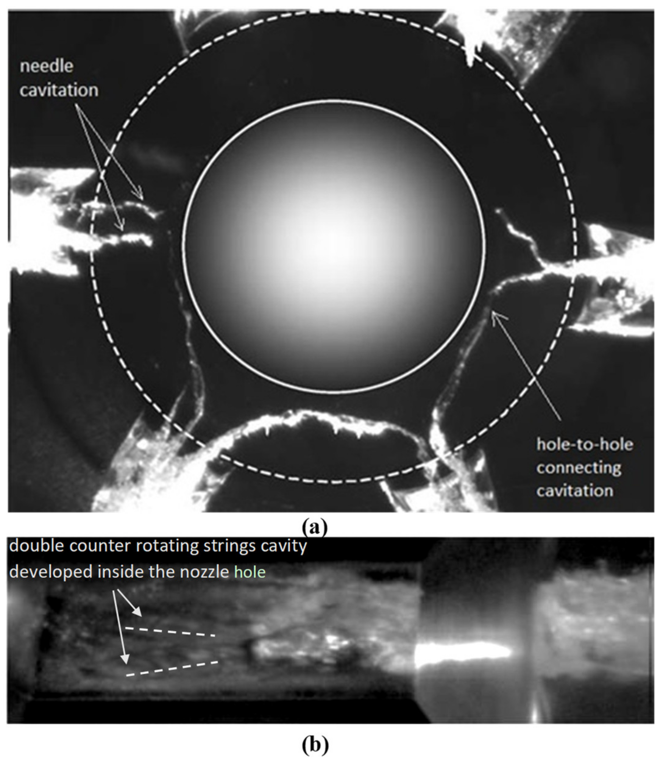
Similarly, at full needle lift in Figure 8b and Figure 9b, the velocity vectors on the cyclic interface (cyclic1) show a hole-to-hole connecting vortex. Similar isosurface of vorticity plots to those of the low needle lift case were also generated for the full needle case, as plotted in Figure 8b and Figure 9b. Again, the results clearly detect hole-to-hole connecting vortex, along with double vortices emerging at the needle surface and entering the injector holes facing it. It should also be noted that the predicted double “counter-rotating” vortices tend to merge into one another and disintegrate as they move further into the nozzle hole, as can be seen in Figure 8b and Figure 9b at full needle lift. The aforementioned vortices are in accordance with the experimental observations presented in Figure 11a,b.
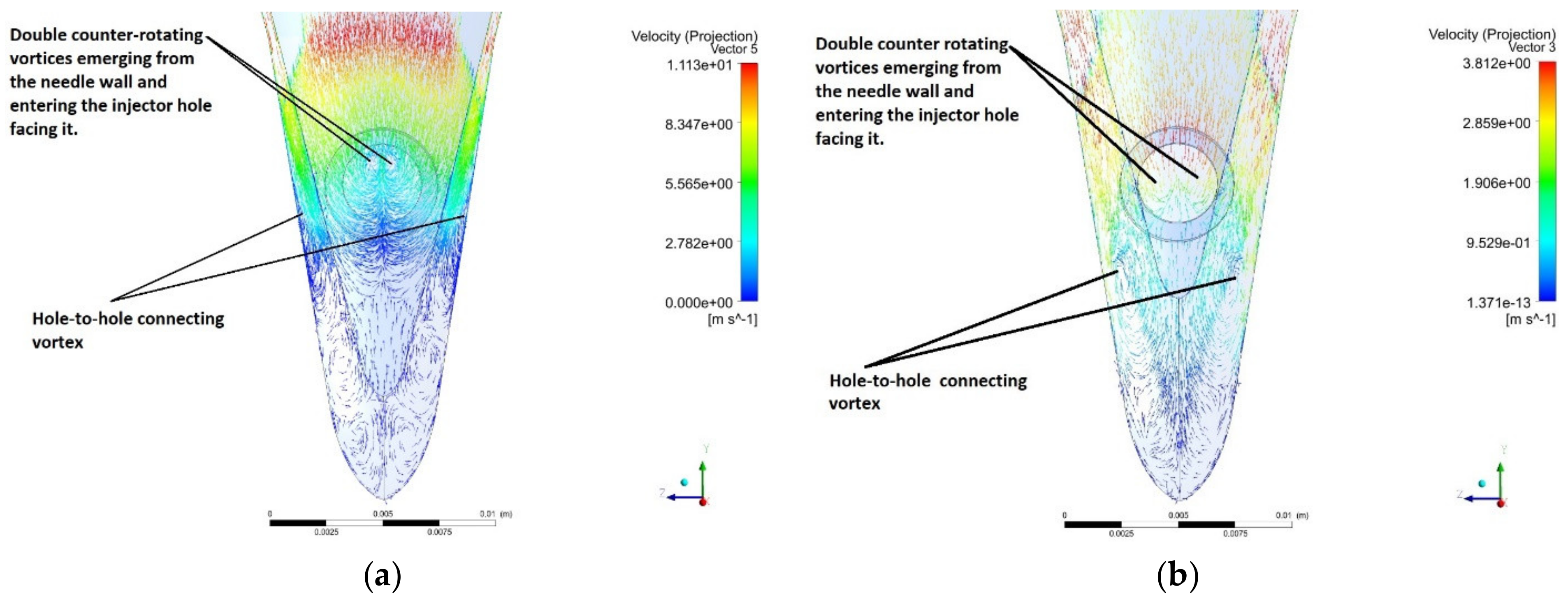
To further analyse the flow field, velocity vectors were plotted on plane 4 and the cyclic interfaces of cyclic1 and cyclic2 in Figure 12a,b at both needle lifts, along with the bottom isosurface of vorticity views of the injector, as shown in Figure 13a,b for low and full lifts, respectively. The velocity vectors in Figure 12a,b, along with the vorticity isosurfaces in Figure 13a,b, clearly show the prediction of double vortices emerging at the needle wall and entering the injector hole. Moreover, the velocity vectors on the cyclic interfaces in Figure 12a,b also indicate the prediction of hole-to-hole connecting vortices at both needle lifts. The predicted “hole-to-hole” vortices and double “counter-rotating” vortices emerging from the needle wall and entering the injector hole facing it are comparable to those detected in experimental studies of bottom-view [7] and nozzle hole [11] images of vortex cavities, as presented in Figure 11a,b.
5.3. Discussion
These vortices in multi-hole injectors—particularly in the present geometry—are mainly formed due to the geometry of the injector. The injector’s cavity, or the hollow volume where liquid flows, is shaped like a hollow section of two cones stacked on one another, with some specified clearance (as seen in Figure 3a and Figure 5) to accelerate the fluid in six symmetrically placed holes for the fluid to exit. As the liquid convects, the relatively lower local pressure at the injector holes attracts the most volume towards them and assists in its transport towards the exit. Nevertheless, not all of the fluid enters the injector holes; the proportion of liquid whose streamline does not lie on the injector hole path interacts with the surrounding wall below it, as well as with the fluid that already exists in the sac volume, thus forming vortices. At the same time, the relatively lower local pressure at the injector hole continues to attract fluid towards it, leading to the formation of hole-to-hole connecting vortices (as seen in Figure 8a,b, Figure 9a,b, Figure 10a,b and Figure 12a,b). However, some portion of the fluid penetrates and enters the sac volume further downstream, due to its higher momentum, but the already-present fluid in the injector sac volume causes resistance to more fluid entering the limited sac volume. The interaction between these flow streams leads to the formation of additional vortices in the sac volume (see Figure 6a, Figure 7a, Figure 8a, Figure 9a and Figure 12a), especially at the lower needle lift.
Now, regarding the double “counter-rotating” vortices that emerge from the needle wall and enter the injector hole facing it, as previously mentioned, due to the high momentum of the inflow above the needle seat, some proportion of the liquid enters the injector sac, but the higher local pressure in the sac resists the further entrance of liquid, due to the liquid already present within it. Thus, liquid at the proximity of the needle wall and injector hole begins to form counter-rotating vortices due to the symmetry in the nozzle geometry around this area; hence, the counter-rotation of vortices can also be the result of symmetry. As the local pressure at the injector hole is still relatively lower, it then draws further liquid towards the hole, leading to the formation of double counter-rotating vortices emerging from the needle wall and entering the injector hole facing it (see Figure 8a,b, Figure 9a,b, Figure 10a,b, Figure 12a,b and Figure 13a,b).
To identify differences between flow fields at the low and full needle lifts, velocity vectors are compared in Figure 6a,b, Figure 7a,b, Figure 8a,b, Figure 9a,b and Figure 12a,b, while isosurfaces of vorticity are compared in Figure 8a,b, Figure 9a,b and Figure 13a,b. The velocity vectors in Figure 6a,b and Figure 7a,b indicate the differences in the direction of rotation of hole-to-hole vortices at the lower needle lift compared to the full needle lift. The “hole-to-hole” connecting vortices are predicted in an anticlockwise direction at the lower needle lift, while the same is predicted with a similar magnitude but in the clockwise direction at the full needle lift. This noticeable difference can be attributed to the narrower clearance between the injector wall and needle wall at the lower needle lift, facilitating higher local fluid acceleration. Hence, at the lower needle lift, the portion of the fluid that enters the sac volume has more momentum than at the higher needle lift and, therefore, penetrates deeper into the sac. However, the already-present fluid in the injector sac volume resists the fluid entering into the sac. The interaction of those two flow streams with one another—and also with the injector walls within the limited sac volume—causes the formation of two vortices: one clockwise vortex near the bottom of the sac (black circles in Figure 6a and Figure 7a), and one anticlockwise hole-to-hole vortex above the first one, which extends up to the nozzle hole (Figure 6a, Figure 7a, Figure 9a, Figure 10b and Figure 12a). At the full needle lift, clearance is greater than at the low needle lift; hence, the fluid does not accelerate locally as much as at the low needle lift. Therefore, the proportion of fluid that does not enter the injector hole interacts with the fluid inside the sac with less resistance, and follows the rounded wall of the injector to develop into a single clockwise vortex (Figure 7b, Figure 8b, Figure 9b and Figure 12b). Therefore, the hole-to-hole connecting vortex is predicted to be clockwise at the full needle lift.
Finally, good quantitative and qualitative agreement between the predicted and experimental results shows the usefulness of the RANS modelling approach for such applications; however, there are limitations to this approach, as these models are derived based on assumptions that can lead to uncertainties and, therefore, the models may not be able to reproduce the entire flow field accurately. They may be quite accurate at some locations, while less so at others. Hence, RANS models often need to be tuned for specific cases using model constants. An alternative approach to address such problems is to use LES. The LES resolve most of the eddies (ideally up to the Taylor microscale), and model the smaller eddies using subgrid-scale models [34]. However, LESs are not recommended for this study, due to their high computational cost, because they require a significantly finer mesh than RANS. Moreover, the accuracy of LES depends on the timestep size, which is required to be smaller than the timescale of the smallest resolved motion. Furthermore, LES must run for a substantially long flow time in order to obtain stable statistics of the flow being modelled, which also increases the computational requirements. The hybrid RANS approach DES (detached-eddy simulation) offers a good compromise between LES and RANS in terms of computational requirements and result details; in this approach, the unsteady RANS models are employed at the boundary layer, while the LES treatment is applied to the separated region. This approach has been developed for wall-bounded flows with high Reynolds numbers and is therefore recommended for future research on the present class of flows (internal flows in fuel injectors), which are wall-bounded and have high Reynolds numbers.
6. Conclusions
Single-phase simulations were performed in a vertical axis-symmetrical six-hole diesel fuel injector, using the RANS approach with the realisable k-epsilon turbulence model. The main objective of this study was to gain insights into the flow fields related to the development of vortices, which decidedly influence the development of vortex cavitation. The following is a summary of the main findings and contributions of the present study:
The predictions were first assessed by comparing predicted mean and RMS velocities with experimental LDV data at both lower and nominally full needle lifts, which showed good agreement. The flow field analysis—in particular, the vortical structures—showed good similarities with the experimentally recorded high-speed images of the vortical cavitating structure in a multi-hole injector nozzle, confirming that these vortical structures are prerequisites of vortex cavitation in these injectors.
The simulated flow within the sac volume showed the presence of a complex, 3D, vortical flow structure. Two types of vortices were predicted: the first type was the “hole-to-hole” connecting vortices, while the second was double “counter-rotating” vortices emerging from the needle wall and entering the injector hole facing it.
The CFD predictions also indicate a difference in the flow pattern of the rotational direction of the “hole-to-hole” vortices between the low lift (anticlockwise) and the full needle lift (clockwise). This was argued to be due to their different flow passages between the injector wall and the needle, as explained in the Discussion section.
The predicated velocity vector results upstream of the nozzle hole between the needle and the injector walls showed that incoming flow velocities are much higher with lower lift, as expected, due to the smaller flow passage forcing the fluid to accelerate. This increases the turbulence level with the lower lift, which cascades downstream into the nozzle hole and the sac volume.
Good quantitative and qualitative agreement between the predicted and experimental results showed the usefulness of the RANS modelling approach for such applications. The limitations of RANS compared to LES models are discussed in Section 5.3, and it is recommended that the DES approach offers a good compromise between LES and RANS in terms of computational requirements and result details, making it ideal for wall-bounded flows at high Reynolds numbers, such as in the present application.
Author Contributions
A.K.: Methodology, Formal analysis, Writing—Original Draft, Writing—Review & Editing; A.G.: Conceptualization, Writing—Review & Editing, Supervision; J.N.: Writing—Review & Editing, Supervision, Funding acquisition. All authors have read and agreed to the published version of the manuscript.
Funding
City, University of London Award Studentship, CAS: E4G4BL7B00Z0H1.
Institutional Review Board Statement
Not applicable.
Informed Consent Statement
Not applicable.
Data Availability Statement
Not applicable.
Acknowledgments
The authors would like to thank City, University of London for the full scholarship and bursary for this research. The authors would also like to acknowledge the help provided by Chris Marshall via the use of the university cluster.
Conflicts of Interest
The authors declare that there is no conflict of interest.
Nomenclature
| = Cavitation number | Non-dimensional number |
| = Diameter of an injector hole | Mm |
| = Turbulent kinetic energy | m2s−2 |
| Number of injector holes | Non-dimensional number |
| = Pressure | Pa |
| = Mean pressure | Pa |
| Injection pressure | Pa |
| = Back (downstream) pressure | Pa |
| = Saturated vapour pressure | Pa |
| Volumetric flow rate | m3s−1 |
| = Reynolds number | Non-dimensional number |
| = Mean rate of strain tensor | s−1 |
| = Fluctuating rate of strain tensor | s−1 |
| = Temperature | K |
| = Velocity in the ith direction | ms−1 |
| = Mean velocity in the ith direction | ms−1 |
| = Fluctuating velocity component in the direction | ms−1 |
| Greek Symbols | |
| = Epsilon | m2s−3 |
| = Kronecker delta | Non-dimensional number |
| = Molecular viscosity of the fluid | Pa·s−1 |
| = Turbulent viscosity | Pa·s−1 |
| = Kinematic viscosity of the fluid | m2s−1 |
| = Kinematic viscosity of the liquid | m2s−1 |
| = Density | kg·m−3 |
| = Mean rate of rotation tensor | s−1 |
| = Angular velocity | rad·s−1 |
| Abbreviations | |
| CT | Computed tomography |
| CCD | Charge-coupled device |
| DES | Detached-eddy simulation |
| LDV | Laser Doppler velocimetry |
| LES | Large-eddy simulation |
| RANS | Reynolds-averaged Navier–Stokes |
| RMS | Root mean square |
Appendix A. Grid Independence Study at Low Lift
The mesh convergence study was performed by comparing the mean velocity and RMS velocity of the current grid with those of the subsequent grid of higher cell density at the low lift; the grids are presented in Table A1. The turbulence was simulated using the realisable k-epsilon model [24]. The near-wall turbulence was simulated using the EWT (enhanced wall treatment) method [33]. Steady-state simulations were performed, and were stopped at the convergence criteria of 1 × 10⁻⁴.

Table A1.
Grid used at low needle lift.
| Grid | Number of Cells | |
|---|---|---|
| 1 | 1,792,278 | 17.7 |
| 2 | 6,892,758 | 10.44 |
| 3 | 11,049,454 | 9.54 |
| 4 | 19,023,384 | 7.5 |
| 5 | 16,410,517 | 7.21 |
| 6 | 21,216,968 | 7.14 |
| 7 | 33,446,472 | 7.16 |
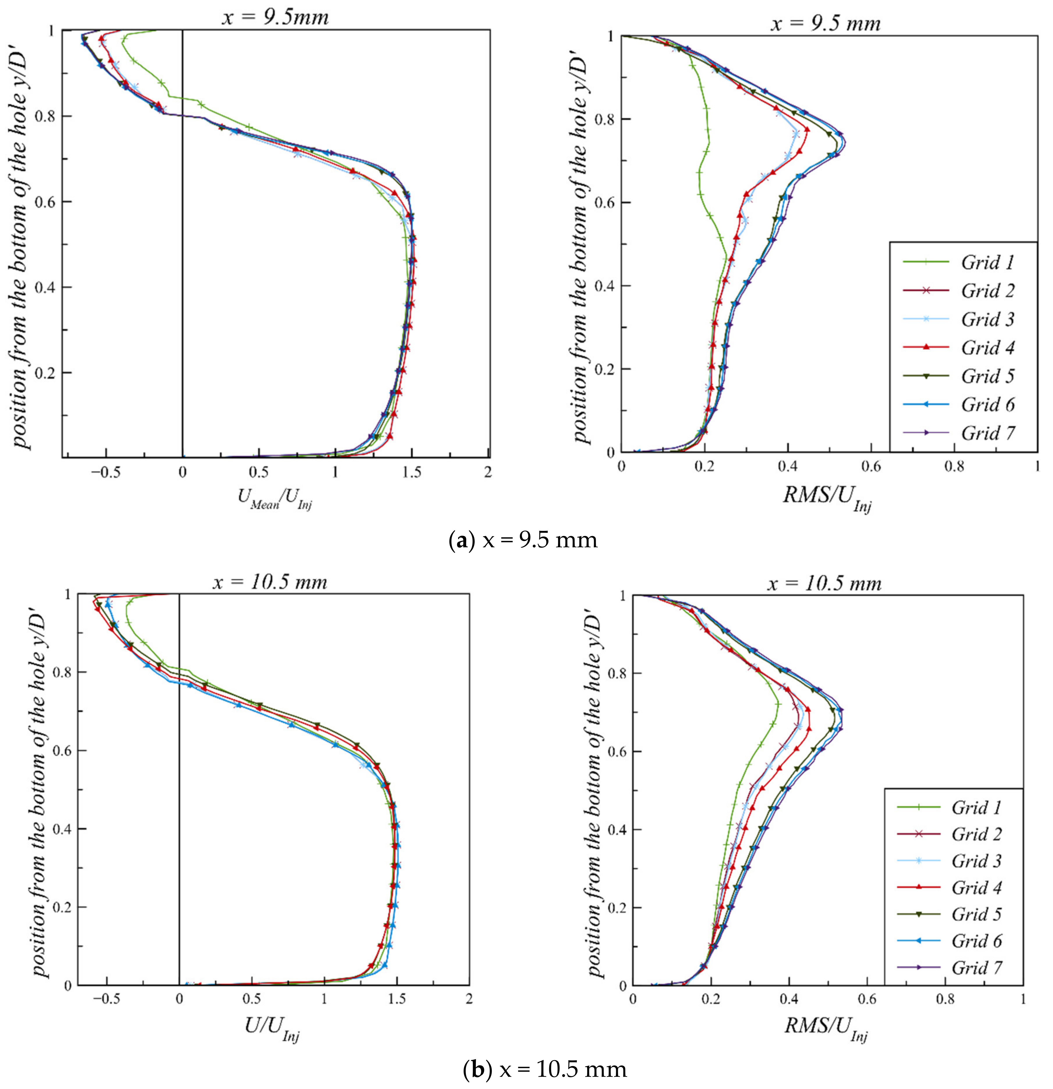
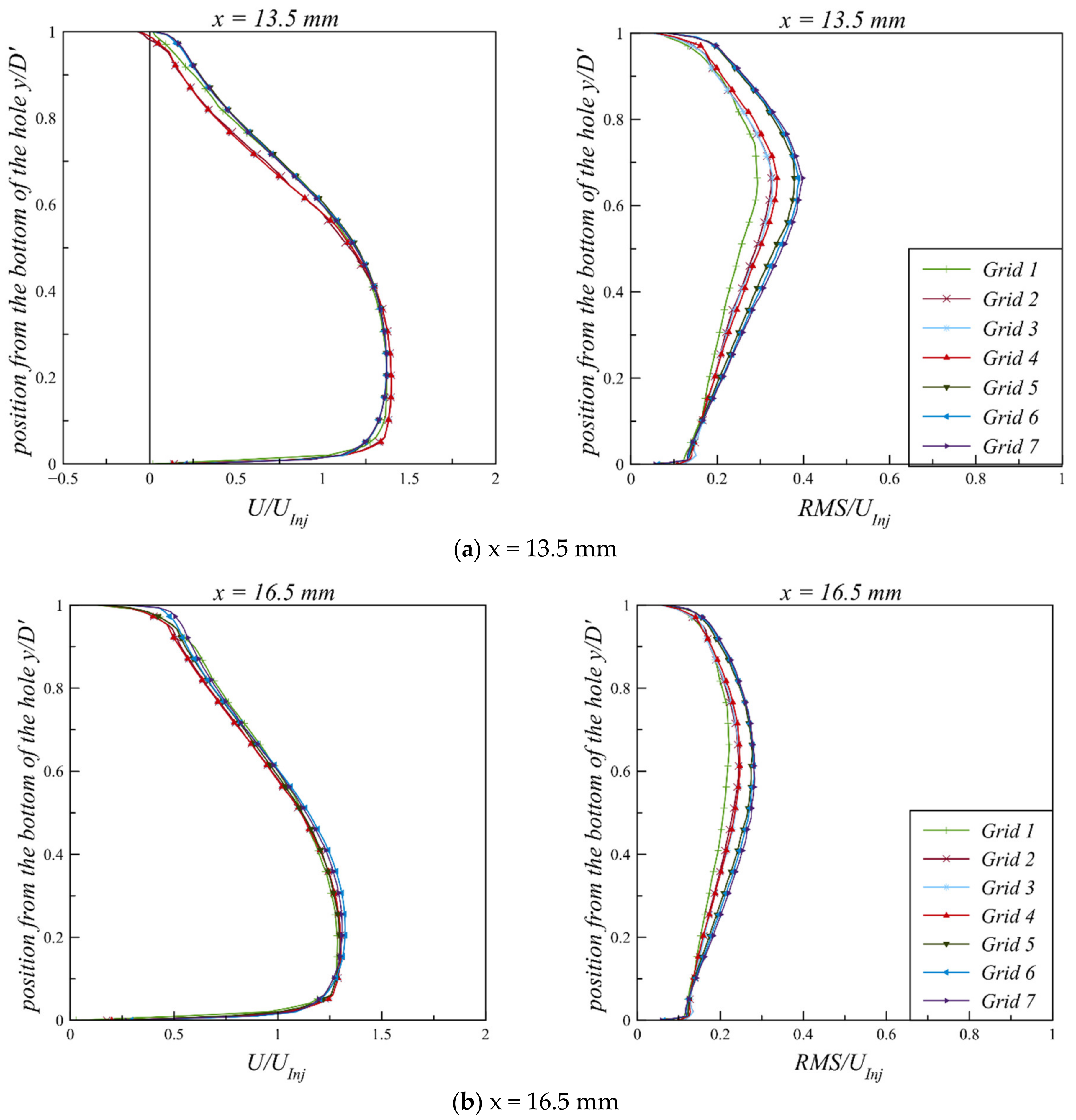
It can be seen from Figure A1 and Figure A2 that the velocity profiles begin to approach convergence with grids 6 and 7. The RMS velocity profiles in the same figures show an increase in RMS magnitude with the increase in mesh density in subsequent grids. This is because as the grid density increases, more accurate resolution in mean velocities across the finer grids can be achieved, resulting in a higher magnitude of mean velocity gradients. The RMS velocity is computed using the Boussinesq formulation [27], as shown in Equation (3); in this method, the RMS velocity magnitude depends directly on the mean velocity gradients. Therefore, as the mean velocity gradients increase, the RMS magnitude consequently increases. Here, from the RMS velocity magnitude results obtained using grids 6 and 7, it can be seen that grid independence is being approached; therefore, grid 6 was used for further assessment and analysis in the present study.
Figure A1.
Normalised mean axial velocity (left column) component and the corresponding RMS velocity (right column) of non-cavitating nozzle flow at CN = 0.44: (a) x = 9.5 mm and (b) x = 10.5 mm from the entrance.
Figure A1.
Normalised mean axial velocity (left column) component and the corresponding RMS velocity (right column) of non-cavitating nozzle flow at CN = 0.44: (a) x = 9.5 mm and (b) x = 10.5 mm from the entrance.

Figure A2.
Normalised mean axial velocity (left column) component and the corresponding RMS velocity (right column) of non-cavitating nozzle flow at CN = 0.44: (a) x = 13.5 mm and (b) x = 16.5 mm from the entrance.
Figure A2.
Normalised mean axial velocity (left column) component and the corresponding RMS velocity (right column) of non-cavitating nozzle flow at CN = 0.44: (a) x = 13.5 mm and (b) x = 16.5 mm from the entrance.

References
- Zhao, H. Advanced Direct Injection Combustion Engine Technologies and Development: Diesel Engines; Elsevier: Amsterdam, The Netherlands, 2009; Volume 2. [Google Scholar]
- Brennen, C.E. Cavitation and Bubble Dynamics; Cambridge University Press: Cambridge, UK, 2014. [Google Scholar]
- Soteriou, C.; Andrews, R.; Smith, M. Direct Injection Diesel Sprays and the Effect of Cavitation and Hydraulic Flip on Atomization. SAE Trans. 1995, 104, 128–153. [Google Scholar]
- Arcoumanis, C.; Gavaises, M.; Nouri, J.M.; Abdul-Wahab, E.; Horrocks, R.W. Analysis of the Flow in the Nozzle of a Vertical Multi-Hole Diesel Engine Injector. SAE Trans. 1998, 1245–1259. [Google Scholar] [CrossRef]
- Afzal, H.; Arcoumanis, C.; Gavaises, M.; Kampanis, N. Internal Flow in Diesel Injector Nozzles: Modelling and Experiments. IMechE Pap. S 1999, 492, 25–44. [Google Scholar]
- Arcoumanis, C.; Flora, H.; Gavaises, M.; Kampanis, N.; Horrocks, R. Investigation of Cavitation in a Vertical Multi-Hole Injector. SAE Trans. 1999, 108, 661–678. [Google Scholar]
- Arcoumanis, C.; Gavaises, M.; Nouri, J.M. The role of cavitation in automotive fuel injection systems. In Proceedings of the 8th International Symposium on Internal Combustion Diagnostics, Baden-Baden, Germany, 10–11 June 2008; pp. 159–167. [Google Scholar]
- Roth, H.; Gavaises, M.; Arcoumanis, C. Cavitation Initiation, Its Development and Link with Flow Turbulence in Diesel Injector Nozzles. SAE Trans. 2002, 111, 561–580. [Google Scholar]
- Mitroglou, N.; Nouri, J.M.; Gavaises, M.; Arcoumanis, C. Spray Characteristics of a Multi-Hole Injector for Direct-Injection Gasoline Engines. Int. J. Engine Res. 2006, 7, 255–270. [Google Scholar] [CrossRef] [Green Version]
- Mitroglou, N.; Gavaises, M.; Nouri, J.M.; Arcoumanis, C. Cavitation inside Enlarged and Real-Size Fully Transparent Injector Nozzles and Its Effect on near Nozzle Spray Formation. In Proceedings of the DIPSI Workshop 2011, Droplet Impact Phenomena & Spray Investigations, Bergamo, Italy, 27 May 2011; pp. 33–45. [Google Scholar]
- Mirshahi, M.; Nouri, J.M.; Yan, Y.; Gavaises, M. Link between In-Nozzle Cavitation and Jet Spray in a Gasoline Multi-Hole Injector. In Proceedings of the ILASS-Europe, 25th European Conference on Liquid Atomization and Spray Systems, Chania, Greece, 1–4 September 2013. [Google Scholar]
- Kumar, A.; Ghobadian, A.; Nouri, J.M. Assessment of Cavitation Models for Compressible Flows Inside a Nozzle. Fluids 2020, 5, 134. [Google Scholar] [CrossRef]
- Kumar, A.; Ghobadian, A.; Nouri, J. Numerical Simulation and Experimental Validation of Cavitating Flow in a Multi-Hole Diesel Fuel Injector. Int. J. Engine Res. 2021. [Google Scholar] [CrossRef]
- Giannadakis, E.; Gavaises, M.; Roth, H.; Arcoumanis, C. Cavitation Modelling in Single-Hole Diesel Injector Based on Eulerian-Lagrangian Approach. In Proceedings of the THIESEL International Conference on Thermo-and Fluid Dynamic Processes in Diesel Engines, Valencia, Spain, 7–10 September 2004. [Google Scholar]
- Giannadakis, E.; Gavaises, M.; Arcoumanis, C. Modelling of Cavitation in Diesel Injector Nozzles. J. Fluid Mech. 2008, 616, 153–193. [Google Scholar] [CrossRef] [Green Version]
- Papoutsakis, A.; Theodorakakos, A.; Giannadakis, E.; Papoulias, D.; Gavaises, M. LES Predictions of the Vortical Flow Structures in Diesel Injector Nozzles. SAE Tech. Pap. 2009. [Google Scholar] [CrossRef]
- Sou, A.; Biçer, B.; Tomiyama, A. Numerical Simulation of Incipient Cavitation Flow in a Nozzle of Fuel Injector. Comput. Fluids 2014, 103, 42–48. [Google Scholar] [CrossRef]
- Koukouvinis, P.; Naseri, H.; Gavaises, M. Performance of Turbulence and Cavitation Models in Prediction of Incipient and Developed Cavitation. Int. J. Engine Res. 2017, 18, 333–350. [Google Scholar] [CrossRef]
- Karathanassis, I.K.; Hwang, J.; Koukouvinis, P.; Pickett, L.; Gavaises, M. Combined visualisation of cavitation and vortical structures in a real-size optical diesel injector. Exp. Fluids 2021, 62. [Google Scholar] [CrossRef]
- Kolovos, K.; Kyriazis, N.; Koukouvinis, P.; Vidal, A.; Gavaises, G.; McDavid, R.M. Simulation of transient effects in a fuel injector nozzle using real-fluid thermodynamic closure. Appl. Energy Combust. Sci. 2021, 7, 100037. [Google Scholar] [CrossRef]
- Mamaikin, D.; Knorsch, T.; Rogler, P.; Wang, J.; Wensing, M. The effect of transient needle lift on the internal flow and near-nozzle spray characteristics for modern GDI systems investigated by high-speed X-ray imaging. Int. J. Engine Res. 2021. [Google Scholar] [CrossRef]
- Strotos, G.; Koukouvinis, P.; Theodorakakos, A.; Gavaises, M.; Bergeles, G. Transient heating effects in high pressure Diesel injector nozzles. Int. J. Heat Fluid Flow 2015, 51, 257–267. [Google Scholar] [CrossRef] [Green Version]
- Wilcox, D.C. Turbulence Modeling for CFD; DCW Industries: La Cañada Flintridge, CA, USA, 1998; Volume 2, ISBN 0963605151. [Google Scholar]
- Shih, T.-H.; Liou, W.W.; Shabbir, A.; Yang, Z.; Zhu, J. A New K-Epsilon Eddy Viscosity Model for High Reynolds Number Turbulent Flows: Model Development and Validation. Comput. Fluids 1995, 24, 227–238. [Google Scholar] [CrossRef]
- Kumar, A. Investigation of In-Nozzle Flow Characteristics of Fuel Injectors of IC Engines. Ph.D. Thesis, City, University of London, London, UK, 2017. [Google Scholar] [CrossRef]
- Nouri, J.M.; Whitelaw, J.H.; Yianneskis, M. A Refractive-Index Matching Technique for Solid/Liquid Flows. Laser Anemometry Fluid Mech. 1988, 3, 335. [Google Scholar]
- Versteeg, H.K.; Malalasekera, W. An Introduction to Computational Fluid Dynamics: The Finite Volume Method; Pearson Education: London, UK, 2007. [Google Scholar]
- Alfonsi, G. Reynolds-Averaged Navier–Stokes Equations for Turbulence Modeling. Appl. Mech. Rev. 2009, 62. [Google Scholar] [CrossRef]
- Schumann, U. Realizability of Reynolds—Stress Turbulence Models. Phys. Fluids 1977, 20, 721–725. [Google Scholar] [CrossRef]
- Lumley, J.L. Computational modeling of turbulent flows. In Advances in Applied Mechanics; Elsevier: Amsterdam, The Netherlands, 1979; Volume 18, pp. 123–176. ISBN 0065-2156. [Google Scholar]
- Fluent, A. 14.5 Theory Guide; ANSYS Inc.: Canonsburg, PA, USA, 2012. [Google Scholar]
- Patankar, S.V. Numerical Heat Transfer and Fluid Flow; CRC Press: Boca Raton, FL, USA, 1980; ISBN 9781315275130. [Google Scholar]
- Kader, B.A. Temperature and Concentration Profiles in Fully Turbulent Boundary Layers. Int. J. Heat Mass Transf. 1981, 24, 1541–1544. [Google Scholar] [CrossRef]
- Hanjalic, K. Will RANS survive LES? A View of Perspectives. J. Fluids Eng. 2005, 127, 831–839. [Google Scholar] [CrossRef]
Figure 1.
Representation of the simulated 3D model geometry of the injector and the needle/injector assembly at different needle lifts.
Figure 1.
Representation of the simulated 3D model geometry of the injector and the needle/injector assembly at different needle lifts.

Figure 2.
(a) Sketch of the needle and injector assembly, and the positions where the predictions of mean and RMS velocity were made; (b) recorded locations in the experimental data [8].
Figure 2.
(a) Sketch of the needle and injector assembly, and the positions where the predictions of mean and RMS velocity were made; (b) recorded locations in the experimental data [8].

Figure 3.
(a) One-sixth of the flow domain at the full needle lift, with periodic (cyclic) boundary conditions (the numbers represent the boundaries of flow domains: (1) inlet flow, (2) outlet flow, (3) injector and needle walls, and (4) periodic (cyclic) interface); (b) mesh of the flow domain; (c) axial plane mesh of the nozzle and sac volume flow domain.

Figure 4.
Normalised mean axial velocity (left column) component and the corresponding RMS velocity (right column) of non-cavitating nozzle flow at low lift (1.6 mm) CN = 0.44 and full lift (6.0 mm) CN = 0.45, and at x = 10.5 mm from the nozzle entrance; experimental data from [8].
Figure 4.
Normalised mean axial velocity (left column) component and the corresponding RMS velocity (right column) of non-cavitating nozzle flow at low lift (1.6 mm) CN = 0.44 and full lift (6.0 mm) CN = 0.45, and at x = 10.5 mm from the nozzle entrance; experimental data from [8].

Figure 5.
Planes and surfaces in the flow domain for flow-field analysis.

Figure 6.
Distribution of velocity vectors on plane 1 for the (a) low lift and (b) full lift; the vortices are encircled.
Figure 6.
Distribution of velocity vectors on plane 1 for the (a) low lift and (b) full lift; the vortices are encircled.

Figure 7.
Distribution of velocity vectors on plane 2 for the (a) low lift and (b) full lift; the vortices are encircled.
Figure 7.
Distribution of velocity vectors on plane 2 for the (a) low lift and (b) full lift; the vortices are encircled.

Figure 8.
(a) Distribution of velocity vectors on cyclic interface 1 for the (a) low lift and (b) full lift; the 3D isosurface of vorticity (1% of the vorticity magnitude) is also plotted.
Figure 8.
(a) Distribution of velocity vectors on cyclic interface 1 for the (a) low lift and (b) full lift; the 3D isosurface of vorticity (1% of the vorticity magnitude) is also plotted.

Figure 9.
(a) Distribution of velocity vectors on cyclic interface 1 for the (a) low lift and (b) full lift; the 3D isosurface of vorticity (1% of the vorticity magnitude) is also plotted.
Figure 9.
(a) Distribution of velocity vectors on cyclic interface 1 for the (a) low lift and (b) full lift; the 3D isosurface of vorticity (1% of the vorticity magnitude) is also plotted.

Figure 10.
(a) Zoomed 3D isosurface of vorticity (1% of the vorticity magnitude) of the sac region at low needle lift, generated to detect the presence of vortices; (b) 2D vectors of velocity are also plotted on the cyclic interface, in order to further detect vortices.
Figure 10.
(a) Zoomed 3D isosurface of vorticity (1% of the vorticity magnitude) of the sac region at low needle lift, generated to detect the presence of vortices; (b) 2D vectors of velocity are also plotted on the cyclic interface, in order to further detect vortices.

Figure 11.
High-speed digital images of cavitation in the fuel injector: (a) from the bottom, showing ‘‘hole-to-hole’’ connecting string cavitation and vortex cavitation structures emerging from the needle wall [7]; (b) from the side of the nozzle hole, showing two “counter-rotating strings cavities” inside the nozzle at full lift [11].

Figure 12.
Distribution of velocity vectors on plane 4 and cyclic1 and -2 for the (a) low lift and (b) full lift.
Figure 12.
Distribution of velocity vectors on plane 4 and cyclic1 and -2 for the (a) low lift and (b) full lift.

Figure 13.
Isosurface of vorticity (1% of the vorticity magnitude) viewed from the bottom of the injector to show the formation of the double-rotating vortices emerging from the needle wall and entering the injector hole at the (a) lower needle lift and (b) full needle lift.
Figure 13.
Isosurface of vorticity (1% of the vorticity magnitude) viewed from the bottom of the injector to show the formation of the double-rotating vortices emerging from the needle wall and entering the injector hole at the (a) lower needle lift and (b) full needle lift.

Table 1.
Operating conditions.
| Case | Series | Needle Lift (mm) | (bar) | (bar) | (m/s) | Volumetric Flow Rate Qt (L/s) | Temperature (°C) | ||
|---|---|---|---|---|---|---|---|---|---|
| 1 | 1 | 1.6 (low) | 0.45 | 18,000 | 2.55 | 1.80 | 8.43 | 0.487 | 25 ± 0.5 |
| 2 | 1.6 (low) | 0.45 | 18,000 | 2.55 | 1.80 | 8.43 | 0.487 | 25 ± 0.5 | |
| 2 | 1 | 6.0 (full) | 0.44 | 21,000 | 1.80 | 1.27 | 9.84 | 0.568 | 25 ± 0.5 |
| 2 | 6.0 (full) | 0.44 | 21,000 | 1.80 | 1.27 | 9.84 | 0.568 | 25 ± 0.5 |
Table 2.
Boundary conditions.
| Case | Needle Lift | (1) * Inlet (Mass Flow Rate) | (2) * Outlet (Constant Pressure) | (3) * Walls | (4) * Interface (Rotational Periodic) |
|---|---|---|---|---|---|
| 1 | 1.6 mm (lower) | 0.0726 kg/s | 180,000 N/m2 | No-slip | 60 |
| 2 | 6.0 mm (full) | 0.0847 kg/s | 127,000 N/m2 | No-slip | 60 |
* The numbers represent the boundaries of the flow domain, as indicated in Figure 3a.
Publisher’s Note: MDPI stays neutral with regard to jurisdictional claims in published maps and institutional affiliations. |
© 2021 by the authors. Licensee MDPI, Basel, Switzerland. This article is an open access article distributed under the terms and conditions of the Creative Commons Attribution (CC BY) license (https://creativecommons.org/licenses/by/4.0/).
Share and Cite
MDPI and ACS Style
Kumar, A.; Nouri, J.; Ghobadian, A. Predictions of Vortex Flow in a Diesel Multi-Hole Injector Using the RANS Modelling Approach. Fluids 2021, 6, 421. https://0-doi-org.brum.beds.ac.uk/10.3390/fluids6120421
AMA Style
Kumar A, Nouri J, Ghobadian A. Predictions of Vortex Flow in a Diesel Multi-Hole Injector Using the RANS Modelling Approach. Fluids. 2021; 6(12):421. https://0-doi-org.brum.beds.ac.uk/10.3390/fluids6120421
Chicago/Turabian StyleKumar, Aishvarya, Jamshid Nouri, and Ali Ghobadian. 2021. "Predictions of Vortex Flow in a Diesel Multi-Hole Injector Using the RANS Modelling Approach" Fluids 6, no. 12: 421. https://0-doi-org.brum.beds.ac.uk/10.3390/fluids6120421