Numerical Simulation of Propagation and Run-Up of Long Waves in U-Shaped Bays

Abstract

Wave propagation and run-up in U-shaped channel bays are studied here in the framework of the quasi-1D Saint-Venant equations. Our approach is numerical, using the momentum conserving staggered-grid (MCS) scheme, as a consistent approximation of the Saint-Venant equations. We carried out simulations regarding wave focusing and run-ups in U-shaped bays. We obtained good agreement with the existing analytical results on several aspects: the moving shoreline, wave shoaling, and run-up heights. Our findings also confirm that the run-up height is significantly higher in the parabolic bay than on a plane beach. This assessment shows the merit of the MCS scheme in describing wave focusing and run-up in U-shaped bays. Moreover, the MCS scheme is also efficient because it is based on the quasi-1D Saint-Venant equations.

1. Introduction

Tsunamis are some of the devastating natural disasters that threaten the population in coastal areas. Most tsunamis occur due to underwater earthquakes, landslides, and occasionally volcanic eruptions [1]. In a disaster event, tsunami heights and effects show a high variability along the coast. As was the case with the Sulawesi tsunami on 28 September 2018, very high tsunami waves were observed at several locations along the bay, particularly at the head of the bay, near the city of Palu, and at Pantoloan [2]. Since the bathymetry of Palu Bay has a form resembling a bay with a parabolic cross-section, the high tsunami run-up in Palu city can be attributed to the shoaling phenomenon in the U-shaped bay. As is well known, wave propagation in long and narrow bays can result in significant amplification due to the wave focusing mechanism [3,4,5,6]. Furthermore, wave amplification will be greater if the effects of reflection and diffraction of the waves are small, as they are in relatively long and narrow bays.

Wave propagation and run-up in U-shaped bays is a two-dimensional problem. However, if the flow is assumed to be uniform along the cross-section of the channel, as happens in a long and narrow channel, the conservation of mass and the balance of momentum can be well represented in the quasi-one-dimensional form of the Saint-Venant equations. Furthermore, if the bay has a U-shaped cross-section, the Saint-Venant conservative equation becomes explicit, allowing the formulation of a consistent conservative numerical scheme, as conducted here. These long, narrow bays and canyons are common in nature. Two examples are the triangular Sognefjoren fjord in Norway [7] and Scripps Canyon in California, which has a quasi-parabolic cross-section [8]. Further, the bathymetry of Palu Bay also has a parabolic cross-section shape, as shown in Figure 1a.

In the literature, there is an extensive discussion relating to this quasi-1D Saint-Venant equations, which includes the study of tsunami wave shoaling and run-up in U-shaped bays. The run-up of long nonlinear waves in narrow basins of special geometries is analyzed in [3,9,10]. For wave dynamics in U-shaped bays of a certain shape, analytical solutions can be derived using the hodograph (Legendre) transformation [11,12] or using the generalized Carrier–Greenspan transform [13,14,15]. Different from the literature above, where the shoreline dynamics on U-shaped bays are obtained through the transformed equations, in this study, we get the same result through direct application of the numerical MCS scheme to the quasi-one-dimensional Saint-Venant equations expressed in physical variables. Furthermore, with the same scheme, we also get other results related to wave dynamics in U-shaped bays, including here shoaling and run-up, which are in good agreement with the analytical formula [16]. All these assessments show the merit of the proposed MCS-scheme. Having a validated numeric scheme allows us to use it for a variety of narrow bays (including non-ideal ones). Hence, the main contribution of this research is the development of a numerical MCS scheme suitable for simulation of tsunami wave shoaling and run-up in U-shaped bays.

The structure of this paper is as follows. In Section 1, we present the quasi-1D Saint Venant formulation. We also re-formulate the MCS scheme so that it holds for wave flow problems in U-shaped bays. In Section 2, validation of the MCS scheme is carried out using analytical solutions. Here, we simulate the propagation and run-up of a Gaussian hump. The shoreline dynamics obtained for various types of U-shaped bays show good agreement with the analytical results of Garayshin et al. [14]. In Section 3, the numerical simulation of monochromatic wave shoaling is compared with the shoaling formula of Didenkulova and Pelinovsky [16]. Finally, we also assess the maximum run-up height of solitary waves in a parabolic bay, which is shown to have good agreement with the analytical run-up formula. In the last section, we give the conclusion.

2. Saint-Venant Equations and the MCS Model

In this first section, we formulate the precise form of the U-shaped bays considered, along with the Saint-Venant equations that are used throughout this article. The bay with a plane beach is the subject of the first discussion. Assume that the bay’s longitudinal direction is toward the positive x-axis. Suppose the bay has a regular cross-section in the shape of a parabola ${\left|y\right|}^m$, with $m>0$, which we refer to as U-shaped. Furthermore, U-shaped bays with a constant slope denoted as ${\mathcal{B}}_m$ is explicitly given by

$${\mathcal{B}}_m:d(x,y)=\alpha x+c{\left|y\right|}^m.$$

(1)

In Equation (1), the positive parameter $\alpha$ represents the bay slope, whereas the positive parameter c relates with the bay width. Figure 1b depicts the three-dimensional sketch of the U-shaped bay ${\mathcal{B}}_m$, for fixed m. Figure 1c,d shows the sloping channel depth $d(x,0)=\alpha x$ and the U-shaped cross-section ${c\left|y\right|}^m$, respectively.

Under the assumption that the wave flow is uniform over the channel cross-section, the free-surface depends on the longitudinal variable-x only, i.e., as $\eta (x,t)$. Further, we denote the total water height in the bay along the x-axis as

$$h(x,t)=\eta (x,t)-d(x,0),$$

(2)

whereas the total water height at other places as $H(x,y,t)=max\{h(x,t)-c|y{|}^m,0\}$ (see Figure 1d).

Further, following Garayshin [17], the cross-sectional area of fluid in bay ${\mathcal{B}}_m$ can be computed as

$$S(x,t)={\int }_{-{(h(x,t)/c)}^{1/m}}^{{(h(x,t)/c)}^{1/m}}H(x,y,t)dy={\int }_{-{(h(x,t)/c)}^{1/m}}^{{(h(x,t)/c)}^{1/m}}h(x,t)-c{\left|y\right|}^{m}dy=\frac{2m}{m+1}{c}^{-1/m}h{(x,t)}^{\frac{m+1}{m}}.$$

(3)

Note that the cross-section in Equation (3) also applies to U-shaped bays of the form $d(x,y)=f\left(x\right)+{c\left|y\right|}^m$, for any function $f\left(x\right)$. The fact that for U-shaped bays the cross-sectional area depends solely on the water height $h(x,t)$ opens up opportunities for a simpler governing equation and its numerical implementation, as discussed below. Under the assumption that flow is uniform across the channel cross-section, the conservation of mass and momentum balance appears in the form of one-dimensional Saint-Venant equations written below

$$\begin{array}{ccc}& & \frac{\partial S}{\partial t}+\frac{\partial Q}{\partial x}=0,\hfill \end{array}$$

(4)

$$\begin{array}{ccc}& & \frac{\partial Q}{\partial t}+\frac{\partial }{\partial x}\left(\frac{Q^2}{S}\right)+gS\frac{\partial h}{\partial x}=-gS\frac{\partial }{\partial x}d(x,0).\hfill \end{array}$$

(5)

In the above formulations, bottom friction is neglected, and the right-hand side term in (5) represents the body force.

The Saint-Venant Equations (4) and (5) are expressed in variables $S(x,t)$ and $Q(x,t)$, representing the cross-sectional area and the horizontal momentum, respectively. Moreover, the cross-section $S(x,t)$ depends solely on $h(x,t)$ via (3), whereas the momentum is $Q\equiv Su$, with $u(x,t)$ the horizontal velocity of fluid particles. Further, the Saint-Venant Equations (4) and (5) can be re-written as

$$\begin{array}{ccc}& & \frac{\partial S}{\partial t}+\frac{\partial Q}{\partial x}=0,\hfill \end{array}$$

(6)

$$\begin{array}{ccc}& & \frac{\partial u}{\partial t}+u\frac{\partial u}{\partial x}+g\frac{\partial \eta }{\partial x}=0.\hfill \end{array}$$

(7)

In deriving (7) from (4) and (5), we use the following relation

$$u{u}_x=\frac{1}{S}\left({\left(Qu\right)}_x-u{Q}_x\right).$$

(8)

We also simplify $gS(h_x+d_x(x,0))$ to $gS{\eta }_x$.

Numerical Methods

The numerical model used here is the conservative approximation of (6) and (7) applied on the staggered grid. The method is the generalization of the momentum conserving staggered-grid scheme, abbreviated as the MCS scheme (see [18]). We discussed a variant of this method which holds for a rectangular channel of varying depth and width in [19,20]. Since here we focus on channel with U-shaped cross-section, a short review of the MCS scheme for the quasi-1D of the Saint-Venant (6) and (7) is described below.

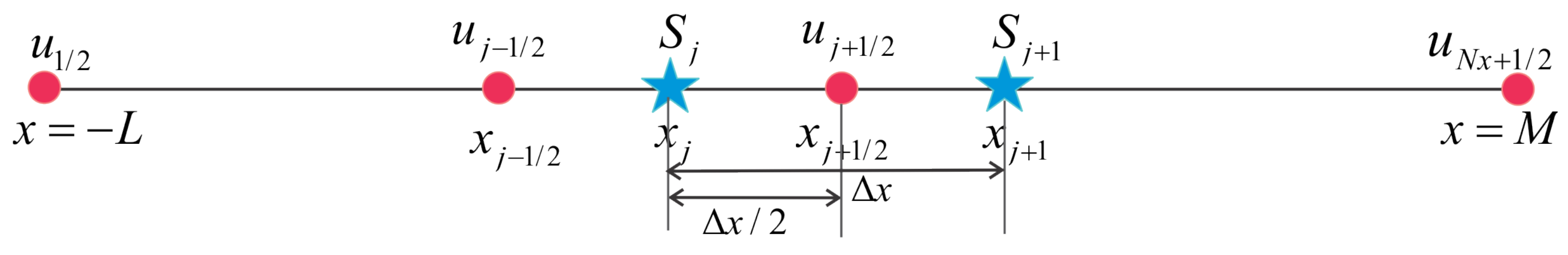
On the computational domain, e.g., $-L\le x\le M$, we apply a staggered grid partition, with the spatial grid size $\Delta x/2$, and the partition points

$$-L=x_{1/2},x_1,x_{3/2},\cdots ,x_{Nx},x_{Nx+1/2}=M.$$

As shown in Figure 2, two dependent variables S and u are calculated on different grid points: S is calculated on the full grid points, whereas u is calculated on the staggered grid points. At any discrete time $t_n$, we use notations $S(x_j,t_n)\equiv S_j^n$, for $j=1,\cdots ,Nx$, and $u(x_{j-1/2},t_n)\equiv u_{j-1/2}^n$, for $j=1,\cdots ,Nx+1$. The proposed discrete model of (6) and (7) is now

$$\begin{array}{ccc}& & {\displaystyle \frac{S_j^{n+1}-S_j^n}{\Delta t}}+{\displaystyle \frac{Q_{j+1/2}^n-Q_{j-1/2}^n}{\Delta x}}=0,\hfill \end{array}$$

(9)

$$\begin{array}{ccc}& & {\displaystyle \frac{u_{j+1/2}^{n+1}-u_{j+1/2}^n}{\Delta t}}+{\left(u{u}_x\right)}_{j+1/2}^n+g{\displaystyle \frac{{\eta }_{j+1}^{n+1}-{\eta }_j^{n+1}}{\Delta x}}=0.\hfill \end{array}$$

(10)

In (9), the momentum $Q_{j+1/2}$ is computed consistently using $Q_{j+1/2}{=}^{*}{S}_{j+1/2}{u}_{j+1/2}$, whereas ${}^{*}{S}_{j+1/2}$ is calculated using the upwind approximation

$${}^{*}{S}_{j+1/2}=\left\{\begin{array}{cc}{S}_j,\hfill & \hfill \mathrm{for}{u}_{j+1/2}\ge 0,\\ \hfill S_{j+1},& \hfill \mathrm{for}{u}_{j+1/2}<0.\end{array}\right.$$

(11)

Adopting the relation (8), a consistent approximation for the advection term reads

$$u{u}_x{|}_{j+1/2}={\displaystyle \frac{1}{{\overline{S}}_{j+1/2}}}\left({\displaystyle \frac{{\overline{Q}}_{j+1}{}^{*}{u}_{j+1}-{\overline{Q}}_j{}^{*}{u}_j}{\Delta x}}-u_{j+1/2}{\displaystyle \frac{{\overline{Q}}_{j+1}-{\overline{Q}}_j}{\Delta x}}\right),$$

(12)

whereas

$${\overline{S}}_{j+1/2}={\displaystyle \frac{S_j+S_{j+1}}{2}},{\overline{Q}}_j={\displaystyle \frac{Q_{j-1/2}+Q_{j+1/2}}{2}},$$

(13)

and the first-order upwind approximation for horizontal velocity is

$${}^{*}{u}_j=\left\{\begin{array}{cc}{u}_{j-1/2},\hfill & \mathrm{for}{\overline{Q}}_j\ge 0,\hfill \\ u_{j+1/2},\hfill & \mathrm{for}{\overline{Q}}_j<0.\hfill \end{array}\right.$$

(14)

As a resume, the MCS-scheme is (9) and (10), whereas, for each time step, we only need to compute $S_j^{n+1}$ and $u_{j+1/2}^{n+1}$. Once $S_j^{n+1}$ is obtained from (9), we can calculate $h_j^{n+1}$ from (3), and vice versa. Then, ${\eta }_j^{n+1}$ can be obtained from $h_j^{n+1}+d_j$, the discrete form of (2). Furthermore, the MCS-scheme (9) and (10) is explicit, and it is second-order accurate for the linear terms as well as first-order accurate for the nonlinear terms. These properties are directly inherited from the MCS-scheme for the one-dimensional SWE, as discussed in [18].

To conduct run-up simulations, the computations should incorporate both wet and dry areas. For this purpose, a simple wet–dry procedure should be adopted; i.e., the momentum calculation (10) is deactivated in the dry area. Here, a location is considered as dry if the water level is less than a prescribed threshold value $h_{thres}$, or equivalently if the area $S_j$ in (12) is less then $S_{thres}\equiv S\left(h_{thres}\right)$ from (3).

3. Propagation and Run-Up in Channel ${\mathcal{B}}_m$

In this section, we observe the capability of the MCS-scheme (9) and (10) in simulating wave propagation in the channel bed ${\mathcal{B}}_m$. Moreover, the accuracy of the scheme in computing the moving shoreline is shown via comparison with the analytical result of Garayshin et al. [14].

3.1. Simulation of an Initial Hump

Consider the channel bay ${\mathcal{B}}_m$, with parameters $m=3$ and $\alpha =0.02$, stretched over a domain $-4000$ m $\le x\le 100$ m. The acceleration of gravity is taken to be $g=9.81$ m/s${}^2$. Here, we choose the initial surface to be a hump given by

$$\eta (x,0)=0.03exp\left(-{\left(\frac{x+1500}{500}\right)}^2\right),$$

(15)

which is released with zero initial velocity. The initial surface (15) represents a positive hump with the peak amplitude $0.03$ m, located at $x=-1500$ m. The absorbing boundary condition is applied to the left boundary $x=-L$, i.e.,

$$u(-L,t)=-\sqrt{\frac{g}{h(-L,t)}}\eta (-L,t).$$

Since there is a sloping coast on the right, here we just take zero velocity for the right boundary $u(M,t)=0$. The computation is conducted using $\Delta x=0.1$ m and $\Delta t=0.05$ s.

The computational result is given in Figure 3a as the top view of the normalized surface $\eta (x,t)/a_0$. As shown in the figure, the initial hump splits into two waves that propagate in two opposite directions. One wave travels offshore, and the other wave travels towards the shore with increasing amplitude and decreasing wavelength. Then, the waves reflect from the shore, undergo a phase change, and propagate offshore with a decreasing amplitude. Figure 3b,c shows the enlarged contour plots of $\eta (x,t)/a_0$ and $u(x,t)/u_0$ near shoreline. Note that $u_0\equiv ma{x}_{t}u(x,t)$, whereas the red curves represent the boundary between the wet and dry areas. This result shows the capability of the MCS scheme in handling the wet–dry procedure, which here uses the threshold parameter $h_{thres}=1\times {10}^{-6}$ m. In this way, we can track the shoreline as a function of time. In the following discussion, this numerical shoreline is compared with the analytically computed shoreline of Garayshin et al. [14].

3.2. The Shoreline Dynamics

In this subsection, we take a closer look at the previous simulation and carefully observe the resulting shoreline dynamic. It is shown here that different shoreline dynamics occur when the channel has different cross-section types.

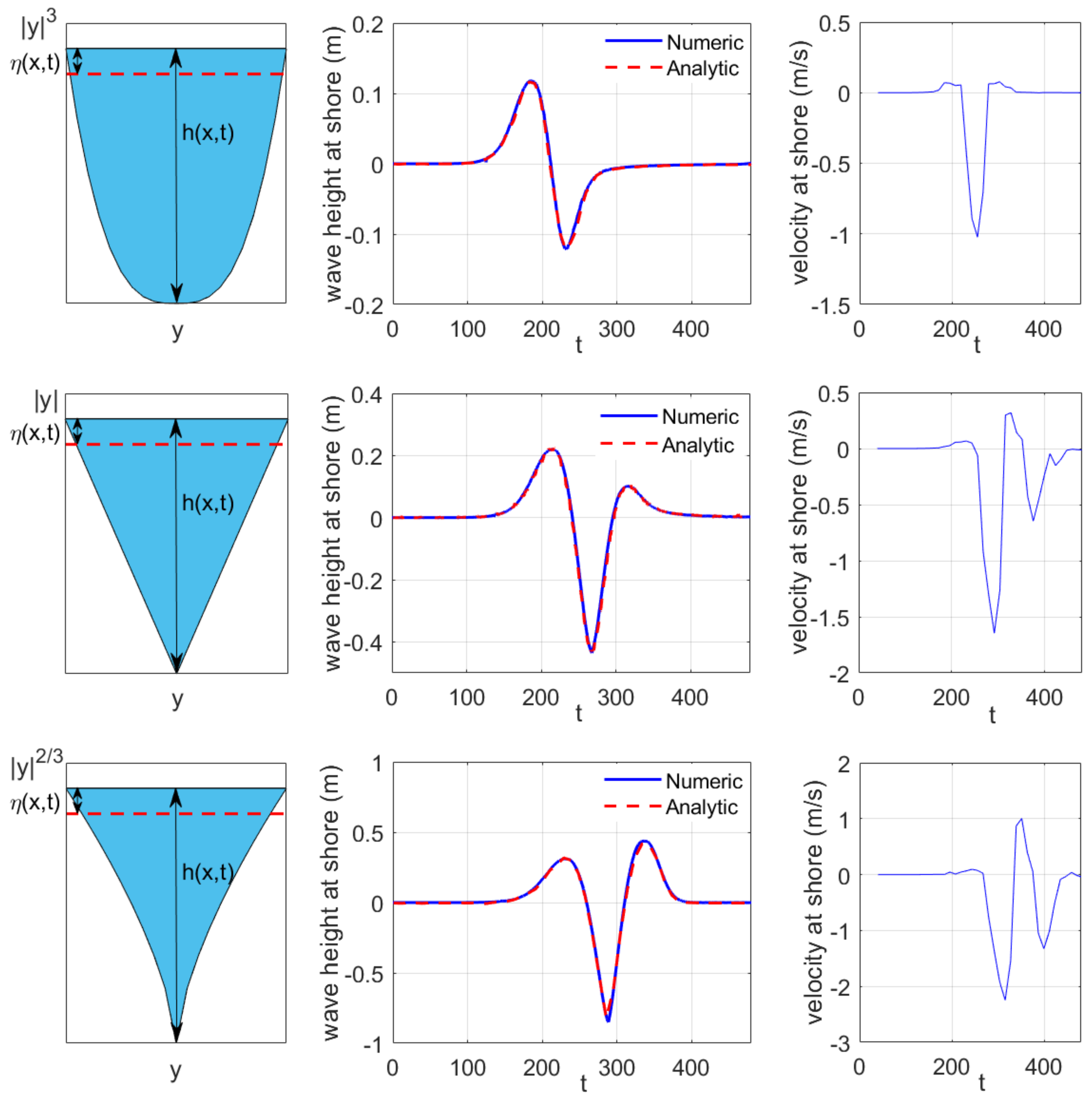
From the previous simulation, i.e., the wave simulation on channel ${\mathcal{B}}_m$, with $m=3$, the shoreline dynamics is clearly depicted in Figure 4 (top). As shown in the figure, the hump hits the shoreline and produces a positive run-up, which is followed by a negative run down. The figure also shows that the numerical shoreline can capture the analytical shoreline almost perfectly. Using the same set of parameters, other simulations using two different channels ${\mathcal{B}}_m$, with $m=1$ and $m=2/3$, were conducted. In both cases, the numerical shoreline show good agreement with the analytical shoreline [14] (see Figure 4, middle and bottom). This agreement more or less reveals the accuracy of the MCS-scheme proposed here, including its ability to simulate run-up waves in U-shaped bays.

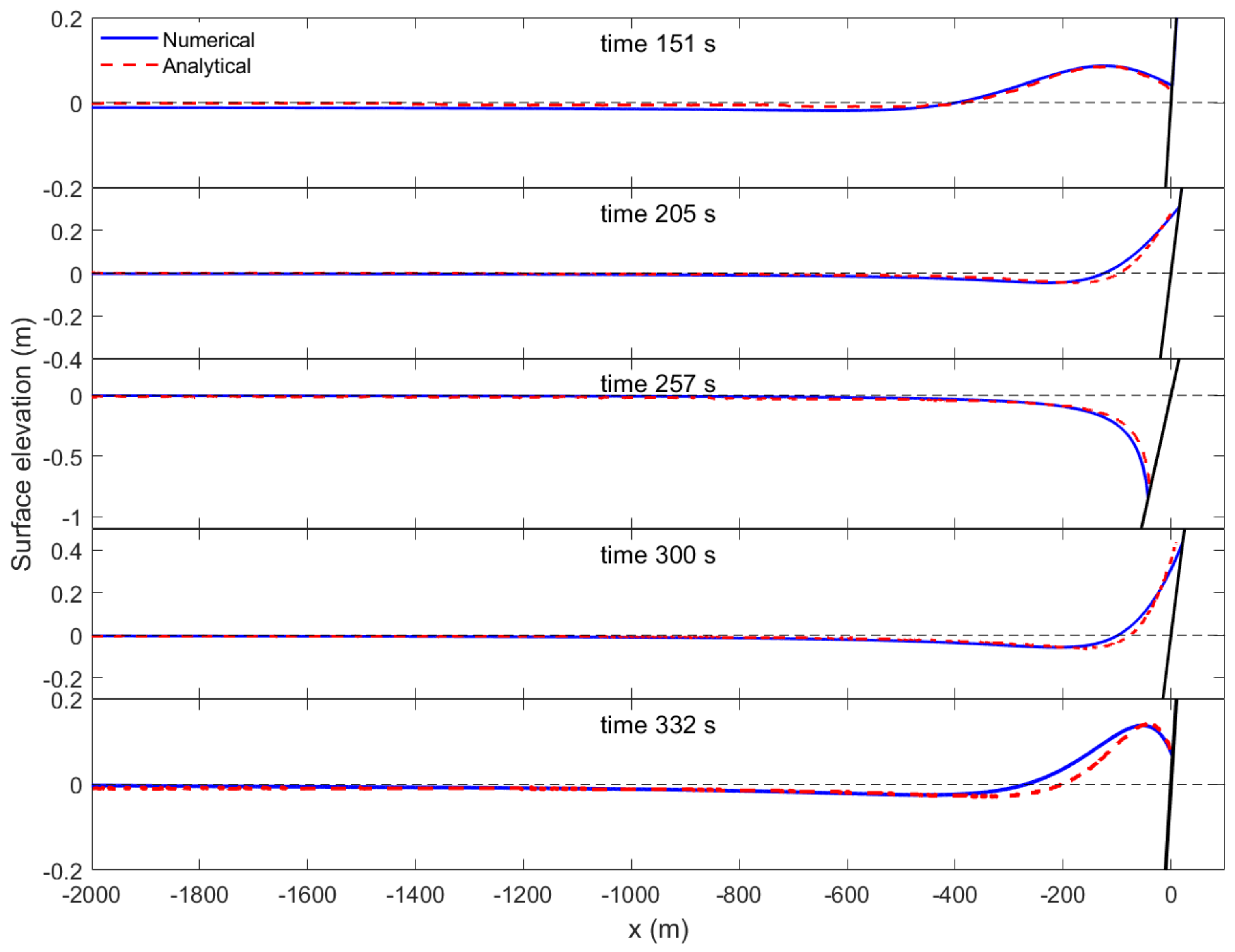
In a more detailed observation, the three different shorelines in Figure 4 show three different run-up phenomena, which depend solely on the channel type. In channel ${\mathcal{B}}_3$, the initial wave resulted in a positive run-up followed by a negative run-down, whereas, in channel ${\mathcal{B}}_1$, a positive run-up, followed by a negative run-down, and another positive run-up of lower amplitude are observed. In channel ${\mathcal{B}}_3$, the maximum run-up and minimum run-down reach roughly four times the amplitude of the incoming wave. A similar run-up phenomenon is also observed in channel ${\mathcal{B}}_{2/3}$. The initial hump hit the channel and make a positive run-up, a negative run-down, and a second positive run-up that is higher than the first. This detailed process of run-up and run-down described above is captured in the subsequent plots shown in Figure 5. The figure shows the nearshore wave dynamic from the numerical MCS-scheme in comparison with the analytical result of Garayshin et al. [14]. Good agreement is obtained in terms of both the surface plot ands the shoreline dynamics.

4. Propagation and Run-Up in Channel ${\mathcal{B}}_m^{*}$

In this section, we examine in detail another type of bay, namely a bay with a non-linear coastal slope, as suggested by the rigorous study of Didenkulova and Pelinovsky [16], with important results, one of them being that traveling waves do exist for bay bathymetry of the form

$${\mathcal{B}}_m^{*}:d^{*}(x,y)=\alpha x^{4m/(3m+2)}+c{\left|y\right|}^m.$$

(16)

When compared to (1), bay bathymetry (16) depends on x in a non-linear manner and is therefore not a plane beach. In Figure 6a, the curves of $x^{4m/(3m+2)}$, for varying m, are plotted. As shown in the figure, they are convex curves if $m>2$, linear curves if $m=2$, and concave curves if $m<2$. Figure 6b–e shows the corresponding 3D sketch of the channel-bays ${\mathcal{B}}_m^{*}$.

Didenkulova and Efim [16] calls this type of bathymetry a ‘non-reflecting bay’. In this type of bay, the traveling wave can propagate over a large distance without being reflected. An assessment of tsunami run-up in these bays is important because, based on the analytical study in [16], run-up heights in these bays are much greater than those on sloping beaches. In this section, we adopt ‘non-reflecting’ bays, ${\mathcal{B}}_m^{*}$, and conduct simulation related to two important phenomena: shoaling and run-up. We use a monochromatic wave influx for shoaling, while we use a solitary hump for the run-up. The two wave types used here were selected to fit the analytical formula of Didenkulova and Pelinovsky [16]. At the same time, simulation acts as a validation of the numerical MCS scheme.

4.1. Shoaling and Run Up of a Monochromatic Wave

For U-shaped bays with bathymetry given by (16), a monochromatic wave with amplitude A will undergo a shoaling process according to formula

$$A\sim d^{*}{(x,0)}^{-\left(\frac{1}{4}+\frac{1}{2m}\right)}\sim x^{-\frac{m+2}{3m+2}},$$

(17)

whereas the last relation is obtained after we use $d^{*}(x,0)\sim x^{4m/(3m+2)}$. As discussed in [16], this is an exact shoaling formula that holds for Saint-Venant Equations (6) and (7).

In this study, a simulation of a monochromatic wave propagating over the U-shaped bays ${\mathcal{B}}_m^{*}$ (16) is performed and the shoaling process is observed, to be confirmed by the analytical shoaling Formula (17). For this purpose, the same numerical MCS-scheme (9) and (10) can be used, because the bay bathymetry (16) has the same $S(x,t)$ cross-sectional area as in (3).

In the simulation, a computational domain $-L\le x\le M$ is taken, and the bathymetry (16), with a certain prescribed m, is adopted. For $m=2$, the bathymetry (16) is $d^{*}(x,0)=\alpha x$. A monochromatic wave with amplitude $a_0$ is imposed from the left boundary using

$$\eta (-L,t)=a_{0}sin\left(2\pi t\right).$$

(18)

All simulations on these ${\mathcal{B}}^{*}$ bays use a small-scale domain, with the gravitational acceleration normalized to one. To be precise, we adopt the following parameters: $L=1$ m, $M=0.2$ m, $\alpha =0.1$, and wave amplitude $a_0=0.002d_0$, with $d_0\equiv \left|d^{*}(-L,0)\right|$, which represents the maximum depth of the bay along the main axis. The first computation is conducted in a parabolic bay model, i.e., $m=2$, and we adopt parameters $\Delta x=5e-4$ m and $\Delta t=7e-4$ s. As time progresses, this monochromatic wave enters the U-shaped bay, where, as its depth decreases, the wave experiences a shoaling process (see Figure 7a). The result of a similar simulation, but for ${\mathcal{B}}_m^{*}$, with $m=3$, is given in Figure 7b. As shown in both figures, the numerical surface amplitude undergoes shoaling that follows exactly the analytical shoaling Formula (17). Good agreement is also shown in simulations with other m, but the results are not presented here because they show similar phenomena.

4.2. Run Up of a Solitary Hump

As discussed by Didenkulova and Pelinovsky [16], the U-shaped bay of (16) admits traveling wave solutions. In this type of bay, tsunami waves can travel over long distances without reflection and transfer all their energy to the shore, which can lead to extreme wave amplification on the coast.

In this section, we conduct numerical simulation using a long solitary wave hump over the U-shaped bay ${\mathcal{B}}_m^{*}$. This simulation is similar to the previous ones, except that here we use a wave influx of a solitary wave type.

Consider a U-shaped narrow bay ${\mathcal{B}}_m^{*}$ (16), which is stretched over $-L\le x\le M$, so the deepest part is $d_0=\left|d^{*}(-L,0)\right|=\alpha L$. Similar to the previous simulations, the solitary wave is imposed from the left boundary using

$$\eta (0,t)=a_0{sech}^2\left(\frac{2a_{0}g}{4d_0^2}t\right).$$

(19)

As analytically derived in [16], the approaching solitary wave in the U-shaped bay produces the maximum run-up height according to the formula

$$\frac{R_2}{a_0}=\frac{2}{3}\frac{\mu }{\alpha }{\left(\frac{a_0}{d_0}\right)}^{1/2},\mu =2\frac{3m+2}{m+2}\sqrt{\frac{m+1}{m}}.$$

(20)

With the parameters used in the simulations, i.e., $L=1$ m and $\alpha =0.1$, the maximum depth is $d_0=0.1$ m. Here, we adopt a solitary hump with amplitude $a_0=0.05d_0$. The small value for this amplitude is chosen to have a long wave that will propagate without breaking until the wave reaches the beach boundary. The computation is conducted using $\Delta x=5e-4$ m and $\Delta t=9e-4$ s, and the acceleration of gravity is normalized to one, with the threshold water depth $h_{thres}=1e-6$ m.

As time progresses, the wave enters the bay, and up onto the beach, where it is then reflected by the beach on the right. The simulated free surface plots at subsequent times are shown in Figure 8a. During the simulation, the moving shoreline is recorded, from which we can find its maximum value to obtain the numerical run-up height of $R_{num}$. Our simulation in the parabolic bay ${\mathcal{B}}_m^{*}$ with $m=2$, using $a_0=0.05d_0$, results in $R_{num}/a_0=6.48$. This run-up height is in good agreement compared to the analytical run-up of $R_2/a_0=7.30$. Similar calculations are made using different solitary wave amplitudes, and the numerical run-up height is measured for each case. The results are resumed in

Table 1. Run-up height of solitary wave in the parabolic bay ${\mathcal{B}}_2^{*}$ and plane beach, comparison between numeric and analytic.

Amplitude	Parabolic-Bay		Plane Beach
${\mathit{a}}_{\mathbf{0}}/{\mathit{d}}_{\mathbf{0}}$	${\mathit{R}}_{\mathit{num}}/{\mathit{a}}_{\mathbf{0}}$	${\mathit{R}}_{\mathbf{2}}/{\mathit{a}}_{\mathbf{0}}$	${\mathit{R}}_{\mathit{plnum}}/{\mathit{a}}_{\mathbf{0}}$	${\mathit{R}}_{\mathit{pl}}/{\mathit{a}}_{\mathbf{0}}$
0.01	3.20	3.27	2.71	2.83
0.02	4.50	4.62	3.36	3.37
0.03	5.40	5.66	3.78	3.73
0.04	6.00	6.53	4.00	4.00
0.05	6.48	7.30	3.93	4.23

, and plotted in Figure 8b, together with the analytic run-up curves. As shown in the figure, our numerical simulation is reasonably good; i.e., for non-breaking waves with an amplitude of $a_0/d_0\le 0.05$, the numerical computation predicts run-up height with an error of less than 11%.

A similar assessment is carried out using a normal plane beach. According to Synolakis [21], the solitary wave (19) over a plane beach with slope $\alpha$ reaches a run-up height of

$$\frac{R_{pl}}{a_0}=2.8312\frac{1}{\sqrt{\alpha }}{\left(\frac{a0}{d_0}\right)}^{1/4}.$$

(21)

Here, we use the analog MCS scheme to perform a numerical simulation of solitary wave propagation and run-up over a plane beach. For the solitary wave amplitude $a_0/d_0\le 0.05$, the simulation yields a run-up height of $R_{plnum}/a_0=3.93$, which is to be compared with the analytical formula $R_{pl}/a_0=4.23$. Furthermore, calculations using different amplitudes are performed, and the results are shown in Figure 8b. All these observations suggest that our numerical simulation is indeed can compute the run-up height well enough.

5. Conclusions

We discuss the implementation of the MCS scheme for simulating wave propagation and run-up in U-shaped bays. Validation with the analytical solution of Garayshin et al. [14] demonstrates the ability of the scheme in calculating the run-up of Gaussian waves for three different bays. Further, the numerical calculations showed the shoaling and run-up, which is in good agreement with the analytical formulas [16]. These findings also confirm that the run-up height in parabolic bays is significantly higher than on a plane beach. Furthermore, we showed that direct implementation of the conservative MCS scheme can adequately describe wave focusing and run-up in U-shaped bays, particularly for small amplitude non-breaking waves. Furthermore, because the scheme is based on the quasi-1D Saint-Venant equations, this conservative MCS scheme is also efficient. However, for application to the tsunami run-up field study, some preliminary analysis stages are still required, because the results presented here are limited to rather long and narrow bays with a U-shaped cross-section.

References

- Bryant, E. Tsunami: The Underrated Hazard; Springer: Berlin/Heidelberg, Germany, 2014. [Google Scholar]
- Frederik, M.C.; Adhitama, R.; Hananto, N.D.; Sahabuddin, S.; Irfan, M.; Moefti, O.; Putra, D.B.; Riyalda, B.F. First results of a bathymetric survey of Palu Bay, Central Sulawesi, Indonesia following the Tsunamigenic Earthquake of 28 September 2018. Pure Appl. Geophys. 2019, 176, 3277–3290. [Google Scholar] [CrossRef]
- Pelinovsky, E.; Troshina, E. Propagation of long waves in straits. Phys. Oceanogr. 1994, 5, 43–48. [Google Scholar] [CrossRef]
- Didenkulova, I.; Pelinovsky, E. Non-dispersive traveling waves in inclined shallow water channels. Phys. Lett. A 2009, 373, 3883–3887. [Google Scholar] [CrossRef]
- Didenkulova, I.; Pelinovsky, E. Nonlinear wave evolution and runup in an inclined channel of a parabolic cross-section. Phys. Fluids 2011, 23, 086602. [Google Scholar] [CrossRef]
- Anderson, D.; Harris, M.; Hartle, H.; Nicolsky, D.; Pelinovsky, E.; Raz, A.; Rybkin, A. Run-up of long waves in piecewise sloping U-shaped bays. Pure Appl. Geophys. 2017, 174, 3185–3207. [Google Scholar] [CrossRef]
- Nesje, A.; Dahl, S.O.; Valen, V.; Øvstedal, J. Quaternary erosion in the Sognefjord drainage basin, western Norway. Geomorphology 1992, 5, 511–520. [Google Scholar] [CrossRef]
- Dartnell, P.; Normark, W.R.; Driscoll, N.W.; Babcock, J.M.; Gardner, J.V.; Kvitek, R.G.; Iampietro, P.J. Multibeam Bathymetry and Selected Perspective Views Offshore SAN Diego, California; Number 2959; US Geological Survey: Reston, VA, USA, 2007.
- Stoker, J. Water Waves; Interscience, Wiley: New York, NY, USA, 1957. [Google Scholar]
- Wu, Y.H.; Tian, J.W. Mathematical analysis of long-wave breaking on open channels with bottom friction. Ocean. Eng. 2000, 27, 187–201. [Google Scholar] [CrossRef]
- Golinko, V.; Osipenko, N.; Pelinovsky, E.; Zahibo, N. Tsunami wave runup on coasts of narrow bays. Int. J. Fluid Mech. Res. 2006, 33, 106–118. [Google Scholar]
- Choi, B.H.; Pelinovsky, E.; Kim, D.; Didenkulova, I.; Woo, S.B. Two-and three-dimensional computation of solitary wave runup on non-plane beach. Nonlinear Process. Geophys. 2008, 15, 489–502. [Google Scholar] [CrossRef] [Green Version]
- Harris, M.; Nicolsky, D.; Pelinovsky, E.; Rybkin, A. Runup of nonlinear long waves in trapezoidal bays: 1-D analytical theory and 2-D numerical computations. Pure Appl. Geophys. 2015, 172, 885–899. [Google Scholar] [CrossRef]
- Garayshin, V.; Harris, M.W.; Nicolsky, D.; Pelinovsky, E.; Rybkin, A. An analytical and numerical study of long wave run-up in U-shaped and V-shaped bays. Appl. Math. Comput. 2016, 279, 187–197. [Google Scholar] [CrossRef] [Green Version]
- Harris, M.; Nicolsky, D.; Pelinovsky, E.; Pender, J.; Rybkin, A. Run-up of nonlinear long waves in U-shaped bays of finite length: Analytical theory and numerical computations. J. Ocean. Eng. Mar. Energy 2016, 2, 113–127. [Google Scholar] [CrossRef] [Green Version]
- Didenkulova, I.; Pelinovsky, E. Runup of tsunami waves in U-shaped bays. Pure Appl. Geophys. 2011, 168, 1239–1249. [Google Scholar] [CrossRef] [Green Version]
- Garayshin, V.V. Tsunami Runup in U and V Shaped Bays. Ph.D. Thesis, University of Alaska Fairbanks, Fairbanks, AK, USA, 2013. [Google Scholar]
- Pudjaprasetya, S.; Magdalena, I. Momentum conservative scheme for dam break and wave run up simulations. East Asian J. Appl. Math. 2014, 4, 152–165. [Google Scholar] [CrossRef]
- Mungkasi, S.; Magdalena, I.; Pudjaprasetya, S.R.; Wiryanto, L.H.; Roberts, S.G. A staggered method for the shallow water equations involving varying channel width and topography. Int. J. Multiscale Comput. Eng. 2018, 16, 3. [Google Scholar] [CrossRef]
- Swastika, P.V.; Pudjaprasetya, S.R.; Wiryanto, L.H.; Hadiarti, R.N. A Momentum-Conserving Scheme for Flow Simulation in 1D Channel with Obstacle and Contraction. Fluids 2021, 6, 26. [Google Scholar] [CrossRef]
- Synolakis, C.E. The runup of solitary waves. J. Fluid Mech. 1987, 185, 523–545. [Google Scholar] [CrossRef]
Figure 1.
(a) The bathymetry of Palu Bay with a U-shaped cross-section (source: Badan Informasi Geospatial (BIG)); (b) three-dimensional sketch of the channel-bays ; (c) the longitudinal section , for ; and (d) the cross-sections in the form of , for fixed m.
Figure 2.
Sketch of the computational domain with the staggered grid partition.
Figure 3.
(a) Contour plot of the normalized numerical surface ; (b) the enlarged contour plot of near the shoreline; and (c) the corresponding contour plot of near the shoreline, where the red curves represent the shorelines.
Figure 4.
Numerical versus analytical shoreline for three different U-shaped bays for: (top); (middle); and (bottom). The analytical shorelines are digitized from [14].
Figure 5.
Snapshots of free surface motion in a U-shaped bay of , our numerical result is compared with the analytical surface [14].
Figure 6.
(a) Illustration of the non-constant sloping bed in (16); and (b–e) the 3D sketches of non-reflecting bay for .
Figure 7.
Free surface plot showing the shoaling process of monochromatic waves in a U-shaped bay (16), with varying m: (a); and (b).
Figure 8.
(a) Free surface motion in the simulation of a solitary wave run up; and (b) shoreline dynamics as a function of time, resulting from the run up of a solitary wave (19) for a narrow bays with .