A Multiple-Grid Lattice Boltzmann Method for Natural Convection under Low and High Prandtl Numbers

Abstract

A multi-distribution lattice Boltzmann Bhatnagar–Gross–Krook (BGK) model with a multiple-grid lattice Boltzmann (MGLB) model is proposed to efficiently simulate natural convection over a wide range of Prandtl numbers. In this method, different grid sizes and time steps for heat transfer and fluid flow equations are chosen. The model is validated against natural convection in a square cavity, since extensive benchmark solutions are available for that problem. The proposed method can resolve the computational difficulty in simulating problems with very different time scales, in particular, when using extremely low or high Prandtl numbers. The technique can also enhance computational speed and stability while keeping the simplicity of the BGK method. Compared with the conventional lattice Boltzmann method, the simulation time can be reduced up to one-tenth of the time while maintaining the accuracy in an acceptable range. The proposed model can be extended to other lattice Boltzmann collision models and three-dimensional cases, making it a great candidate for large-scale simulations.

1. Introduction

The lattice Boltzmann (LB) method is considered a robust numerical method to solve fluid flow [1]. Unlike conventional Computational Fluid Dynamics (CFD) methods that solve the Navier–Stokes (NS) equations involving nonlinear terms, the LB method equation is linear in phase space. A distribution function $f_{\alpha }\left(\mathit{x},t\right)$ describes the motion and properties of the fluid, which represents the probability of finding a particle at lattice position $\mathit{x}$ at time $t$ in direction $\alpha$. The particle motion is restricted to specific discrete directions that are necessary for modeling hydrodynamic behavior on the macroscopic scale [2]. At each time step, the distribution functions of fluid particles propagate along with the discrete directions from one lattice node to another in the streaming step. The particle distribution function relaxes back towards the local equilibrium distribution function through the collision step [3]. At each time step, the macroscopic fluid properties can be recovered through the summation of the distribution function [4]. Different approaches have been introduced to model the collision step. The simplest method is the single relaxation time (SRT), also known as BGK (after Bhatnagar, Gross, and Krook), and has been widely used by scholars due to its simplicity. However, the method becomes unstable at high Reynolds numbers [5,6,7].

Several variations of the thermal LB method, including the multispeed model [8,9] and the double population approach [10,11,12], have been developed in the past two decades to extend the LB method’s capability to heat transfer modeling. In the multispeed model, the fluid distribution function $f_{\alpha }\left(\mathit{x},t\right)$ is altered by introducing a new discrete velocity to obtain the energy equation. However, the model was shown to suffer from severe numerical instability and its application is limited to domains where the temperature variation is small, which restricts its application significantly [13]. In the double population approach, in addition to the fluid distribution function, a separate distribution function is introduced for solving the energy equation. The additional distribution function can enhance numerical stability. Therefore, the double population method has been widely employed to simulate various heat transfer problems [14,15,16,17,18]. However, using a single relaxation time for the collision step for fluid flow and heat transfer equations restricts the Prandtl number (Pr) to a relatively narrow range between 0.1 and 10. Outside this range, numerical instability occurs in the simulations [19,20] unless a very fine mesh is used. This restriction in the $Pr$ number will be discussed in detail in Section 2.

Different methods have been developed to address this issue, such as the multiple relaxation time (MRT) method [6,21,22,23,24,25,26], entropic LB method [27,28], cascaded LB method [29,30], and simplified thermal LB method [31,32,33,34]. The main difference between the MRT, entropic, and cascaded LB methods and the conventional SRT method lies in how the collision operator is modeled even though the streaming step is the same for all these methods [1]. For instance, in the MRT method, instead of using a single value for the relaxation parameter, a matrix with multiple variables related to the relaxation parameter is defined. In the simplified LB method, a predictor–corrector scheme is necessary to resolve the macroscopic variables. This method also needs to calculate non-equilibrium distribution functions, which are calculated between two equilibrium distribution functions at different time levels and locations.

Each of these methods deviates from the simplicity of the LB method by introducing new terms or steps, making it more computationally expensive. Although these proposed methods were successful in increasing the stability for modeling flows with high Rayleigh numbers; the Prandtl number was still chosen to be near 1 in most of these schemes [21,23,24,25,28,29,30,31,32,34], or the Rayleigh number was relatively low, in the order of 10⁴ [6].

Many researchers, especially for large-scale simulations, have resorted to using different grid sizes for each equation to reduce computational time [35,36,37,38,39]. Although these attempts showed some success, most of the case studies were related to solidification modeling, which requires solving different equations simultaneously, making it difficult to verify the accuracy of the method. In addition, all the cases dealt with liquid metals, which had low Prandtl numbers. Here we analyze and extend our previously developed multiple-grid lattice Boltzmann (MGLB) [35,39] model in the context of natural convection for a wide range (both high and low) of Prandtl numbers. We propose a general model for selecting different grid sizes and time steps for the double population SRT method, which can reduce the computational time and increase the stability while keeping acceptable accuracy. The proposed model is tested with the well-known problem of natural convection inside a side heated square cavity, which provides abundant experimental and numerical benchmark solutions to validate the method’s accuracy. It is shown that the proposed method can enhance the stability of the original BGK method over a wide range of Prandtl numbers.

Extensive research has been done on natural convection inside a square cavity. In fact, it is viewed as a benchmark problem to verify new numerical algorithms.

Table 1. A summary of the research works on natural convection inside a square enclosure.

Natural Convection Inside a Heated Square Cavity
Ref.	Physical Parameter	Numerical Method/Remarks
Hortmann et al., 1990 [40]	Pr = 0.71 ${10}^4\le Ra\le {10}^6$	Finite volume method with uniform and non-uniform grid
Mohamad and Viskanta, 1991 [41]	$0.001\le Pr\le 0.01$ $2000\le Ra\le {10}^5$	Control volume-based finite difference method with non-uniform grid
Guo et al., 2007 [42]	Pr = 0.71 ${10}^4\le Ra\le {10}^6$	LB double distribution function with a uniform grid
Pesso and Piva, 2009 [43]	$0.0071\le Pr\le 7.1$ ${10}^3\le Ra\le {10}^5$	Finite volume method with non-uniform grid
Li et al., 2016 [6]	$0.005\le Pr\le 0.01$ ${10}^4\le Ra\le {10}^5$	LB double distribution function with MRT collision
Chen et al., 2017 [31]	Pr = 0.71 ${10}^3\le Ra\le {10}^8$	Simplified thermal LB
Hajabdollahi and Premnath, 2018 [29]	Pr = 0.71 ${10}^3\le Ra\le {10}^8$	Cascaded LB method
Xi et al., 2019 [26]	Pr = 0.71 ${10}^6\le Ra\le {10}^7$	LB double distribution function with MRT collision model
Rayleigh–Bernard Convection
Ahlers and Xu, 2001 [44]	$0.71\le Pr\le 70$ $5000\le Ra\le {10}^5$	Experimental
Kao and Yang, 2007 [45]	$0.71\le Pr\le 70$ $5000\le Ra\le {10}^5$	LB double distribution function with a uniform grid
Silano et al., 2010 [46]	${10}^{-1}\le Pr\le {10}^4$ ${10}^5\le Ra\le {10}^9$	Second-order cylindrical coordinate finite-difference scheme
Fei and Luo, 2018 [47]	Pr = 0.71 $2500\le Ra\le 50,000$	Cascaded LB method
Pandey et al., 2018 [48]	$0.005\le Pr\le 70$ ${10}^5\le Ra\le {10}^7$	Direct numerical simulations (DNSs)

summarizes several related studies on natural convection inside a square cavity.

The Prandtl and Rayleigh numbers determine the characteristics of the flow for natural convection inside a side heated square cavity. Based on previous works, it is known that at low Ra numbers the flow is governed by diffusion, while at high Ra numbers convection is more important [20,49,50]. The assumption of laminar flow is valid up to Ra = 10⁶, where the convection is strong enough to distort the isotherms [51]. Other studies suggest that the assumption of laminar flow might still hold up to Ra = 10⁸ [23,24].

The paper is organized as follows. In Section 2, a brief overview of the lattice Boltzmann method is introduced. Then, the multiple-grid lattice Boltzmann (MGLB) method is proposed, showing how it can enhance the stability of the standard LB method. In Section 3, the results of the proposed method are validated with experimental data or previous studies. Later in Section 3, the accuracy and computational time saving of the proposed model are presented and compared with the standard SRT method, particularly under low and high Prandtl numbers.

2. Numerical Method

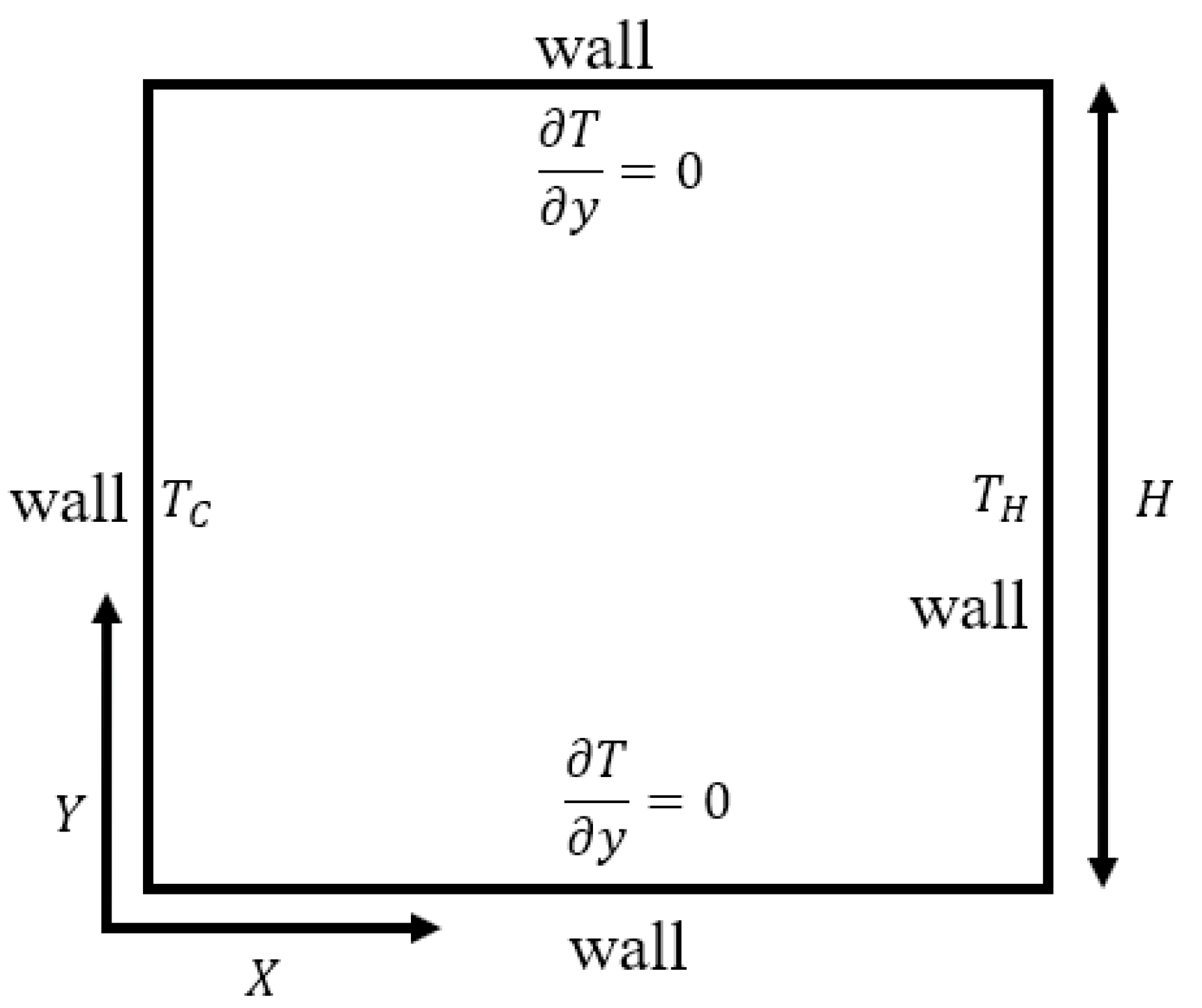
The proposed method, MGLB, was evaluated through the study of a typical example of natural convection in a heated square cavity. The computational domain is shown in Figure 1. The top and the bottom walls are adiabatic while the walls at the left and right are maintained at T_c and T_h, respectively, where $T_H>T_c$. The natural convection inside the cavity can be characterized by the dimensionless numbers $Ra = g\beta \left(T_H-T_c\right)H^3/\alpha \nu$ and $Pr = \nu /\alpha$, where $\beta$ is the thermal expansion coefficient, $\nu$ is the kinematic viscosity of the fluid, and $\alpha$ is the thermal diffusivity. The side length H is the characteristic length of the system. The flow was assumed as Newtonian, laminar, and incompressible, while Boussinesq approximation was applied to model the buoyancy force. The natural convection was simulated for different Pr ranging from 0.01 to 100 for Ra = 10⁶. The governing equations for fluid flow and heat transfer can be written as:

Continuity equation:

$$\frac{\partial \rho }{\partial t}+\rho \nabla ·\mathit{u} = 0$$

(1)

Momentum equation:

$$\rho \left(\frac{\partial \mathit{u}}{\partial t}+\mathit{u}·\nabla \mathit{u}\right) = -\nabla P+\nabla ·\left(\mu \nabla \mathit{u}\right)+\rho \mathit{g}\beta \left(T-\overline{T}\right)$$

(2)

Energy equation:

$$\frac{\partial T}{\partial t}+\mathit{u}·\nabla T = \alpha {\nabla }^{2}T$$

(3)

The Boussinesq approximation states that the fluid properties are constant except for calculating the density in the buoyancy force as $\rho =\overline{\rho }\left(1-\beta \left(T-\overline{T}\right)\right)$;$\overline{\rho }$ and $\overline{T}$ are the average density and temperature, respectively.

In this study, two different distribution functions, $f_{\alpha }\left(\mathit{x},t\right)$ for fluid flow and $g_{\alpha }\left(\mathit{x},t\right)$ for heat transfer, were employed. The transport coefficients were considered temperature-independent, so the fluid flow and energy equation could be solved independently. The system of equations was only coupled through the buoyancy force term in Equation (2). Therefore, not only could the equations be solved with two different numerical techniques, such as the LB method for fluid flow and finite difference for energy equation, but the grid size dx and the time step dt could also be selected differently for fluid flow and energy equations.

In this study, all results are reported in non-dimensional form using the following variables: $\mathrm{X} = x/H$, Y = y/H, $u_c = \sqrt{g\beta \left(T_h-T_h\right)H}$, $U = u_x/u_c$, V = $u_y/u_c$ and $\theta = \frac{T-T_C}{T_H-T_C}$.

The Nusselt number, which is defined as the ratio of convection to conduction, is written as:

$$Nu = {\frac{h}{k/H}|}_{x = H} = {\frac{\partial \theta }{\partial X}|}_{X = H}$$

(4)

where k is thermal conductivity and h is the heat transfer coefficient. The average Nusselt number can be defined as:

$$N{u}_{ave} = {{\displaystyle \int }}_0^1\frac{\partial \theta }{\partial X}dY$$

(5)

In the LB method, the fluid flow is described by the distribution function $f_{\alpha }$, which represents the probability of finding a fictive fluid particle at a given time and location. The particle motion and collision are modeled by the evolution of the distribution function $f_{\alpha }$ in discrete directions. In this work, the D₂Q₉ lattice was used to discretize the velocity space. In the D₂Q₉ lattice, each node at position x has a distribution function $f_{\alpha }\left(\mathit{x},t\right)$ in any of the nine discrete directions ${\mathit{e}}_{\alpha }$, which is defined as:

$$\{\begin{array}{cc}{\mathit{e}}_0 = 0 & \mathrm{for} \alpha = 0\hfill \\ {\mathit{e}}_{\alpha } = \left(\cos \left[\frac{\left(\alpha -1\right)\pi }{2}\right],\sin \left[\frac{\left(\alpha -1\right)\pi }{2}\right]\right)c & \mathrm{for} \alpha = 1,2,3,4\hfill \\ {\mathit{e}}_{\alpha } = \sqrt{2}\left(\cos \left[\frac{\left(\alpha -5\right)\pi }{2}+\frac{\pi }{4}\right],\sin \left[\frac{\left(\alpha -5\right)\pi }{2}+\frac{\pi }{4}\right]\right)c& \mathrm{for} \alpha = 5,6,7,8\hfill \end{array}$$

(6)

where $c = \frac{\mathsf{\Delta }{x}_{LB}}{\mathsf{\Delta }{t}_{LB}} = 1$ is the lattice speed, $\mathsf{\Delta }{x}_{LB} = 1$ is the lattice spacing, and $\mathsf{\Delta }{t}_{LB} = 1$ is the lattice time-step size. The multi-distribution lattice Boltzmann equations for fluid flow and heat transfer in the most general form can be written as:

$$f_{\alpha }\left(\mathit{x}+{\mathit{e}}_{\alpha }\mathsf{\Delta }t,t+\mathsf{\Delta }t\right)-f_{\alpha }\left(\mathit{x},t\right) = {\mathsf{\Omega }}_f+{\mathit{F}}_{\alpha }\left(\mathit{x},t\right)$$

(7)

$$g_{\alpha }\left(\mathit{x}+{\mathit{e}}_{\alpha }\mathsf{\Delta }t,t+\mathsf{\Delta }t\right)-g_{\alpha }\left(\mathit{x},t\right) = {\mathsf{\Omega }}_g$$

(8)

where $f_{\alpha }\left(\mathit{x},t\right)$ and $g_{\alpha }\left(\mathit{x},t\right)$ are density distribution functions and temperature distribution functions, respectively. ${\mathit{F}}_{\alpha }\left(\mathit{x},t\right)$ is the buoyancy force at each grid node. $\mathsf{\Omega }$ is related to modeling the collision step. The simplest model is the linear Bhatnagar–Gross–Krook (BGK) collision model, which is also called the single relaxation time (SRT) and defines the collision terms as:

$${\mathsf{\Omega }}_f = -\frac{1}{{\tau }_f}\left(f_{\alpha }\left(\mathit{x},t\right)-f_{\alpha }^{eq}\left(\mathit{x},t\right)\right)$$

(9)

$${\mathsf{\Omega }}_g = -\frac{1}{{\tau }_g}\left(g_{\alpha }\left(\mathit{x},t\right)-g_{\alpha }^{eq}\left(\mathit{x},t\right)\right)$$

(10)

where ${\tau }_f$ and ${\tau }_g$ are the relaxation times for the fluid flow and temperature field. The relaxation time is related to the LB kinematic viscosity and thermal diffusivity. $c_s$ is the lattice sound speed and for the $D_2{Q}_9$ lattice it is given by $c_s^2 =$1/3 [10].

$${\nu }_{LB,f}=c_s^2{\times (\tau }_f-0.5)$$

(11)

$${\alpha }_{LB,g}=c_s^2{\times (\tau }_g-0.5)$$

(12)

The relaxation time is required to be higher than 0.5 to ensure non-negative kinematic viscosity and thermal diffusivity. The LB kinematic viscosity and thermal diffusivity are related thorough $Pr$ as:

$$Pr = \frac{{\nu }_{LB,f}}{{\alpha }_{LB,g}} = \frac{{\nu }_{ph}}{{\alpha }_{ph}}$$

(13)

where subscripts LB and ph correspond to lattice Boltzmann and physical units, respectively. From Equations (11) to (13), the relaxation time for fluid flow and temperature field are related as:

$${\tau }_g = \frac{{\tau }_f-0.5}{Pr}+0.5$$

(14)

The fluid equilibrium density distribution function in the D₂Q₉ model is defined as:

$$f_{\alpha }^{\mathrm{eq}}={\omega }_{\alpha }\rho \left[1+\frac{3}{{\mathrm{c}}^2}\left(e_{\alpha }·{\mathit{u}}_{\mathit{L}\mathit{B},\mathit{f}}\right)+\frac{9}{2c^4}{\left(e_{\alpha }·{\mathit{u}}_{\mathit{L}\mathit{B},\mathit{f}}\right)}^2-\frac{2}{3c^2}{\mathit{u}}_{\mathit{L}\mathit{B},\mathit{f}}{}^2\right]$$

(15)

Whereas for temperature field it is defined as:

$$g_{\alpha }^{eq}={\omega }_{\alpha }\rho \left[1+\frac{3}{{\mathrm{c}}^2}\left({\mathit{e}}_{\alpha }·{\mathit{u}}_{\mathit{L}\mathit{B},\mathit{g}}\right)\right]$$

(16)

where ${\mathit{u}}_{\mathit{L}\mathit{B},f}$ and ${\mathit{u}}_{\mathit{L}\mathit{B},\mathit{g}}$ are velocity vectors in the lattice units for fluid flow and temperature fields, respectively. If the grids used for fluid flow and temperature calculations are the same, then ${\mathit{u}}_{\mathit{L}\mathit{B},\mathit{f}} = {\mathit{u}}_{\mathit{L}\mathit{B},\mathit{g}}$. Otherwise, velocity must be “converted” to account for the different grids. This will be further discussed in Section 2.1. ${\mathsf{\omega }}_{\alpha }$ is a weight coefficient defined as:

$${\omega }_{\alpha }=\{\begin{array}{c}\frac{4}{9} \alpha = 0\\ \frac{1}{9} \alpha = 1,2,3,4\\ \frac{1}{36} \alpha = 5,6,7,8\end{array}$$

(17)

The macroscopic density, velocity, and temperature at each node are recovered through:

$${\rho }_{LB, f}\left(\mathit{x},t\right) = {\displaystyle \sum }_{\alpha = 0}^9{f}_{\alpha }\left(\mathit{x},t\right)$$

(18)

$${\rho }_{LB, f}\left(\mathit{x},t\right){\mathit{u}}_{\mathit{L}\mathit{B},\mathit{f}}\left(\mathit{x},t\right) = {\displaystyle \sum }_{\alpha = 0}^9{f}_{\alpha }\left(\mathit{x},t\right){\mathit{e}}_{\alpha }$$

(19)

$$\theta \left(\mathit{x},t\right)={\displaystyle \sum }_{\alpha =0}^9{g}_{\alpha }\left(\mathit{x},t\right)$$

(20)

With these settings and through the Chapman–Enskog expansion, Equations (1)–(3) can be recovered [52,53].

The characteristic velocity is an essential parameter to non-dimensionalize the equations. For natural convection problems, the characteristic velocity is usually defined as $u_c = \sqrt{g\beta \mathsf{\Delta }TH}$, where H is the number of grid cells in the x-direction and $\mathsf{\Delta }T$ is the temperature difference between the right and left walls. The value of $u_c$ in LB units should lie within the limit of incompressible flow (Ma = $u_c/c_s$ < 0.3); therefore, it should be less than 0.17 for the D₂Q₉ lattice since the speed of sound $c_s^2 =$1/3. In this study, the characteristic velocity was chosen to be less than 0.1 in all cases to stay far away from the incompressible limit. The kinematic viscosity in lattice units can be calculated from the relation between Ra and Pr numbers, $Ra = u_c^2{H}_{LB,f}^{2}Pr/{\nu }_{LB,f}^2$. Then, the thermal diffusivity is calculated from Equation (13). Once the kinematic viscosity and thermal diffusivity in lattice units are known, both the thermal and fluid relaxation times can be calculated from Equations (11) and (12).

As previously mentioned, both the relaxation times for fluid flow and temperature field should be greater than 0.5 for a physical fluid. Furthermore, it has been shown in the BGK method that the solution is unstable when the relaxation time approaches 0.5. Although there is no upper limit for relaxation time, when recovering the Navier–Stokes equation through the Chapman–Enskog expansion, it is assumed that the distribution function $f_{\alpha }$ is departed from equilibrium through a small perturbation as $f_{\alpha } = f_{\alpha }^{\mathrm{eq}}+\epsilon f_{\alpha }^1+O\left({\epsilon }^2\right)$, where $\epsilon \propto \tau$. As a result, smaller truncation errors can be achieved when relaxation times are less than 1.0. Therefore, in the BGK method, both relaxation times should be in the range (0.5–1] to obtain maximum stability and accuracy [22,24,51,54,55,56]. According to Equations (13) and (14), at very high or very low $Pr$ numbers, the relaxation time for either fluid flow or energy equation becomes $\tau \approx 0.5$ or $\tau \gg 1$. The implicit relation between $Pr$ number and relaxation times, in combination with the incompressible flow constraint, restricts the ability of the SRT model to simulate small or large $Pr$ numbers.

2.1. Multiple-Grid Lattice Boltzmann (MGLB)

The idea behind the proposed method relies on the fact that by choosing different grid sizes and time steps for fluid flow and energy equations, the relaxation times in both equations can be selected separately, resulting in the increase of stability.

The fluid flow equation needs the temperature at each node of the velocity grid to calculate the buoyancy force, while the energy equation needs the velocity at each node of the temperature grid to calculate the advection term in the equilibrium function. The procedure to transfer variables between meshes is explained in this section. Figure 2 shows the position of two arbitrary fine and coarse meshes relative to each other. The following explanation assumes a fine mesh for velocity and a coarse mesh for temperature, and the goal is to transfer temperature from the coarser grid to the finer grid.

If the velocity and temperature grids coincide at a node, the temperature is directly transferred from the temperature grid to the velocity grid. For a non-coincident node in the velocity grid, the four nearest neighboring nodes in the temperature grid are found (as shown in Figure 2). Then the temperature in the velocity node is determined from the interpolation weights, $w_i$, as follows.

$${\theta }_{fine} = w_1{\theta }_A+w_2{\theta }_B+w_3{\theta }_C+w_4{\theta }_D$$

(21)

where ${\theta }_A$ to ${\theta }_D$ are known. The weight coefficients $w_i$ must satisfy the following conditions:

$${\displaystyle \sum }{w}_i=1$$

(22)

$$w_1{d}_1 = w_2{d}_2 = w_3{d}_3 = w_4{d}_4$$

(23)

These conditions provide four equations (one in Equation (22) and three in Equation (23)) for the four unknowns $w_i$. The solutions are:

$$\begin{gathered} w_1 = \frac{1}{1+\frac{d_1}{d_2}+\frac{d_1}{d_3}+\frac{d_1}{d_4}} \\ {w}_2 = \frac{d_1}{d_2}{w}_1 \\ {w}_3 = \frac{d_1}{d_3}{w}_1 \\ {w}_4 = \frac{d_1}{d_4}{w}_1 \end{gathered}$$

(24)

Equations (22) and (24) provide the procedure to transfer the temperature values from the coarse grid to the fine velocity grid. The same technique can be used to transfer the velocity from the fine grid to the coarse temperature grid. It should be noted that the LB method for both velocity and temperature is second-order accurate in space. However, the mapping method for transferring variables between coarse and fine grids, as in Figure 2, is linear, which makes the model first-order accurate. Higher-order interpolation schemes can be used instead of linear interpolation with the drawback of higher computational time. As an example, quadratic interpolation needs 9 neighboring nodes instead of 4 nodes in the linear interpolation. The extra nodes will make the model computationally expensive.

In addition to the previous interpolation procedure to transfer variables between the fine and coarse grids, the variables must also be “converted” to account for the different grids. The conversion between the fine and coarse grids can be achieved by equating the non-dimensional parameters such as Reynolds number ($Re$), Prandtl number (Pr), and/or any combination of non-dimensional numbers between the fine and coarse grids and physical scaling. The non-dimensional diffusion time scales are defined as $t_f^{*} = \frac{\mathsf{\Delta }t\nu }{H^2}$ for fluid domain and $t_g^{*} = \frac{\mathsf{\Delta }t\alpha }{H^2}$ for energy equation. H in the physical unit is defined as the actual length of the domain and in the LB unit is defined as the number of grids along the physical length. By equating the non-dimensional diffusion time scales in physical and LB units, we have:

$$\mathsf{\Delta }{t}_{ph,f} = \frac{{\nu }_{LB,f}}{{\nu }_{ph}}{\left(\frac{H_{ph}}{H_{LB,f}}\right)}^2 = \frac{{\nu }_{LB,f}}{{\nu }_{ph}}{\left(\mathsf{\Delta }{x}_{ph,f}\right)}^2$$

(25)

$$\mathsf{\Delta }{t}_{ph,g} = \frac{{\alpha }_{LB,g}}{{\alpha }_{ph}}{\left(\frac{H_{ph}}{H_{LB,g}}\right)}^2 = \frac{{\alpha }_{LB,g}}{{\alpha }_{ph}}{\left(\mathsf{\Delta }{x}_{ph,g}\right)}^2$$

(26)

By substituting the ${\nu }_{LB,f}$ and ${\alpha }_{LB,g}$ from Equations (25) and (26) into Equations (11) and (12), the relationship between relaxation time and physical properties such as grid size and time step are obtained as:

$${\tau }_f = \frac{3{\nu }_{ph}\mathsf{\Delta }{t}_{ph,f}}{{\left(\mathsf{\Delta }{x}_{ph,f}\right)}^2}+0.5$$

(27)

$${\tau }_g = \frac{3{\alpha }_{ph}\mathsf{\Delta }{t}_{ph,g}}{{\left(\mathsf{\Delta }{x}_{ph,g}\right)}^2}+0.5$$

(28)

By substituting the value of ${\nu }_{ph}$ and ${\alpha }_{ph}$ into the definition of $Pr$, the relation between relaxation time using MGLB can be obtained as:

$${\tau }_g = {\left(\frac{\mathsf{\Delta }{x}_{ph,f}}{\mathsf{\Delta }{x}_{ph,g}}\right)}^2\frac{\mathsf{\Delta }{t}_{ph,g}}{\mathsf{\Delta }{t}_{ph,f}}\frac{{\tau }_f-0.5}{Pr}+0.5$$

(29)

By comparing Equation (29) with Equation (14), it is noted that the value of ${\tau }_g$ is now also a function of grid size and time-step ratios.

The velocities, $u_{LB,f}$ and $u_{LB,g}$, required to calculate the equilibrium distribution function in Equations (15) and (16), are not equal in the MGLB model. To find the relation, the Courant number $Cu = \frac{u\mathsf{\Delta }t}{\mathsf{\Delta }x}$ must be equal in both LB and physical units as:

$$\frac{\mathsf{\Delta }{t}_{ph,f}{u}_{ph}}{\mathsf{\Delta }{x}_{ph,f}} = \frac{\mathsf{\Delta }{t}_{LB,f}{u}_{LB,f}}{\mathsf{\Delta }{x}_{LB,f}}$$

(30)

$$\frac{\mathsf{\Delta }{t}_{ph,g}{u}_{ph}}{\mathsf{\Delta }{x}_{ph,g}} = \frac{\mathsf{\Delta }{t}_{LB,g}{u}_{LB,g}}{\mathsf{\Delta }{x}_{LB,g}}$$

(31)

Since both $\mathsf{\Delta }{t}_{LB}$ and $\mathsf{\Delta }{x}_{LB}$ are equal to 1, by equating the physical velocity in both equations, the relationship between $u_{LB,g}$ and $u_{LB,f}$ is obtained as:

$$u_{LB,g} = \frac{\mathsf{\Delta }{t}_{ph,g}}{\mathsf{\Delta }{t}_{ph,f}}\frac{\mathsf{\Delta }{x}_{ph,f}}{\mathsf{\Delta }{x}_{ph,g}}{u}_{LB,f}$$

(32)

Equations (29) and (32) are written in general form, meaning that it is not implied whether the fine grid is chosen for the fluid flow or the energy equation. The selection of whether the fluid flow or energy equation should have a finer grid depends on the simulation’s goal. If the simulation’s purpose is to capture the small vortexes in the domain, then the velocity field should have a finer grid. However, if the aim of the simulation is to increase the overall stability or to reduce the total computational time, selecting different grid and time steps based on the value of the Pr number can help to alleviate the divergence problem as given by Equation (29). Here we only focus on stability and reducing the computational time issues.

Therefore, for the case of $Pr\ll 1$, when a uniform grid and time step is used, according to Equation (14), ${\tau }_g$ may become very large (${\tau }_{LB,g}\gg 1$). To reduce ${\tau }_g$ by the MGLB method, according to Equation (29), the grid and time step are selected as $\frac{\mathsf{\Delta }{x}_{ph,f}}{\mathsf{\Delta }{x}_{ph,g}}\le 1$ and $\frac{\mathsf{\Delta }{t}_{ph,g}}{\mathsf{\Delta }{t}_{ph,f}}\le 1$. The selection implies that a finer mesh is chosen for fluid flow, while the energy equation has smaller time steps.

The grid ratio (GR) is defined as the ratio of the number of cells in the x-direction of the fine grid to the cell number in the coarse grid. Therefore, for $Pr\ll 1$, it can be written as $GR = \frac{\mathsf{\Delta }{x}_{ph,g}}{\mathsf{\Delta }{x}_{ph,f}} = \frac{H_{LB,f}}{H_{LB,g}}$. The time-step ratio (n) is defined as the ratio of the time step in the finer grid (in this case fluid flow) to the time step in the coarse mesh: n = $\frac{\mathsf{\Delta }{t}_{ph,f}}{\mathsf{\Delta }{t}_{ph,g}}$. The effect of selecting different values for GR and n on stability and computational time will be discussed in the Section 3.

With the same analogy, when $Pr\gg 1$, ${\tau }_g$ could become very small when a uniform grid and time step are used. To increase the ${\tau }_g$ according to Equation(29), the grid size and time step are chosen so that $\frac{\mathsf{\Delta }{x}_{ph,f}}{\mathsf{\Delta }{x}_{ph,g}}\ge 1$ and $\frac{\mathsf{\Delta }{t}_{ph,g}}{\mathsf{\Delta }{t}_{ph,f}}\ge 1$, which means a finer mesh for the energy equation, while having smaller time steps for the fluid-flow model. Here the grid ratio and time-step ratio are defined as $GR = \frac{H_{LB,g}}{H_{LB,f}} = \frac{\mathsf{\Delta }{x}_{ph,f}}{\mathsf{\Delta }{x}_{ph,g}}$ and $\mathrm{n}=\frac{\mathsf{\Delta }{t}_{ph,g}}{\mathsf{\Delta }{t}_{ph,f}}$, respectively.

3. Results

The stability and computational time enhancements of the LB model were tested by simulating natural convection in a side-heated square cavity, as described in Figure 1. Results reveal that the Pr number has a significant effect on the formation of vortices and flow patterns.

3.1. Natural Convection Inside a Heated Square Cavity: Benchmark Test

Initially, the natural convection inside a heated square cavity for Pr = 0.7 (air) was studied. The results obtained with the conventional SRT-LB model were validated against the results reported in references [40,42].

To obtain grid-independent results, several different grid sizes have been examined, and a 400 × 400 grid was selected for both velocity and temperature fields. The streamlines and isotherms obtained with the LB model are plotted in Figure 3, which is in qualitative agreement with [40,42].

The average Nusselt number along the right wall in addition to the maximum velocity location and magnitude were compared with previous studies and listed in

Table 2. Quantitative comparison of Nusselt number and the maximum velocity location and magnitude. The values in parentheses are locations of maximum velocity measured from the cavity center.

	$\mathit{N}{\mathit{u}}_{\mathit{a}\mathit{v}\mathit{e}}$	Umax(y)	Vmax(x)
Current study	8.85	65.03(0.845)	215.8(0.0391)
Ref. [42]	8.7746	64.91(0.8516)	218.90(0.0391)
Ref. [40]	8.8251	64.84(0.8505)	220.46(0.0390)

. A conversion of the current study results to the way references [40,42] reported their results was done for consistency.

These results compare very well with the ones published in [40,42], showing a maximum error of 0.3% for both $N{u}_{ave}$ and velocity, which demonstrates that the SRT-LB method is capable of generating correct results for natural convection for Ra = 10⁶ for Pr = 0.7.

The accuracy of the conventional LB (SRT method) for modeling various Pr numbers was further validated with the results reported in [41,43]. The same 400 × 400 grid was selected as before for both velocity and temperature fields. The results are summarized in

Table 3. Comparison of $N{u}_{ave}$ for different Pr numbers.

$\mathit{N}{\mathit{u}}_{\mathit{a}\mathit{v}\mathit{e}}$	Pr = 0.005 Ra = 15,000	Pr = 0.007 Ra = 105	Pr = 0.01 Ra = 105	Pr = 0.071 Ra = 105	Pr = 0.71 Ra = 105	Pr = 7.1 Ra = 105
Current	2.08	2.65	3.18	3.76	4.45	4.68
Ref. [41]	2.10	N/A	3.23	N/A	N/A	N/A
Ref. [43]	N/A	2.58	N/A	3.80	4.48	4.72

.

For the case Pr = 0.01 and Ra = 10⁵, we report the long-time average of the transient $N{u}_{ave}$ due to the oscillation of temperature in the domain with time. The results of this validation revealed that the conventional SRT-LB method was capable of generating correct results for natural convection in a wide range of Pr, although at the expense of using a very fine mesh.

3.2. Natural Convection with SRT Method for Prandtl Numbers 0.01 and 100

In this section, numerical results for a fine grid with the SRT method at Pr = 0.01 and 100 for Ra = 10⁶ are presented. These results are later used as a reference for calculating the accuracy of the results obtained by the MGLB method.

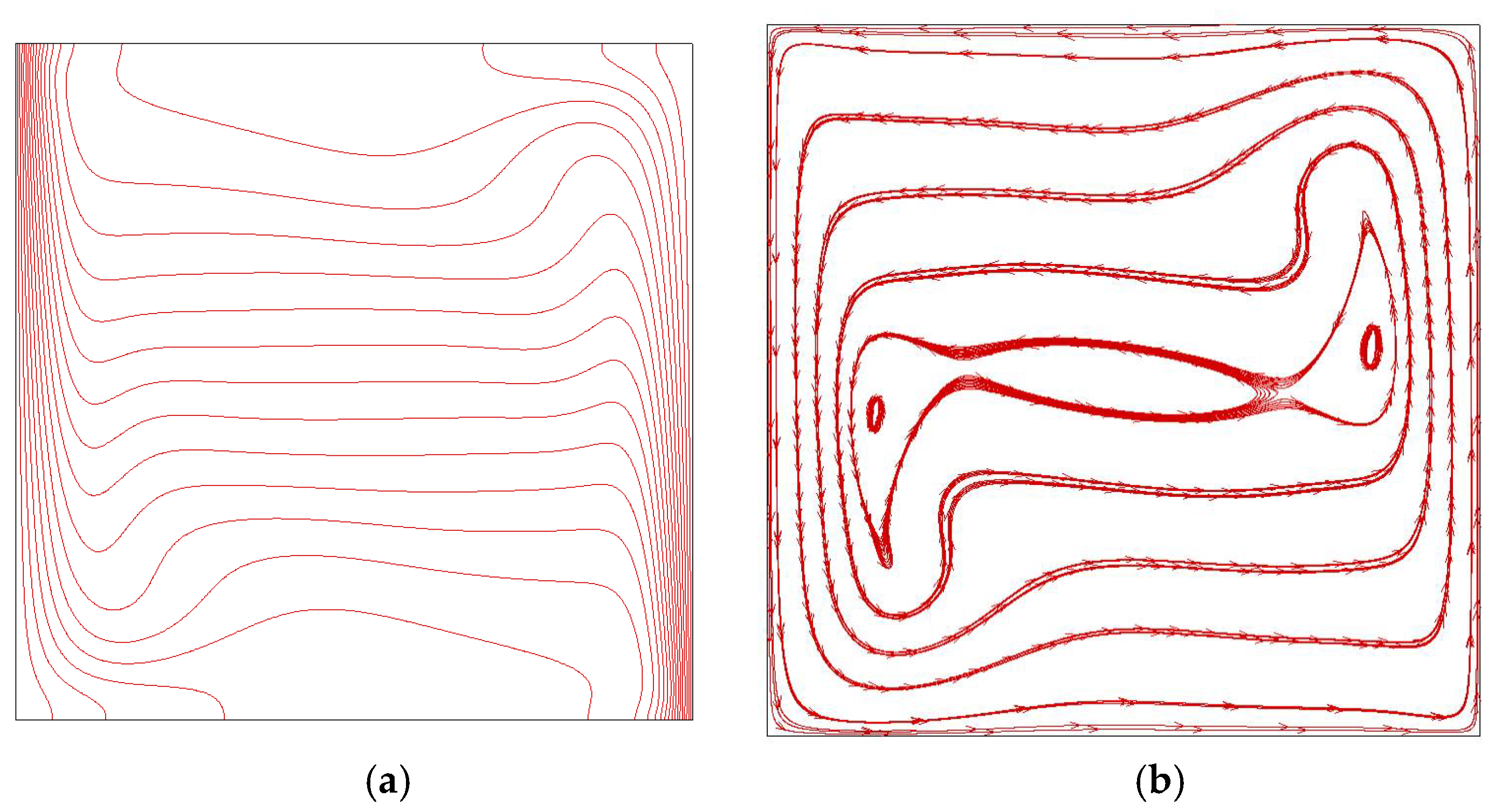
A fine grid of 400 × 400 cells was used for the SRT-LB model to avoid solution divergence and achieve grid-independent results for both Pr = 0.01 and Pr = 100. The streamlines and isotherms are shown in Figure 4. They provide detailed information about the nature of heat transfer. At low Prandtl numbers (Figure 4a,c), flow is dominated by vortices near the center of the cavity. By increasing Pr (Figure 4b,d), the streamlines start to become concentrated near the wall, and flow moves counterclockwise from the hot wall upward. With the increase of Pr, fluid viscosity increases, which eventually causes convection to dominate over conduction in transferring energy.

Figure 5 shows the SRT-LB results of flow velocity and temperature profiles inside the side-heated cavity in the midsection along the vertical and horizontal directions.

For the low Prandtl number (Pr = 0.01), the long-time average of the transient velocity profiles was reported. As other researchers have reported, the solution is oscillatory in the case of a low Prandtl number [6,57]. The results in that case never reach the steady-state. A more detailed description of the unsteady nature of the low Prandtl number results is discussed in Appendix A.

The temperature profile is comparable for all the cases in Figure 5. However, the velocity profile shows that the stability of vortex pairs increases with increasing Pr number. In lower Pr numbers, the breakdown of vortex symmetry is observed, which leads to instability.

3.3. Natural Convection with MGLB Method

In this section, the MGLB model was employed to solve natural convection in the side-heated square cavity with the two extreme values of Prandtl number: 0.01 and 100 for Ra = 10⁶. As will be discussed in this section, unless a very fine mesh is used, numerical instability is observed in the SRT method. This restriction in the $Pr$ number was discussed in detail in Section 2. The effects of selecting different time steps and grid sizes (different values of n and GR) on stability, accuracy, and computational time was investigated extensively. The accuracy of the proposed MGLB method was compared to the fine-grid SRT model presented in Section 3.3.

The low Prandtl number was studied first via twelve cases with input parameters shown in

Table 4. Input parameters and simulation results for $Ra = {10}^6$, $Pr = 0.01$ for simulations with single relaxation time (SRT) (Cases 1 and 2) and multiple-grid lattice Boltzmann (MGLB) (Cases 3 to 12). “N/A” indicates no convergence. The characteristic velocity was selected as $u_c = 0.05$ in all cases. The Time column is normalized by Case 2. The average Nu number from SRT-LB simulations presented in Section 3.2 was 5.312.

Case No.	${\mathit{H}}_{\mathit{f}}$	${\mathit{H}}_{\mathit{g}}$	n	GR	${\mathbf{\tau }}_{\mathit{f}}$	${\mathbf{\tau }}_{\mathit{g}}$	$\mathit{N}{\mathit{u}}_{\mathit{a}\mathit{v}\mathit{e}}$	Time
1(SRT)	100	100	1	1	0.5015	0.6500	N/A	N/A
2(SRT)	200	200	1	1	0.5030	0.8000	5.345	1.000
3(MGLB)	100	100	2	1	0.5015	0.5750	5.105	0.193
4(MGLB)	150	100	1	1.5	0.5023	0.6000	5.350	0.456
5(MGLB)	150	100	2	1.5	0.5023	0.5500	5.343	0.491
6(MGLB)	150	100	3	1.5	0.5023	0.5333	5.350	0.544
7(MGLB)	200	100	1	2	0.5030	0.5750	5.467	0.719
8(MGLB)	200	100	2	2	0.5030	0.5375	5.461	0.737
9(MGLB)	200	100	3	2	0.5030	0.5250	5.455	0.789
10(MGLB)	300	100	1	3	0.5045	0.5500	5.538	1.965
11(MGLB)	300	100	2	3	0.5045	0.5250	5.539	2.000
12(MGLB)	300	100	3	3	0.5045	0.5167	5.535	2.053

. The characteristic velocity, $u_c$, was selected as 0.05 in all cases to satisfy the incompressible limit, as explained in Section 2.1. The average Nusselt number, $N{u}_{ave}$, obtained with MGLB was compared with the average Nu number from SRT-LB simulations presented in Section 3.2, as the reference for error calculation. The error is defined as $error = \left|N{u}_{SRT\_fine}-N{u}_{ave}\right|/N{u}_{SRT\_fine}\times 100$. The first two cases in Table 4 were solved with the SRT method while the rest were solved with the MGLB method. The N/A in the table for Case 1 indicates that the solution diverged due to the coarse grid. By using a finer mesh, as in Case 2, the SRT method did eventually converge. The computational time in each case was calculated and then normalized with respect to the computational time of Case 2. The normalized time is a measure for comparing the computational time between the MGLB and SRT methods. The $N{u}_{ave}$ for all cases was measured, and the error was calculated.

Figure 6 summarizes the results obtained by the SRT and MGLB methods regarding the accuracy and computational time. The horizontal and vertical solid lines define a threshold for error and computational time, respectively. The acceptable error was defined as 10%, while a normalized time of 1 was selected as a threshold for time. These two lines divide the plane into four quadrants, where the points of interest lie above the third quartile. In the third quartile, the computational time and error are acceptable. In all MGLB cases, the simulation converged, with the total number of grid cells being much less than the counterpart SRT method.

Case 1 diverged very quickly due to the coarseness of the mesh. Case 2 converged with a finer mesh while the characteristic velocity $u_c$ remained the same. The simulation time in Case 2 was used as the reference value for comparison with the MGLB method.

Case 3 demonstrates the ability of the MGLB method to increase stability and reduce computational time. While keeping the grid size the same as Case 1, by increasing n (the time-step ratio), the simulation converged with more than 80% reduction in computational time compared to Case 2.

The best result regarding the error was obtained when GR = 1.5, in Cases 4, 5, and 6. When GR = 2, the simulation gets computationally more expensive and the error increases. The increase in error can be explained by the coupling between fluid flow and energy equations. In the SRT method, the grid size and time step are the same, which can be considered a coupling between the two equations. The MGLB method weakens the coupling due to the intermediate interpolation step. For GR = 3, the computational time is higher than for Case 2 even though the total number of grid cells is less than Case 2. Figure 6 also shows that increasing the time-step ratio (n) does not lead to more accurate results. Instead, it improves the stability (compare Cases 1 and 3, for instance). When the simulation diverges for a specific initial parameter and grid size, increasing n might prevent the simulation from diverging. It was also observed that for GR = 1.5, 2, and 3, increasing n only makes the simulation computationally more expensive.

The MGLB model was also applied for a high Prandtl number (Pr = 100), as shown in

Table 5. Input parameters and simulation results for $Ra = {10}^6$, $Pr = 100$ for simulations with SRT (Cases 1 to 3) and MGLB (Cases 4 to 14). “N/A” indicates that the solution diverged. The characteristic velocity was selected as $u_c = 0.05$ in all cases. The average Nu number from SRT-LB simulations presented in Section 3.2 was 9.240.

Case No.	${\mathit{H}}_{\mathit{f}}$	${\mathit{H}}_{\mathit{g}}$	n	GR	${\mathbf{\tau }}_{\mathit{f}}$	${\mathbf{\tau }}_{\mathit{g}}$	$\mathit{N}{\mathit{u}}_{\mathit{a}\mathit{v}\mathit{e}}$	Time
1(SRT)	100	100	1	1	0.6500	0.5015	N/A	N/A
2(SRT)	300	300	1	1	0.950	0.5045	N/A	N/A
3(SRT)	350	350	1	1	1.0250	0.5052	9.2980	1.000
4(MGLB)	100	100	2	1	0.6500	0.5030	N/A	N/A
5(MGLB)	100	100	3	1	0.6500	0.5045	N/A	N/A
6(MGLB)	100	150	1	1.5	0.6500	0.5034	N/A	N/A
7(MGLB)	100	150	2	1.5	0.6500	0.5067	8.523	0.089
8(MGLB)	100	150	3	1.5	0.6500	0.5101	8.521	0.117
9(MGLB)	100	200	1	2	0.6500	0.5060	8.453	0.108
10(MGLB)	100	200	2	2	0.6500	0.5120	8.451	0.141
11(MGLB)	100	200	3	2	0.6500	0.5180	8.450	0.160
12(MGLB)	100	300	1	3	0.6500	0.5135	8.489	0.178
13(MGLB)	100	300	2	3	0.6500	0.5270	8.487	0.239
14(MGLB)	100	300	3	3	0.6500	0.5405	8.486	0.296

. The first three cases were solved with the SRT method. The characteristic velocity was again selected as $u_c = 0.05$ in all cases. Contrary to the cases with low Prandtl numbers, a much finer grid is required to prevent the solution from diverging, as seen in Case 3. It was also checked that the results obtained in case 3 were grid-independent. In Cases 4 and 5, the same grid as Case 1 was used while trying to increase the stability by increasing the time-step ratio. It turns out that the solution still diverges in those cases. Cases 6 through 8 show that increasing the time-step ratio for the same grid ratio GR = 1.5 would help to solve the divergence problem that occurred in Case 6. The computational time was normalized against Case 3.

The error was about 7 to 9% in all cases, as shown in Figure 7. For a high Pr number, the MGLB method successfully reduced the computational time to at least 1/3 of the SRT method. Again, the same trend of increasing the time-step ratio on increasing computational time and error was observed here. For the same GR, increasing the time-step ratio can improve stability, but has no effect on reducing the error.

Compared to the conventional SRT method, the MGLB method offers better stability and computational time with reasonable accuracy.

Based on the MGLB method results for high and low Prandtl numbers, the following procedure is proposed to obtain the least computational time and error.

For both low and high Prandtl numbers, GR = 1.5 yielded optimum results. The time-step ratio in both high and low Prandtl numbers controls the stability. It should be selected as n = 1 initially, and if the solution diverges, a higher value can be chosen.

Nonetheless, the proposed MGLB method reduces the computational time significantly compared to the conventional SRT method. The MGLB method can also be employed with other collision models such as MRT, entropic, or cascaded LB rather than the SRT scheme. The main difference between these methods lies in how the collision operator is modeled, which is not affected by the proposed method.

4. Conclusions

A multiple-grid lattice Boltzmann (MGLB) single relaxation time (SRT) model has been proposed. The model implements a different grid and time step for fluid flow and energy equations. The simulations showed that the model enhances the stability of the standard SRT-LB method while maintaining its simplicity. Solving natural convection problems for extreme values of Prandtl number is particularly challenging in terms of numerical convergence and accuracy. This methodology took care of the problem by selecting an optimal grid and time step for each equation, depending on the value of Pr number. The method was validated against the classic example of natural convection in a side-heated square cavity for Ra = 10⁶ and Pr = 0.7. The results were in good agreement with simulations performed with numerical results reported in the literature. By appropriate selections of the grid and time step, computational savings up to ten-fold could be obtained when compared with the conventional SRT method. Due to the increase in stability, the model was also able to simulate cases for which the SRT method would not even converge. Considering that these were relatively simple 2D simulations, the advantages of the proposed MGLB method are expected to be significantly better when applied to complex 3D problems. Since the MGLB is a general approach, independent of the way the collision is modeled, we expect that it can be successfully implemented for other collision models as well.

References

- Aidun, C.K.; Clausen, J.R. Lattice-Boltzmann Method for Complex Flows. Annu. Rev. Fluid Mech. 2010, 42, 439–472. [Google Scholar] [CrossRef]
- D’Orazio, A.; Corcione, M.; Celata, G.P. Application to Natural Convection Enclosed Flows of a Lattice Boltzmann BGK Model Coupled with a General Purpose Thermal Boundary Condition. Int. J. Therm. Sci. 2004, 43, 575–586. [Google Scholar] [CrossRef]
- Connington, K.; Lee, T. A Review of Spurious Currents in the Lattice Boltzmann Method for Multiphase Flows. J. Mech. Sci. Technol. 2012, 26, 3857–3863. [Google Scholar] [CrossRef]
- He, X.; Luo, L.S. A Priori Derivation of the Lattice Boltzmann Equation. Phys. Rev. E Stat. Phys. Plasmas Fluids Relat. Interdiscip. Top. 1997, 55. [Google Scholar] [CrossRef] [Green Version]
- Shih, H.C.; Huang, C.L. Image Analysis and Interpretation for Semantics Categorization in Baseball Video. Proc. ITCC 2003 Int. Conf. Inf. Technol. Comput. Commun. 2003, 94, 379–383. [Google Scholar] [CrossRef]
- Li, Z.; Yang, M.; Zhang, Y. Double MRT Thermal Lattice Boltzmann Method for Simulating Natural Convection of Low Prandtl Number Fluids. Int. J. Numer. Methods Head Fluid 2016, 26. [Google Scholar] [CrossRef]
- Perumal, D.A.; Dass, A.K. A Review on the Development of Lattice Boltzmann Computation of Macro Fluid Flows and Heat Transfer. Alex. Eng. J. 2015, 54, 955–971. [Google Scholar] [CrossRef] [Green Version]
- McNamara, G.; Alder, B. Analysis of the Lattice Boltzmann Treatment of Hydrodynamics. Phys. A Stat. Mech. Appl. 1993, 194, 218–228. [Google Scholar] [CrossRef]
- Alexander, F.J.; Chen, S.; Sterling, J.D. Lattice Boltzmann Thermohydrodynamics. Phys. Rev. E 1993, 47, R2249–R2252. [Google Scholar] [CrossRef] [PubMed] [Green Version]
- Qian, Y.H. Simulating Thermohydrodynamics with Lattice BGK Models. J. Sci. Comput. 1993, 8, 231–242. [Google Scholar] [CrossRef]
- Nie, X.; Qian, Y.H.; Doolen, G.D.; Chen, S. Lattice Boltzmann Simulation of the Two-Dimensional Rayleigh-Taylor Instability. Phys. Rev. E Stat. Phys. Plasmas Fluids Relat. Interdiscip. Top. 1998, 58, 6861–6864. [Google Scholar] [CrossRef]
- He, X.; Chen, S.; Zhang, R. A Lattice Boltzmann Scheme for Incompressible Multiphase Flow and Its Application in Simulation of Rayleigh-Taylor Instability. J. Comput. Phys. 1999, 152, 642–663. [Google Scholar] [CrossRef]
- McNamara, G.R.; Garcia, A.L.; Alder, B.J. Stabilization of Thermal Lattice Boltzmann Models. J. Stat. Phys. 1995, 81, 395–408. [Google Scholar] [CrossRef]
- Li, Q.; Luo, K.H.; He, Y.L.; Gao, Y.J.; Tao, W.Q. Coupling Lattice Boltzmann Model for Simulation of Thermal Flows on Standard Lattices. Phys. Rev. E Stat. Nonlinear Soft Matter Phys. 2012, 85, 16710. [Google Scholar] [CrossRef] [Green Version]
- Nabavizadeh, S.A.; Talebi, S.; Sefid, M.; Nourmohammadzadeh, M. Natural Convection in a Square Cavity Containing a Sinusoidal Cylinder. Int. J. Therm. Sci. 2012, 51, 112–120. [Google Scholar] [CrossRef]
- Prasianakis, N.I.; Karlin, I.V. Lattice Boltzmann Method for Thermal Flow Simulation on Standard Lattices. Phys. Rev. E Stat. Nonlinear Soft Matter Phys. 2007, 76. [Google Scholar] [CrossRef] [Green Version]
- Fattahi, E.; Farhadi, M.; Sedighi, K. Lattice Boltzmann Simulation of Natural Convection Heat Transfer in Eccentric Annulus. Int. J. Therm. Sci. 2010, 49, 2353–2362. [Google Scholar] [CrossRef]
- Souayeh, B.; Ben-Cheikh, N.; Ben-Beya, B. Numerical Simulation of Three-Dimensional Natural Convection in a Cubic Enclosure Induced by an Isothermally-Heated Circular Cylinder at Different Inclinations. Int. J. Therm. Sci. 2016, 110, 325–339. [Google Scholar] [CrossRef]
- Parmigiani, A.; Huber, C.; Chopard, B.; Latt, J.; Bachmann, O. Application of the Multi Distribution Function Lattice Boltzmann Approach to Thermal Flows. Eur. Phys. J. Spec. Top. 2009, 171, 37–43. [Google Scholar] [CrossRef]
- Dixit, H.N.; Babu, V. Simulation of High Rayleigh Number Natural Convection in a Square Cavity Using the Lattice Boltzmann Method. Int. J. Heat Mass Transf. 2006, 49, 727–739. [Google Scholar] [CrossRef]
- Li, Z.; Yang, M.; Zhang, Y. Lattice Boltzmann Method Simulation of 3-D Natural Convection with Double MRT Model. Int. J. Heat Mass Transf. 2016, 94, 222–238. [Google Scholar] [CrossRef] [Green Version]
- D’Humières, D.; Ginzburg, I.; Krafczyk, M.; Lallemand, P.; Luo, L.S. Multiple-Relaxation-Time Lattice Boltzmann Models in Three Dimensions. Philos. Trans. R. Soc. A Math. Phys. Eng. Sci. 2002, 360, 437–451. [Google Scholar] [CrossRef] [PubMed]
- Wang, J.; Wang, D.; Lallemand, P.; Luo, L.S. Lattice Boltzmann Simulations of Thermal Convective Flows in Two Dimensions. Comp. Math. Appl. 2013, 65, 262–286. [Google Scholar] [CrossRef]
- Contrino, D.; Lallemand, P.; Asinari, P.; Luo, L.S. Lattice-Boltzmann Simulations of the Thermally Driven 2D Square Cavity at High Rayleigh Numbers. J. Comput. Phys. 2014, 275, 257–272. [Google Scholar] [CrossRef] [Green Version]
- Mezrhab, A.; Amine Moussaoui, M.; Jami, M.; Naji, H.; Bouzidi, M. Double MRT Thermal Lattice Boltzmann Method for Simulating Convective Flows. Phys. Lett. Sect. A Gen. At. Solid State Phys. 2010, 374, 3499–3507. [Google Scholar] [CrossRef]
- Xu, A.; Shi, L.; Xi, H.D. Lattice Boltzmann Simulations of Three-Dimensional Thermal Convective Flows at High Rayleigh Number. Int. J. Heat Mass Transf. 2019, 140, 359–370. [Google Scholar] [CrossRef] [Green Version]
- Karlin, I.V.; Ferrante, A.; Öttinger, H.C. Perfect Entropy Functions of the Lattice Boltzmann Method. Europhys. Lett. 1999, 47, 182–188. [Google Scholar] [CrossRef] [Green Version]
- Pareschi, G.; Frapolli, N.; Chikatamarla, S.S.; Karlin, I.V. Conjugate Heat Transfer with the Entropic Lattice Boltzmann Method. Phys. Rev. E 2016, 94. [Google Scholar] [CrossRef] [PubMed]
- Hajabdollahi, F.; Premnath, K.N. Central Moments-Based Cascaded Lattice Boltzmann Method for Thermal Convective Flows in Three-Dimensions. Int. J. Heat Mass Transf. 2018, 120, 838–850. [Google Scholar] [CrossRef] [Green Version]
- Sharma, K.V.; Straka, R.; Tavares, F.W. New Cascaded Thermal Lattice Boltzmann Method for Simulations of Advection-Diffusion and Convective Heat Transfer. Int. J. Therm. Sci. 2017, 118, 259–277. [Google Scholar] [CrossRef]
- Chen, Z.; Shu, C.; Tan, D. A Simplified Thermal Lattice Boltzmann Method without Evolution of Distribution Functions. Int. J. Heat Mass Transf. 2017, 105, 741–757. [Google Scholar] [CrossRef]
- Chen, Z.; Shu, C.; Tan, D.; Wu, C. On Improvements of Simplified and Highly Stable Lattice Boltzmann Method: Formulations, Boundary Treatment, and Stability Analysis. Int. J. Numer. Methods Fluids 2018, 87, 161–179. [Google Scholar] [CrossRef]
- Chen, Z.; Shu, C.; Wang, Y.; Yang, L.M.; Tan, D. A Simplified Lattice Boltzmann Method without Evolution of Distribution Function. Adv. Appl. Math. Mech. 2017, 9, 1–22. [Google Scholar] [CrossRef]
- Chen, Z.; Shu, C.; Tan, D. High-Order Simplified Thermal Lattice Boltzmann Method for Incompressible Thermal Flows. Int. J. Heat Mass Transf. 2018, 127, 1–16. [Google Scholar] [CrossRef]
- Dorari, E.; Eshraghi, M.; Felicelli, S.D. A Multiple-Grid-Time-Step Lattice Boltzmann Method for Transport Phenomena with Dissimilar Time Scales: Application in Dendritic Solidification. Appl. Math. Model. 2018, 62, 580–594. [Google Scholar] [CrossRef]
- Sakane, S.; Takaki, T.; Ohno, M.; Shibuta, Y. Simulation Method Based on Phase-Field Lattice Boltzmann Model for Long-Distance Sedimentation of Single Equiaxed Dendrite. Comput. Mater. Sci. 2019, 164, 39–45. [Google Scholar] [CrossRef]
- López, J.; Gómez, P.; Hernández, J.; Faura, F. A Two-Grid Adaptive Volume of Fluid Approach for Dendritic Solidification. Comput. Fluids 2013, 86, 326–342. [Google Scholar] [CrossRef] [Green Version]
- Sakane, S.; Takaki, T.; Ohno, M.; Shibuta, Y.; Aoki, T. Acceleration of Phase-Field Lattice Boltzmann Simulation of Dendrite Growth with Thermosolutal Convection by the Multi-GPUs Parallel Computation with Multiple Mesh and Time Step Method. Model. Simul. Mater. Sci. Eng. 2019, 27. [Google Scholar] [CrossRef]
- Nabavizadeh, S.A.; Eshraghi, M.; Felicelli, S.D. A Comparative Study of Multiphase Lattice Boltzmann Methods for Bubble-Dendrite Interaction during Solidification of Alloys. Appl. Sci. 2018, 9, 57. [Google Scholar] [CrossRef] [Green Version]
- Hortmann, M.; Perić, M.; Scheuerer, G. Finite Volume Multigrid Prediction of Laminar Natural Convection: Benchmark Solutions. Int. J. Numer. Methods Fluids 1990, 11, 189–207. [Google Scholar] [CrossRef]
- Mohamad, A.A.; Viskanta, R. Transient Natural Convection of Low-Prandtl-number Fluids in a Differentially Heated Cavity. Int. J. Numer. Methods Fluids 1991, 13, 61–81. [Google Scholar] [CrossRef]
- Guo, Z.; Zheng, C.; Shi, B.; Zhao, T.S. Thermal Lattice Boltzmann Equation for Low Mach Number Flows: Decoupling Model. Phys. Rev. E Stat. Nonlinear Soft Matter Phys. 2007, 75. [Google Scholar] [CrossRef]
- Pesso, T.; Piva, S. Laminar Natural Convection in a Square Cavity: Low Prandtl Numbers and Large Density Differences. Int. J. Heat Mass Transf. 2009, 52, 1036–1043. [Google Scholar] [CrossRef]
- Ahlers, G.; Xu, X. Prandtl-Number Dependence of Heat Transport in Turbulent Rayleigh-Bénard Convection. Phys. Rev. Lett. 2001, 86, 3320–3323. [Google Scholar] [CrossRef] [PubMed] [Green Version]
- Kao, P.H.; Yang, R.J. Simulating Oscillatory Flows in Rayleigh-Bénard Convection Using the Lattice Boltzmann Method. Int. J. Heat Mass Transf. 2007, 50, 3315–3328. [Google Scholar] [CrossRef]
- Silano, G.; Sreenivasan, K.R.; Verzicco, R. Numerical Simulations of Rayleigh-Bénard Convection for Prandtl Numbers between 101 and 104 and Rayleigh Numbers between 105 and 109. J. Fluid Mech. 2010, 662, 409–446. [Google Scholar] [CrossRef]
- Fei, L.; Luo, K.H. Cascaded Lattice Boltzmann Method for Thermal Flows on Standard Lattices. Int. J. Therm. Sci. 2018, 132, 368–377. [Google Scholar] [CrossRef]
- Pandey, A.; Scheel, J.D.; Schumacher, J. Turbulent Superstructures in Rayleigh-Bénard Convection. Nat. Commun. 2018, 9. [Google Scholar] [CrossRef] [Green Version]
- De Vahl Davis, G. Natural Convection of Air in a Square Cavity: A Bench Mark Numerical Solution. Int. J. Numer. Methods Fluids 1983, 3, 249–264. [Google Scholar] [CrossRef]
- Bessonov, O.A.; Brailovskaya, V.A.; Nikitin, S.A.; Polezhaev, V.I. Three-Dimensional Natural Convection in a Cubical Enclosure: A Bench Mark Numerical Solution. In Proceedings of the International Symposium on Advances in Computational Heat Transfer, Çesme, Turkey, 26–30 May 1997. [Google Scholar] [CrossRef]
- Guo, Z.; Shi, B.; Zheng, C. A Coupled Lattice BGK Model for the Boussinesq Equations. Int. J. Numer. Methods Fluids 2002, 39, 325–342. [Google Scholar] [CrossRef]
- Qian, Y.H.; D’Humières, D.; Lallemand, P. Lattice Bgk Models for Navier-Stokes Equation. EPL 1992, 17, 479–484. [Google Scholar] [CrossRef]
- Benzi, R.; Succi, S.; Vergassola, M. The Lattice Boltzmann Equation: Theory and Applications. Phys. Rep. 1992, 145–197. [Google Scholar] [CrossRef]
- Luo, L.S.; Liao, W.; Chen, X.; Peng, Y.; Zhang, W. Numerics of the Lattice Boltzmann Method: Effects of Collision Models on the Lattice Boltzmann Simulations. Phys. Rev. E Stat. Nonlinear Soft Matter Phys. 2011, 83. [Google Scholar] [CrossRef] [PubMed] [Green Version]
- Pan, C.; Luo, L.S.; Miller, C.T. An Evaluation of Lattice Boltzmann Schemes for Porous Medium Flow Simulation. Comput. Fluids 2006, 35, 898–909. [Google Scholar] [CrossRef]
- Zhao, F. Optimal Relaxation Collisions for Lattice Boltzmann Methods. Comput. Math. Appl. 2013, 65, 172–185. [Google Scholar] [CrossRef]
- Li, Z.; Yang, M.; Zhang, Y. Numerical Simulation of Melting Problems Using the Lattice Boltzmann Method with the Interfacial Tracking Method. Numer. Heat Transf. Part. A Appl. 2015, 68, 1175–1197. [Google Scholar] [CrossRef]
Figure 1.
Boundary conditions for natural convection in a side-heated square cavity.
Figure 2.
Mapping from the coarse grid (temperature) to the fine grid (fluid flow) (a). The properties at any node in the fine grid are determined from the four nearest neighbor nodes of the coarse grid (b).
Figure 3.
Natural convection in a side-heated cavity for Pr = 0.7 at Ra = 106 obtained with the lattice Boltzmann (LB) model: (a) isotherms and (b) streamlines.
Figure 4.
Isotherms (a,b) and streamlines (c,d) for different with . The results for Pr = 0.01 are reported for Fourier number, Fo = 3.0.
Figure 5.
Non-dimensional velocity in x-direction (a,d), in y-direction (b,e) and temperature profiles (c,f) along the midsection of the cavity (X = 1/2 and Y = 1/2) for different Prandtl numbers and Ra = 106. All the results for Pr = 0.7 and Pr = 100 are reported in steady-state conditions, while for Pr = 0.01, the results are reported for a long-time average of the transient velocity profiles.
Figure 6.
Effect of grid ratio (GR) and n on computational time and error for Pr = 0.01.
Figure 7.
Effect of GR and n on computational time and error for Pr = 100.