Article

Oscillating Magnetohydrodynamic Stokes Flow between Porous Plates with Spatiotemporally Periodic Reabsorption

by
Anastasios Raptis
1,
Christos Manopoulos
1,
Michalis Xenos
2,* and
Sokrates Tsangaris
1
1
School of Mechanical Engineering, National Technical University of Athens, 9 Heroon Polytechniou Str., Zografou, 15780 Athens, Greece
2
Department of Mathematics, University of Ioannina, 45110 Ioannina, Greece
*
Author to whom correspondence should be addressed.
Submission received: 19 February 2021 / Revised: 2 April 2021 / Accepted: 11 April 2021 / Published: 14 April 2021
(This article belongs to the Special Issue Fluids in Magnetic/Electric Fields)

Abstract

:
The study addresses the oscillating magnetohydrodynamic (MHD) Stokes flow between two parallel plates with periodic reabsorption both spatially and temporally. Two cases are distinguished by applying either (1) transverse or (2) parallel external magnetic field. Analytical solutions of velocity and pressure are derived for both cases and the effect of Womersley and Hartmann number, and the absorption coefficient is examined. The study generalizes existing literature on analytic MHD Stokes flow solutions accounting for periodic boundary conditions both in time and space. The non-oscillating non-MHD Stokes flow in a porous channel (available in the literature) is proven to be a limit of the analytic solution introduced here. The MHD effects are noticeable in flows oscillating with low or moderate frequency but are barely detectable in high-frequency flows even in the presence of strong magnetic fields.

1. Introduction

Magnetohydrodynamics (MHD) is the study of electrically conducting fluids moving through magnetic fields. A historical reference in the MHD field is the seminal paper by Hartman [1], who followed the evidence from an electromagnetic pump (previously devised by himself) that led him to this novel field of investigation. The theory of MHD, as disclosed by Hartman [1] and further enriched by Hartman and Lazarus [2], consisted of the classic hydrodynamical equations combined with the general equations of electrodynamics. Later, Swedish physicist Hannes Alfvén received the Nobel Prize for officially initiating the field of MHD by introducing the full set of Navier–Stokes equations combined with the Maxwell’s equations [3].
The attention in the present study is concentrated on low-Reynolds pulsatile flows, which come with interesting features. The theory predicts that high-frequency oscillatory channel flows acquire a boundary-layer character with peak velocity migrating closer to the wall with the increase of Womersley number [4]. Early in the previous century, even before the theoretical foundation of oscillatory flows, Richardson and Tyler conducted experiments on alternating air flows observing the relocation of maximum velocity toward the boundary [5]. Other experimental studies on oscillatory flows in pipes or other geometries cover a range of frequencies spanning (1) the quasi-steady, (2) intermediate, and (3) inertia-dominated regimes [6,7,8]. The pulsatile flows are not only interesting from a scientific perspective but have a direct implication in modern telecommunication industry, which is in need of efficient liquid-cooling microchannels [9]. While the standard Poiseuille flow is self-similar and bound to the Nusselt number, the low-Reynolds pulsatile flow presents with an enhanced thermal performance, which has been confirmed experimentally [10]. An interesting possibility appears if an electrically conducting fluid is chosen as the medium, as an external magnetic field permits the adjustment of the flow profiles. Our knowledge though about MHD oscillatory flows derives mainly from analytical or numerical studies, which usually focalize on biological applications, while the experimental validation is still pending. An overview of bio-MHD theory and its applications in pulsatile biological flows (mainly blood) is available in the literature [11].
A wide range of numerical methods have been employed for the solution of the full MHD problem [12]. On the other hand, the search for analytic solutions is traditionally an important topic because analytic solutions represent the ground truth, thus enabling an accurate view of the underlying physics with minimum computational cost. Moreover, they are useful in the evaluation of numerical schemes and solvers. Analytic solutions can be hard to obtain, which is why they are scarce in the literature. In the field of oscillatory MHD flows, the analytic studies in the literature mainly refer to low-Reynolds flow regimes governed by Stokes equations. Ganesh et al. [13] presented an analytical solution of oscillating MHD Stokes flow under an external transverse magnetic field considering porous plates with steady suction. Malathy et al. [14] studied the pulsatile MHD flow in permeable beds by distinguishing the steady and oscillatory components of the solution. Kahshan et al. [15] accounted for the slip boundary condition and seepage velocity through the walls to investigate steady-state MHD flow in permeable channels with application to hemodialyzers. The case of dusty fluid with an angular velocity was studied by Delhi Babu et al. [16] to examine potential MHD effects considering periodic absorption through the walls.
The present study provides an analytic solution of velocity and pressure fields for the oscillatory MHD creeping flow considering periodic absorption both temporally and spatially, generalizing existing analytic solutions in the literature. The derivation is based on the mathematical approach also followed by Ganesh et al. [13] and Haroon et al. [17]. The analytic solution provided by the latter on steady (non-MHD) Stokes flow with periodic reabsorption proves to be a limit of the analytic solution introduced here. The flow behavior is visualized and analyzed under the effect of various parameters such as Womersley and Hartmann number, and the absorption coefficient.

2. Mathematical Analysis

2.1. Physical Problem and Governing Equations

The physical problem is sketched in Figure 1, graphically depicting the periodically reabsorbing symmetrically placed and parallel porous plates, and the application of a uniform external magnetic field in the y- or x-direction (transverse or parallel case, respectively). The fluid is electrically conducting, incompressible, and Newtonian. The induced magnetic field is considered negligible for MHD flows with a low magnetic Reynolds number.
The oscillating MHD creeping flow is governed by the Stokes equations including Lorentz Force either in (i) x-momentum equation, representing the transverse magnetic field case, or (ii) in the y-momentum, representing the parallel case (which is presented in Appendix A). Thus, for the transverse magnetic field case, the governing equations in two dimensions utilizing the Cartesian coordinate system ( x , y ) are:
ρ u t = p x + μ ( 2 u x 2 + 2 u y 2 ) σ e B o 2 u
ρ v t = p y + μ ( 2 v x 2 + 2 v y 2 )
u x + v y = 0
where ( u , v ) are the velocity components at the x - and y -direction respectively, p is the pressure, μ is the dynamic viscosity, σ e is the electrical conductivity of the fluid, and B o is the magnitude of magnetic induction. The porous plates with spatially and temporally sinusoidal reabsorption are modeled via the velocity boundary conditions,
u ( x , ± b , t ) = 0 , v ( x , ± b , t ) = ± v o s i n ( a x ) s i n ( ω t )
where v o is the characteristic reabsorption velocity. By the introduction of stream function via u = Ψ y   and   v = Ψ x , the system is reduced to a single partial differential equation (PDE),
ρ t ( 2 Ψ x 2 + 2 Ψ y 2 ) = μ ( 4 Ψ x 4 + 2 4 Ψ x 2 y 2 + 4 Ψ y 4 ) σ e B o 2 2 Ψ y 2 .

2.2. Velocity Calculation

It is meaningful to make the following Ansatz,
Ψ ( x , y , t ) = F ( y ) c o s ( a x ) e i ω t
and write the boundary conditions in complex form,
u ( x , ± b , t ) = 0
v ( x , ± b , t ) = ± v o s i n ( a x ) e i ω t ,
noticing that the final solution will eventually be a complex function. The velocity boundary conditions are derived in terms of the function F utilizing Equation (6),
u = d F ( y ) d y c o s ( a x ) e i ω t ( 7 a )   { d F ( b ) d y = 0 d F ( b ) d y = 0 v = a F ( y ) s i n ( a x ) e i ω t ( 7 b )   { F ( b ) = v o a F ( b ) = v o a .
The following dimensionless variables are introduced,
x ¯ = x b , y ¯ = y b , τ = t ω , Ψ ¯ = Ψ b v o , u ¯ = u v o = Ψ ¯ y ¯ , v ¯ = v v o = Ψ ¯ x ¯ , ε = a b , γ = b ρ ω μ , M = σ e B o 2 b 2 μ
where M is the magnetic parameter, which is associated to the Hartmann number H through the formula, M = H 2 . The governing equation is redefined as follows,
γ 2 τ ( 2 Ψ ¯ x ¯ 2 + 2 Ψ ¯ y ¯ 2 ) = 4 Ψ ¯ x ¯ 4 + 2 4 Ψ ¯ x ¯ 2 y ¯ 2 + 4 Ψ ¯ y ¯ 4 M 2 Ψ ¯ y ¯ 2 .
Utilizing the non-dimensional variables (9), the Ansatz is alternatively expressed as,
Ψ ¯ ( x ¯ , y ¯ , τ ) = f ( y ¯ ) c o s ( ε x ¯ ) e i τ .
Substituting Equation (11) in Equation (10), the governing equation reduces to an ordinary differential equation (ODE),
d 4 f d y ¯ 4 ( 2 ε 2 + i γ 2 + M ) d 2 f d y ¯ 2 + ( ε 4 + i γ 2 ε 2 ) f = 0
with the corresponding boundary conditions,
u ¯ = Ψ ¯ y ¯ = d f ( y ¯ ) d y ¯ c o s ( ε x ¯ ) e i τ   u ¯ ( x ¯ , ± 1 , τ ) = 0     { d f ( 1 ) d y ¯ = 0 d f ( 1 ) d y ¯ = 0 v ¯ = Ψ ¯ x ¯ = ε f ( y ¯ ) s i n ( ε x ¯ ) e i τ v ¯ ( x ¯ , ± 1 , τ ) = ± s i n ( ε x ¯ ) e i τ   { f ( 1 ) = 1 ε f ( 1 ) = 1 ε .
The 4th-order homogenous ODE with constant coefficients has the characteristic equation,
λ 4 ( 2 ε 2 + i γ 2 + M ) λ 2 + ( ε 4 + i γ 2 ε 2 ) = 0
with the following roots,
λ = ± 2 ε 2 + i γ 2 + M ± ( M + i γ 2 ) 2 + 4 ε 2 M 2 .
More specifically,
λ 1 = 2 ε 2 + i γ 2 + M + ( M + i γ 2 ) 2 + 4 ε 2 M 2 = λ 2
λ 3 = 2 ε 2 + i γ 2 + M ( M + i γ 2 ) 2 + 4 ε 2 M 2 = λ 4 .
Based on the methods of characteristics, the solution is of the form,
f ( y ¯ ) = c 1 e λ 1 y ¯ + c 2 e λ 1 y ¯ + c 3 e λ 3 y ¯ + c 4 e λ 3 y ¯ .
The constants c 1 ,   c 2 ,   c 3 ,   c 4 are determined by introducing the boundary conditions, Equations (16) and (17), in Equation (18),
c 1 = 1 2 ε λ 3 c o s h ( λ 3 ) λ 3 s i n h ( λ 1 ) c o s h ( λ 3 ) λ 1 c o s h ( λ 1 ) s i n h ( λ 3 ) = c 2
c 3 = 1 2 ε λ 1 c o s h ( λ 1 ) λ 3 s i n h ( λ 1 ) c o s h ( λ 3 ) λ 1 c o s h ( λ 1 ) s i n h ( λ 3 ) = c 4 .
Substituting the constants, Equations (19) and (20), in Equation (18), the analytic solutions of the stream function and the velocity components are derived,
Ψ ¯ ( x ¯ , y ¯ , τ ) = 1 ε λ 3 c o s h ( λ 3 ) s i n h ( λ 1 y ¯ ) λ 1 c o s h ( λ 1 ) s i n h ( λ 3 y ¯ ) λ 3 c o s h ( λ 3 ) s i n h ( λ 1 ) λ 1 c o s h ( λ 1 ) s i n h ( λ 3 ) c o s ( ε x ¯ ) e i τ
u ¯ ( x ¯ , y ¯ , τ ) = λ 1 λ 3 ε c o s h ( λ 3 ) c o s h ( λ 1 y ¯ ) c o s h ( λ 1 ) c o s h ( λ 3 y ¯ ) λ 3 c o s h ( λ 3 ) s i n h ( λ 1 ) λ 1 c o s h ( λ 1 ) s i n h ( λ 3 ) c o s ( ε x ¯ ) e i τ
v ¯ ( x ¯ , y ¯ , τ ) = λ 3 c o s h ( λ 3 ) s i n h ( λ 1 y ¯ ) λ 1 c o s h ( λ 1 ) s i n h ( λ 3 y ¯ ) λ 3 c o s h ( λ 3 ) s i n h ( λ 1 ) λ 1 c o s h ( λ 1 ) s i n h ( λ 3 ) s i n ( ε x ¯ ) e i τ .
The mean velocity and flow rate formulas are
u ¯ m ( x ¯ , τ ) = 1 ε c o s ( ε x ¯ ) e i τ
Q ( x ¯ , τ ) = 1 ε c o s ( ε x ¯ ) e i τ .

2.3. Pressure Calculation

Restructuring the governing equations, Equations (1) and (2), we get the following system in terms of the stream function,
p x = ρ 2 Ψ y t + μ y ( 2 Ψ x 2 + 2 Ψ y 2 ) σ e B o 2 Ψ y
p y = ρ 2 Ψ x t μ x ( 2 Ψ x 2 + 2 Ψ y 2 )
closed with the following boundary condition for pressure,
p ( x , 0 , t )   = 0 .
In addition to the non-dimensional variables in Equation (9), the following pressure-related non-dimensional variables are introduced,
p ¯ = p P , P = μ v o b
and the system (26)–(28) is rewritten,
p ¯ x ¯ = γ 2 2 Ψ ¯ y ¯ τ + y ¯ ( 2 Ψ ¯ x ¯ 2 + 2 Ψ ¯ y ¯ 2 ) M Ψ ¯ y ¯
p ¯ y ¯ = γ 2 2 Ψ ¯ x ¯ τ x ¯ ( 2 Ψ ¯ x ¯ 2 + 2 Ψ ¯ y ¯ 2 )
p ¯ ( x ¯ , 0 , τ ) = 0 .
Introducing the Ansatz, Equation (11), in the above system, we get,
p ¯ x ¯ = [ ( γ 2 i + ε 2 + M ) d f d y ¯ + d 3 f d y ¯ 3 ] c o s ( ε x ¯ ) e i τ
p ¯ y ¯ = ε [ ( γ 2 i + ε 2 ) f + d 2 f d y ¯ 2 ] s i n ( ε x ¯ ) e i τ .
Integrating Equation (33) with respect to x ¯ , followed by differentiation with respect to y ¯ ,
p ¯ = 1 ε [ ( γ 2 i + ε 2 + M ) d f d y ¯ + d 3 f d y ¯ 3 ] s i n ( ε x ¯ ) e i τ + c ( y ¯ , τ )
p ¯ y ¯ = 1 ε [ ( γ 2 i + ε 2 ) d 2 f d y ¯ 2 + d 4 f d y ¯ 4 ] s i n ( ε x ¯ ) e i τ + c ( y ¯ , τ ) y ¯ .
Using Equations (34) and (36) we get c ( y ¯ , τ ) y ¯   =   0 . So, we arrive to the expression of p ¯ appended by a constant c , which remains to be found,
p ¯ = 1 ε [ ( γ 2 i + ε 2 + M ) d f d y ¯ + d 3 f d y ¯ 3 ] s i n ( ε x ¯ ) e i τ + c .
The following expression is retrieved after substituting the known function f in Equation (37),
p ¯ = λ 1 λ 3 ε 2 c o s h ( λ 3 ) c o s h ( λ 1 y ¯ ) [ λ 1 2 ( ε 2 + i γ 2 + M ) ] c o s h ( λ 1 ) c o s h ( λ 3 y ¯ ) [ λ 3 2 ( ε 2 + i γ 2 + M ) ] λ 3 s i n h ( λ 1 ) c o s h ( λ 3 ) λ 1 c o s h ( λ 1 ) s i n h ( λ 3 ) s i n ( ε x ¯ ) e i τ + c .
An equivalent expression emerges if we choose to repeat the process (integration–differentiation) starting with Equation (34) instead of Equation (33). Introducing the boundary condition, Equation (32), the analytic solution of pressure is derived,
p ¯ = 1 λ 1 λ 3 λ 3 2 c o s h ( λ 3 ) [ c o s h ( λ 1 y ¯ ) 1 ] [ λ 1 2 ( ε 2 + i γ 2 ) ] λ 1 2 c o s h ( λ 1 ) [ c o s h ( λ 3 y ¯ ) 1 ] [ λ 3 2 ( ε 2 + i γ 2 ) ] λ 3 s i n h ( λ 1 ) c o s h ( λ 3 ) λ 1 c o s h ( λ 1 ) s i n h ( λ 3 ) s i n ( ε x ¯ ) e i τ .
The steady Stokes flow results by Haroon et al. [17] can be retrieved by taking the limit γ 0 of the analytic solutions, Equations (23), (24), and (39), and setting M = 0 .

3. Results and Discussion

The flow conditions are studied under the effect of parameters: ε , γ , and M . The absorption coefficient ε relates to the spatial reabsorption through the porous walls, Womersley number γ controls the pulsatile flow frequency, and the magnetic parameter M tunes the intensity of the magnetic field.
Figure 2 and Figure 3 display the streamlines on top of velocity magnitude contours for the transverse and the parallel case, in the presence of a magnetic field with increasing intensity, Μ = { 0 , 10 , 100 } . The oscillatory flow is a result of the spatiotemporally periodic reabsorption and its interaction with the magnetic field. For the representation of the flow in Figure 2 and Figure 3, we used the imaginary part of the complex solution, Equations (2) and (3), as mandated by the boundary conditions in the real plane, Equation (4). In the transverse case (Figure 2), the flow is decelerated with the increase of the magnetic field intensity. The deceleration is caused by the Lorentz Force, which removes momentum in the x-direction of the flow when the magnetic field acts normal to it. Conversely, when the magnetic field acts in parallel (Figure 3), the maximum velocity of the fluid does not alter; rather, a restructuring of the flow is mostly observed, especially for Μ = 100 . In both cases, the central jet seems to be flattening, even splitting in multiple jets with the increase of magnetic field intensity. Last but not least, we note that the stability of the solution for different values of the parameters is not addressed in this study. However, we direct the interested reader to the studies by Von Kerczek et al. [18] (on oscillating flow in a non-porous channel), and by Potter and Kutchey [19] (on Hartmann–Poiseuille flow), which prove that flow stabilizes with the increase of Womersley or Hartmann numbers.
To get a deeper insight of the flow behavior, the amplitude ( U ¯ a m p ,   V ¯ a m p , P ¯ a m p )   and phase angle ( φ x ,   φ y , φ p )   indexes are plotted for various combinations of the parameters in the following ranges: ε   =   { 1 , 2 } ,   γ =   { 1 , 5 , 10 } ,   Μ = { 0 , 10 , 100 } , both for the transverse, Figure 4, Figure 5, Figure 6, Figure 7, Figure 8 and Figure 9, and the parallel case, Figure 10, Figure 11, Figure 12, Figure 13, Figure 14 and Figure 15. The indexes are calculated as follows: Starting from the solution of the u ¯ velocity component, as shown in Equation (22), we utilize the part of the expression that is a function of y ¯ and write it in the form of a typical complex number,
U ¯ ( y ¯ ) = λ 1 λ 3 ε c o s h ( λ 3 ) c o s h ( λ 1 y ¯ ) c o s h ( λ 1 ) c o s h ( λ 3 y ¯ ) λ 3 c o s h ( λ 3 ) s i n h ( λ 1 ) λ 1 c o s h ( λ 1 ) s i n h ( λ 3 ) = U ¯ R + i U ¯ I .
Substituting the complex number, Equation (40), back in the solution, Equation (22), the resulting expression is,
u ¯ = ( U ¯ R + i U ¯ I ) c o s ( ε x ¯ ) e i τ = ( U ¯ R + i U ¯ I ) c o s ( ε x ¯ ) [ c o s ( τ ) + i s i n ( τ ) ] = = [ U R ¯ c o s ( τ ) U I ¯ s i n ( τ ) ] c o s ( ε x ¯ ) + i [ U ¯ R s i n ( τ ) + U ¯ I c o s ( τ ) ] c o s ( ε x ¯ ) .
Utilizing the imaginary part of Equation (41), u ¯ is written in terms of U ¯ a m p   and φ x ,
u ¯ = U ¯ a m p s i n ( τ + φ x ) c o s ( ε x ¯ )   w h e r e   U ¯ a m p = U ¯ R 2 + U ¯ I 2 , tan ( φ x ) = U ¯ I U ¯ R
while the mean values of velocity amplitude and phase angle are given by
U ¯ m = 1 ε , φ x , m = 0 .
The next three paragraphs discuss the effect of the parameters ε and γ, without accounting for the magnetic field, thus considering Μ = 0 . For low values of Womersley number γ , a quasi-steady U ¯ a m p emerges with its maximum value converging to U ¯ a m p 2 ε s i n h ( ε ) s i n h ( 2 ε ) 2   , and the phase angle converging to φ x = 0 , f o r   γ 0 . The results are in agreement with the steady case without magnetic field published by Haroon et al. [17]. For low values both of parameter γ and ε, the maximum value converges to   U ¯ a m p 1.5 / ε ( γ 0 ,   ε 0 ). The amplitudes and phase angles of the v ¯ and p ¯ are derived in a similar way.
For high values of Womersley number ( γ ), U ¯ a m p is endowed by all the characteristics of oscillatory flow in a straight tube without porous walls [20]. Specifically, U ¯ a m p presents with a flattened inviscid-flow-like profile at the center of the channel converging to the value, U ¯ a m p 1 s i n h ( ε )   f o r   γ and to the value, U ¯ a m p U ¯ m = 1 ε   for ε 0 . The maximum U ¯ a m p value is attained near the walls where a boundary layer forms, as presented by [20], while φ x approaches the value π 4 at the wall for γ (Figure 5 and Figure 11).
The V ¯ a m p increases monotonically from the center toward the wall of the channel (Figure 6 and Figure 12), and the same applies to P ¯ a m p (Figure 8 and Figure 14). The φ y takes negative values both for low and high γ values but increases as an absolute value with the increase of ε (Figure 7 and Figure 13). The P ¯ a m p increases with the increase of γ (Figure 8 and Figure 14), while φ p is small for low γ values. For high γ values, φ p approaches the value π 2 (Figure 9 and Figure 15).
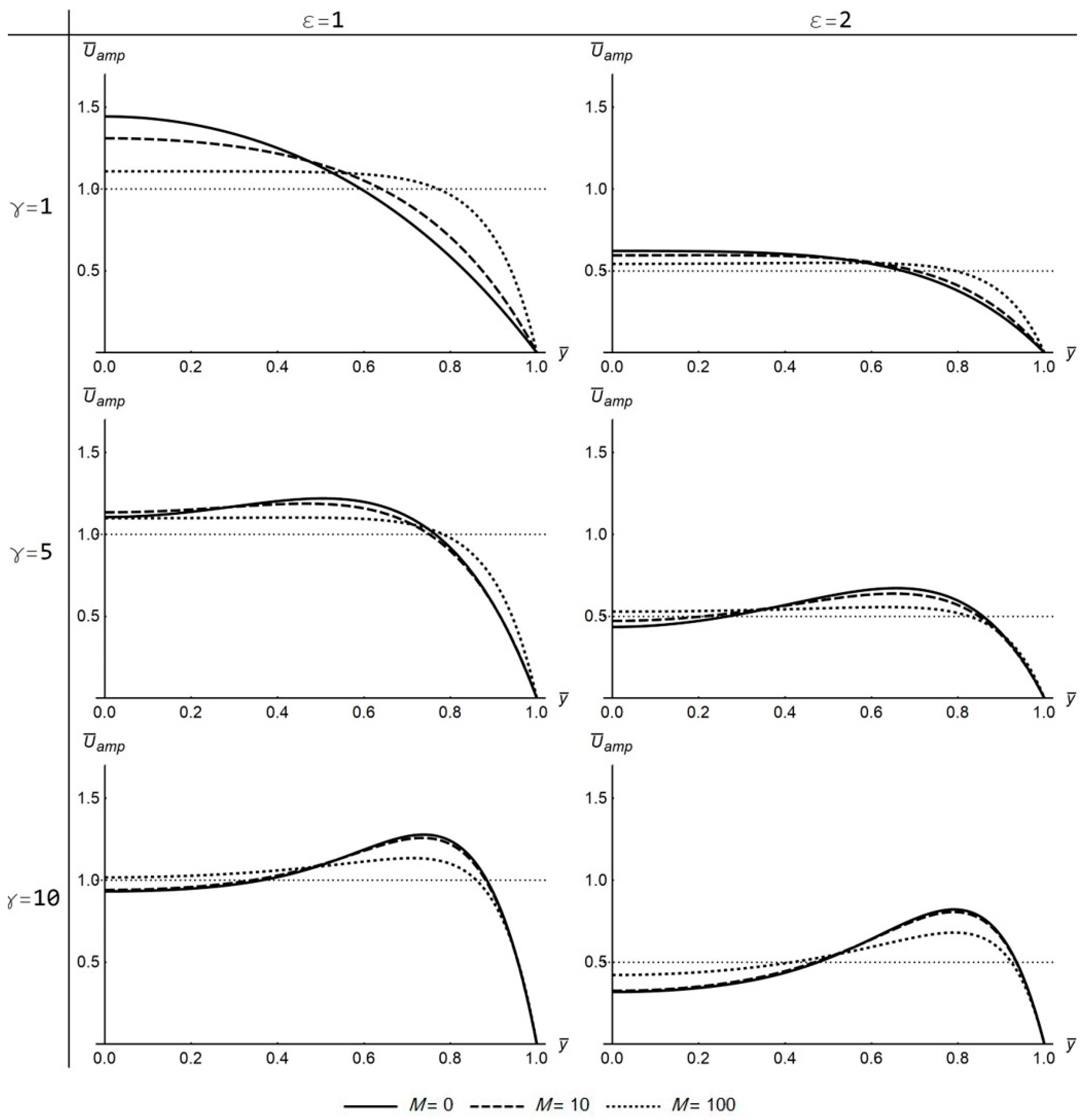
The direction and magnitude of magnetic field has a traceable effect on the amplitude and the phase angle of the flow variables. Concerning the transverse case, the U ¯ a m p profile is further flattening around the center of the channel with the increase of magnetic field intensity, irrespective of ε and γ (Figure 4). However, near the wall, the intensification of magnetic field leads to an increase of U ¯ a m p for low γ values but to a slight decrease for high γ values. On the other hand, for high ε values, the spread between U ¯ a m p profiles for increasing M values is reduced, suggesting that the effect of the magnetic field is alleviated with the increase of absorption coefficient 
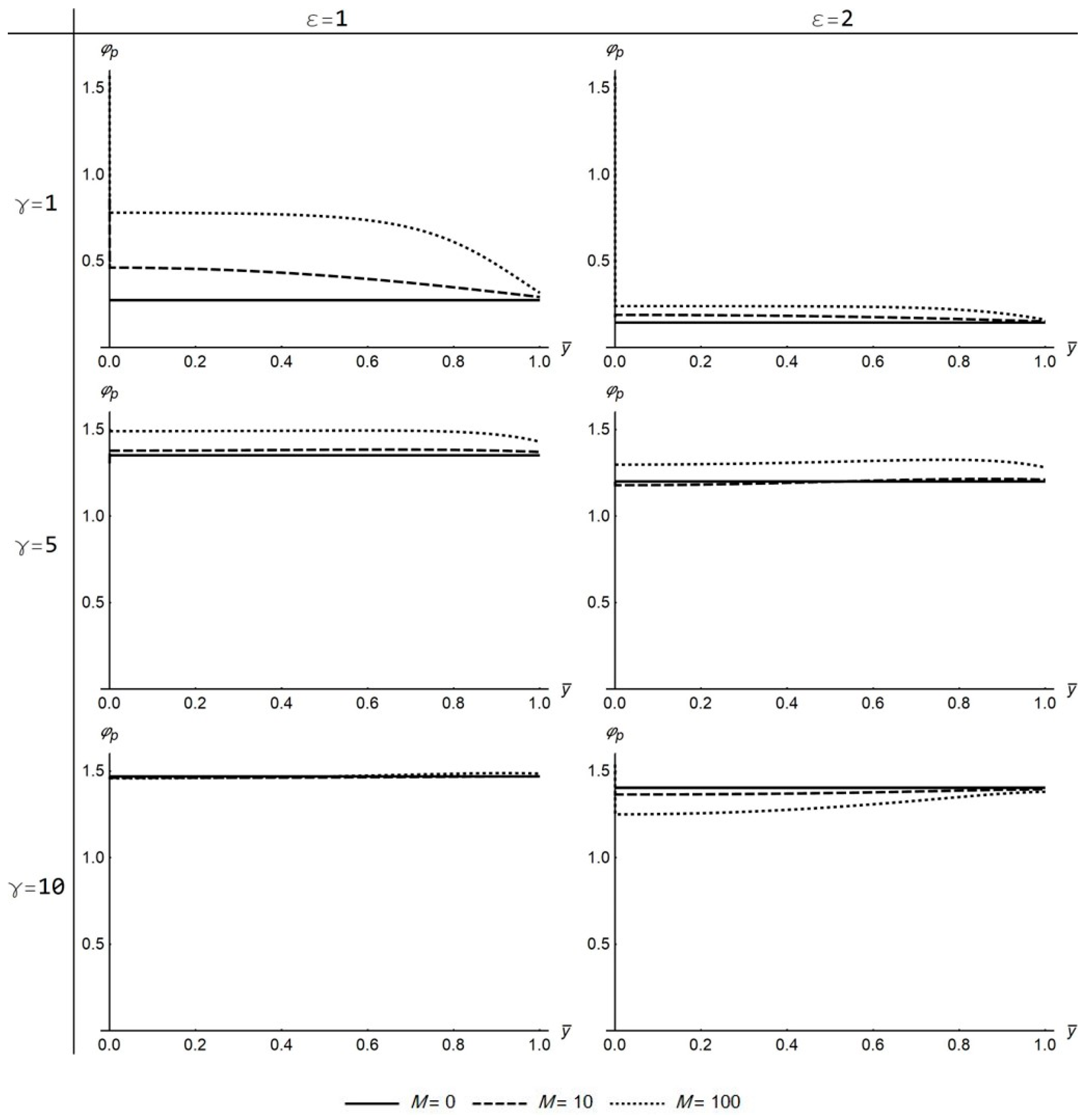
ε. On the other hand, the V ¯ a m p profiles do not alter drastically under the presence of stronger magnetic fields (Figure 6). A noticeable difference between U ¯ a m p and V ¯ a m p profiles with increasing M values is that V ¯ a m p slightly decreases for low γ values but slightly increases for high γ values.
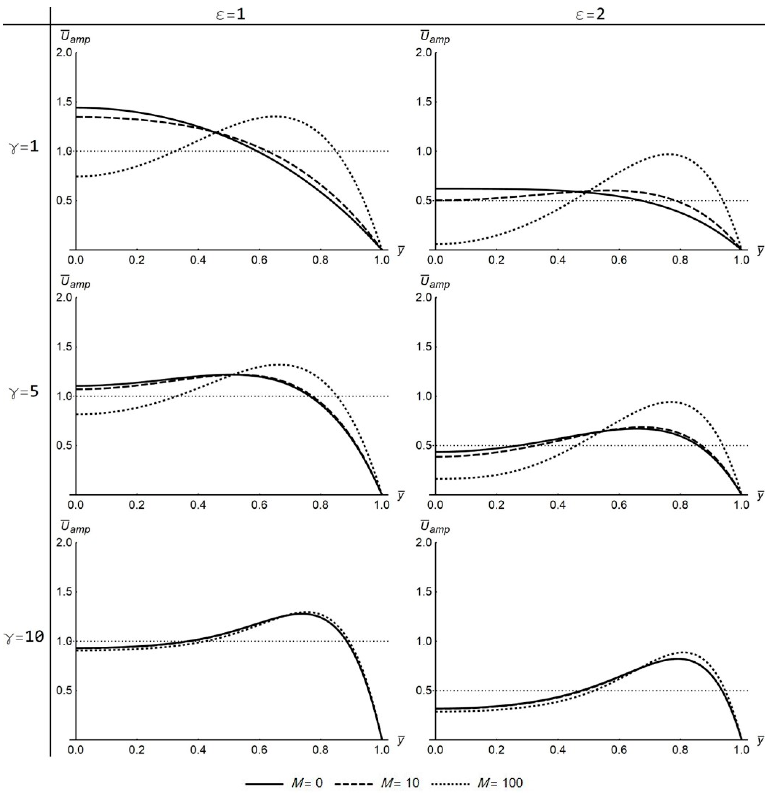
The parallel magnetic field case distinguishes from the transverse at several points, but still some effects are shared between them. Here, the increase of magnetic field intensity reduces U ¯ a m p near the center and reinforces it near the wall, which is noticeable especially for low γ values (Figure 10). For high γ values, the magnetic field does not have a significant effect on U ¯ a m p , even at high intensity, which is a similarity between the parallel (Figure 10) and the transverse case (
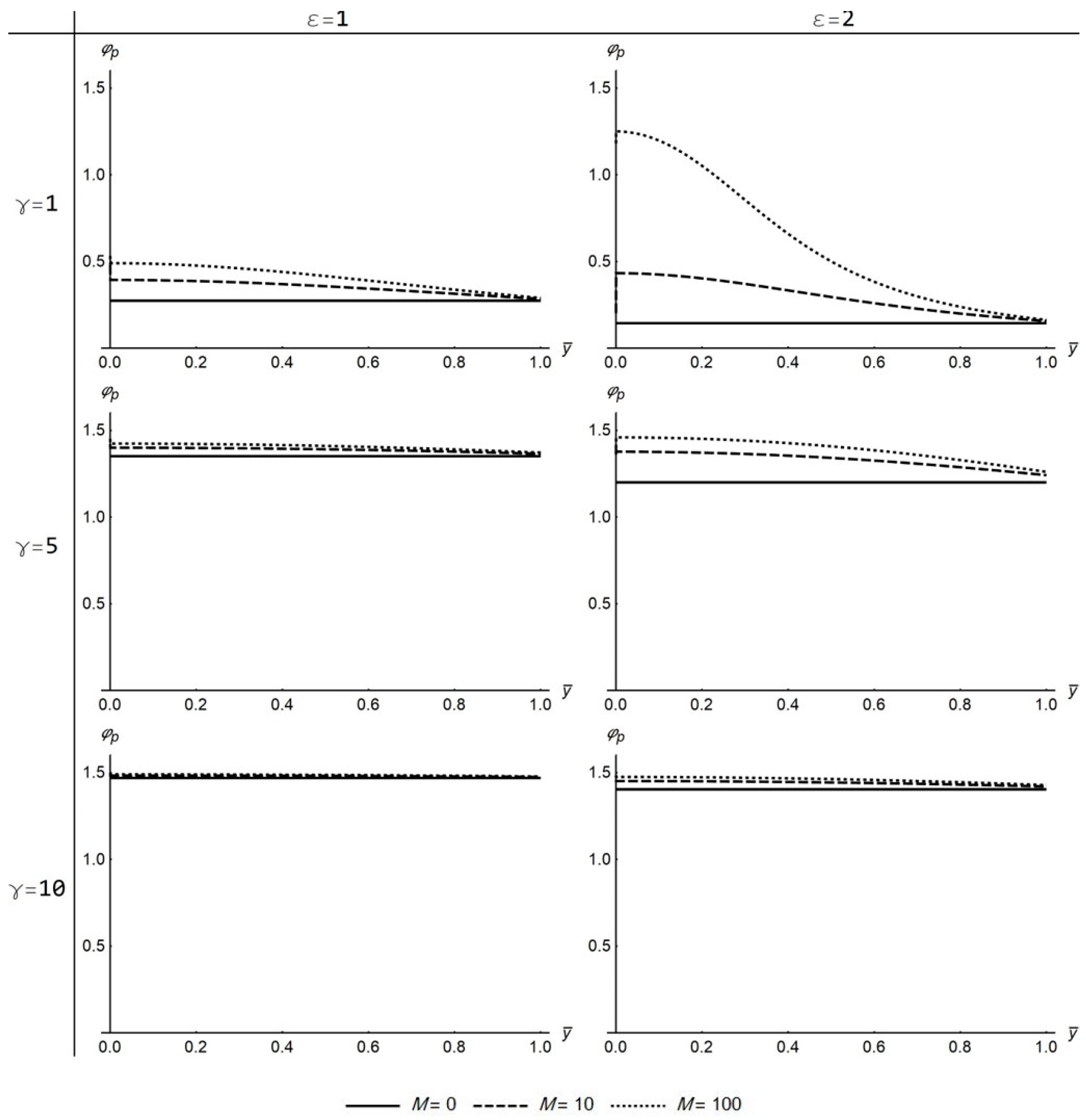
Figure 4). The biggest impact of the parallel magnetic field is concentrated on V ¯ a m p that reduces with the increase of magnetic field intensity (Figure 12). For high ε values, the decrease of V ¯ a m p is even more striking when increasing the intensity of the magnetic field. In contrast to the transverse case, the P ¯ a m p also reduces under stronger parallel magnetic fields, but the decrease is small, even at the highest magnetic intensity (Figure 14). In general, the amplitude of the flow variables for high γ values is not overly sensitive to the magnetic field, even at high intensities, independent of its direction. Seemingly, the high frequency oscillation neutralizes the effects of the magnetic field on the flow.

4. Conclusions and Perspectives

The literature presents only a few analytical solutions on the oscillating MHD Stokes flow. In this study, we introduce an analytical solution that generalizes the existing literature, considering the creeping flow of an electrically conducting fluid in a porous channel in the presence of a magnetic field. The velocity and pressure profiles are drawn for different values of the Womersley and Hartmann numbers as well as the absorption coefficient. The results highlight that the magnetic field casts its biggest impact on the oscillatory flow when the pulsation frequency is low. In high-frequency flows, the MHD effects are not discernible even in the presence of strong magnetic fields. The low-Reynolds pulsatile flows have desirable features and are considered in industrial applications. Additional features are revealed if the typical fluid is replaced by an electrically conducting one that can be controlled by an external magnetic field. More studies, on a theoretical or experimental basis, are required to better understand and take advantage of oscillating MHD flows.

Author Contributions

Conceptualization, S.T.; methodology, S.T.; software, A.R.; validation, A.R., C.M. and M.X.; formal analysis, C.M., M.X. and S.T.; writing—original draft preparation, A.R., C.M., M.X. and S.T.; writing—review and editing, A.R., C.M., M.X. and S.T.; visualization, A.R.; supervision, C.M. and S.T.; project administration, M.X.; All authors have read and agreed to the published version of the manuscript.

Funding

This research is co-financed by Greece and the European Union (European Social Fund-ESF) through the Operational Programme «Human Resources Development, Education and Lifelong Learning» in the context of the project “Reinforcement of Postdoctoral Researchers-2nd Cycle” (MIS-5033021), implemented by the State Scholarships Foundation (ΙΚΥ).
Fluids 06 00156 i001

Institutional Review Board Statement

Not applicable.

Data Availability Statement

Not applicable.

Conflicts of Interest

The authors declare no conflict of interest.

Appendix A

Appendix A.1. Velocity Solution

The governing equations in the parallel magnetic field case are:
ρ u t = p x + μ ( 2 u x 2 + 2 u y 2 )
ρ v t = p y + μ ( 2 v x 2 + 2 v y 2 ) σ e B o 2 v
u x + v y = 0
with the same boundary conditions as in the transverse case, as shown in Equation (4).
With the introduction of the stream function, the system reduces to the PDE:
ρ t ( 2 Ψ x 2 + 2 Ψ y 2 ) = μ ( 4 Ψ x 4 + 2 4 Ψ x 2 y 2 + 4 Ψ y 4 ) σ e B o 2 2 Ψ x 2 .
Introducing the non-dimensional variables, Equations (9), and the Ansatz, Equation (27), in Equation (A4), the PDE reduces to an ODE in terms of the still unknown function f :
d 4 f d y ¯ 4 ( 2 ε 2 + i γ 2 ) d 2 f d y ¯ 2 + ( ε 4 + i γ 2 ε 2 + M ε 2 ) f = 0 .
The ODE is solved by the method of characteristics. The roots of the characteristic equations are
λ = ± 2 ε 2 + i γ 2 ± i γ 4 + 4 ε 2 M 2 .
Hereafter, the expressions of the constants,   c 1 ,   c 2 ,   c 3 ,   c 4 and the final analytic solutions of the stream function and the velocity components are exactly the same with the transverse magnetic field case. The two cases differentiate only in the expressions of the constants,   λ 1 ,   λ 2 ,   λ 3 ,   λ 4 .

Appendix A.2. Pressure Solution

The pressure is calculated based on the following reformulated set of equations,
ρ u t = p x + μ ( 2 u x 2 + 2 u y 2 )
ρ v t = p y + μ ( 2 v x 2 + 2 v y 2 ) σ e B o 2 v
along with the boundary condition, as in the transverse magnetic field case, as shown in Equation (30). Introducing the non-dimensional variables, Equations (9) and (12), and the Ansatz, Equation (11), the above system is reformulated as follows,
p ¯ x ¯ = [ ( γ 2 i + ε 2 ) d f d y ¯ + d 3 f d y ¯ 3 ] c o s ( ε x ¯ ) e i τ
p ¯ y ¯ = ε [ ( γ 2 i + ε 2 + M ) f + d 2 f d y ¯ 2 ] s i n ( ε x ¯ ) e i τ .
The final solution of pressure for the parallel magnetic field case is the same as for the transverse case, as shown in Equation (39), differentiating only in the definition of λ 1 ,   λ 2 ,   λ 3 ,   λ 4 constants, Equation (A6) in the former and Equation (15) in the latter case.

References

  1. Hartmann, J. Hg-dynamics I. Theory of laminar flow of an electrically conductive liquid in a homogeneous magnetic field. Mat. Fys. Medd. 1937, 15, 1–28. [Google Scholar]
  2. Hartmann, J.; Lazarus, F. Hg-dynamics II. Theory of laminar flow of electrically conductive liquids in a homogeneous magnetic field. Mat. Fys. Medd. 1937, 15, 1–45. [Google Scholar]
  3. Alfvén, H. Existence of electromagnetic-hydrodynamic waves. Nature 1942, 150, 405–406. [Google Scholar] [CrossRef]
  4. Schlichting, H.; Gersten, K. Boundary-Layer Theory, 9th ed.; Springer: Berlin/Heidelberg, Germany, 2017. [Google Scholar]
  5. Richardson, E.; Tyler, E. The transverse velocity gradient near the mouths of pipes in which an alternating or continuous flow of air is established. Proc. Phys. Soc. 1929, 42, 1. [Google Scholar] [CrossRef] [PubMed]
  6. Denison, E.; Stevenson, W. Oscillatory flow measurements with a directionally sensitive laser velocimeter. Rev. Sci. Instrum. 1970, 41, 1475–1478. [Google Scholar] [CrossRef]
  7. Einav, S.; Lee, S.L. Migration in an oscillatory flow of a laminar suspension measured by laser anemometry. Exp. Fluids 1988, 6, 273–279. [Google Scholar] [CrossRef]
  8. Ünsal, B.; Ray, S.; Durst, F.; Ertunç, Ö. Pulsating laminar pipe flows with sinusoidal mass flux variations. Fluid Dyn. Res. 2005, 37, 317. [Google Scholar] [CrossRef]
  9. Persoons, T.; Saenen, T.; Van Oevelen, T.; Baelmans, M. Effect of flow pulsation on the heat transfer performance of a minichannel heat sink. J. Heat Trans. 2012, 134, 091702. [Google Scholar] [CrossRef]
  10. Blythman, R.; Persoons, T.; Jeffers, N.; Nolan, K.; Murray, D. Localised dynamics of laminar pulsatile flow in a rectangular channel. Int. J. Heat Fluid Flow 2017, 66, 8–17. [Google Scholar] [CrossRef]
  11. Rashidi, S.; Esfahani, J.A.; Maskaniyan, M. Applications of magnetohydrodynamics in biological systems-a review on the numerical studies. J. Magn. Magn. Mater. 2017, 439, 358–372. [Google Scholar] [CrossRef]
  12. Bég, O.A. Numerical methods for multi-physical magnetohydrodynamics. J. Magnetohydrodyn. Plasma Space Res. 2013, 18, 93–203. [Google Scholar]
  13. Ganesh, S.; Krishnambal, S. Unsteady Magnetohydrodynamic stokes flow of viscous fluid between two parallel porous plates. J. Appl. Sci. 2007, 7, 374–379. [Google Scholar] [CrossRef] [Green Version]
  14. Malathy, T.; Srinivas, S. Pulsating flow of a hydromagnetic fluid between permeable beds. Int. Commun. Heat Mass Transf. 2008, 35, 681–688. [Google Scholar] [CrossRef]
  15. Kahshan, M.; Lu, D.; Rahimi-Gorji, M. Hydrodynamical study of flow in a permeable channel: Application to flat plate dialyzer. Int. J. Hydrog. Energy 2019, 44, 17041–17047. [Google Scholar] [CrossRef]
  16. Delhi Babu, R.; Ganesh, S.; Kirubhashankar, C. An exact solution of Unsteady Magnetohydrodynamic flow of Dusty fluid between parallel porous plates with an angular velocity. Int. J. Ambient Energy 2020, 1–7. [Google Scholar] [CrossRef]
  17. Haroon, T.; Siddiqui, A.M.; Shahzad, A. Stokes flow through a slit with periodic reabsorption: An application to renal tubule. Alex. Eng. J. 2016, 55, 1799–1810. [Google Scholar] [CrossRef] [Green Version]
  18. Von Kerczek, C.H. The instability of oscillatory plane Poiseuille flow. J. Fluid Mech. 1982, 116, 91–114. [Google Scholar] [CrossRef]
  19. Potter, M.C.; Kutchey, J.A. Stability of plane Hartmann flow subject to a transverse magnetic field. Phys. Fluids 1973, 16, 1848–1851. [Google Scholar] [CrossRef]
  20. Drake, D. On the flow in a channel due to a periodic pressure gradient. Q. J. Mech. Appl. Math. 1965, 18, 1–10. [Google Scholar] [CrossRef]
Figure 1. A sketch of the problem depicting the periodically reabsorbing porous plates and the uniform magnetic field in the y-direction (transverse case) or x-direction (parallel case).
Fluids 06 00156 g001
Figure 2. Velocity stream density plots for the transverse case in various time instances, τ = { 0 ,   π 4 ,   π 2 ,   3 π 4 ,   π } , and Magnetic numbers, Μ = { 0 , 10 , 100 } assuming ε = 1 and γ = 1 .
Fluids 06 00156 g002
Figure 3. Velocity stream density plots for the parallel case in various time instances, τ = { 0 ,   π 4 ,   π 2 ,   3 π 4 ,   π } , and Magnetic numbers, M = { 0 , 10 , 100 } , assuming ε = 1 and γ = 1 .
Fluids 06 00156 g003
Figure 4. The profiles of U ¯ a m p under the effect of ε , γ ,   a n d   M parameters (transverse case).
Fluids 06 00156 g004
Figure 5. The profiles of φ x for different values of the ε , γ ,   and   M parameters (transverse case).
Fluids 06 00156 g005
Figure 6. The profiles of V ¯ a m p for different values of the ε , γ ,   a n d   M parameters (transverse case).
Fluids 06 00156 g006
Figure 7. The profiles of φ y for different values of the ε , γ ,   and   M parameters (transverse case).
Fluids 06 00156 g007
Figure 8. The profiles of P ¯ a m p for different values of the ε , γ ,   and   M parameters (transverse case).
Fluids 06 00156 g008
Figure 9. The profiles of φ p for different values of the ε , γ ,   and   M parameters (transverse case).
Fluids 06 00156 g009
Figure 10. The profiles of U ¯ a m p under the effect of ε , γ ,   a n d   M parameters (parallel case).
Fluids 06 00156 g010
Figure 11. The profiles of φ x for different values of the ε , γ ,   a n d   M parameters (parallel case).
Fluids 06 00156 g011
Figure 12. The profiles of V ¯ a m p for different values of the ε , γ ,   a n d   M parameters (parallel case).
Fluids 06 00156 g012
Figure 13. The profiles of φ y for different values of the ε , γ ,   and   M parameters (parallel case).
Fluids 06 00156 g013
Figure 14. The profiles of P ¯ a m p for different values of the ε , γ ,   and   M parameters (parallel case).
Fluids 06 00156 g014
Figure 15. The profiles of φ p for different values of the ε , γ ,   and   M parameters (parallel case).
Fluids 06 00156 g015
Publisher’s Note: MDPI stays neutral with regard to jurisdictional claims in published maps and institutional affiliations.

