
An Analytical Solution for Unsteady Laminar Flow in Tubes with a Tapered Wall Thickness


Department of Mechanical Engineering, University of Saskatchewan, Saskatoon, SK S7N 5A9, Canada
*
Author to whom correspondence should be addressed.
Fluids 2021, 6(5), 170; https://0-doi-org.brum.beds.ac.uk/10.3390/fluids6050170
Submission received: 1 April 2021
/
Revised: 14 April 2021
/
Accepted: 19 April 2021
/
Published: 23 April 2021
(This article belongs to the Special Issue Unsteady Flows in Pipes)
Abstract
:Transient fluid flows through tubes are critical in such topics as water hammer, ram pumps and pipeline dynamics. While analytical solutions exist in the literature for simple geometries such as tapered and non-tapered tube diameters, one area that is lacking is the case where the wave speed changes along the length. An example of this is a flexible pipe with a tapered wall thickness. In order to calculate the transient pressure response of such a system, this previously required a computationally expensive gridded method of characteristics (MOC) solution. This paper describes an analytical solution to the dynamic laminar flow of liquid in a tube where the wave speed varies along its length. This frequency-domain solution includes frequency-dependent friction effects. A comparison to a method of characteristics (MOC) solution is used to verify the solution. The paper also discusses some numerical issues and provides an approximate method that can be used for high-frequency calculations where limited numerical precision can cause errors. Finally, a preliminary comparison of the computational performance is presented, in which the new method is an order of magnitude faster to calculate than an MOC solution.
1. Introduction
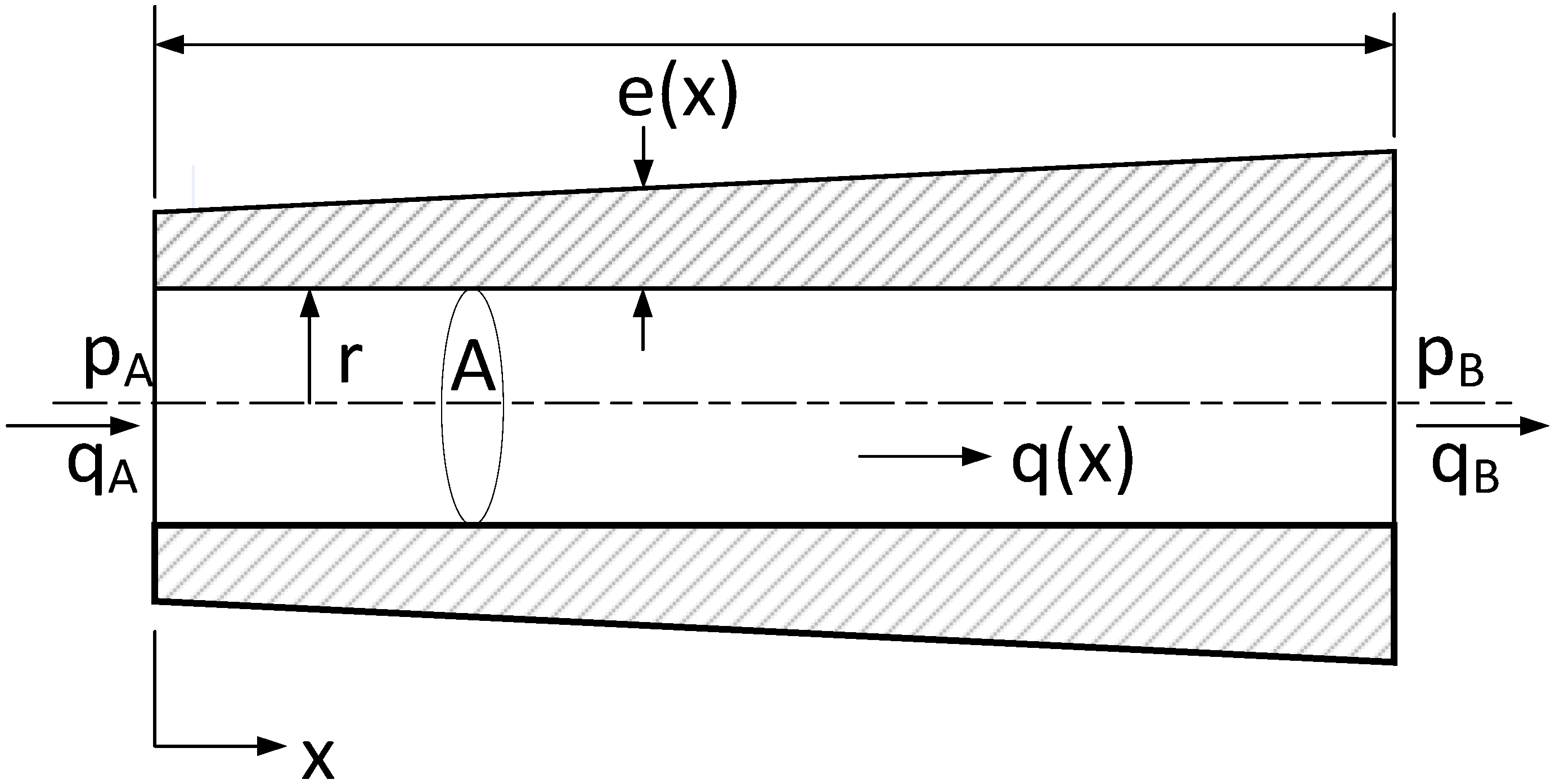
This paper describes an analytical solution for pressure and flow dynamics for laminar liquid flow within a circular tube with constant inner diameter and varying wave propagation speed along its length, as shown in Figure 1. Fluid wave speed inside a non-rigid tube is dependent on the mechanical properties and the geometry of the tube as well as the fluid properties. Considering the pressure wave propagation along a tube, mechanical defects such as erosion, corrosion, and leakage have significant effects on the dynamic response of the pressure and flow. The motivation for this research is the use of such dynamic effects to allow for estimation of the remaining wall thickness in an eroded pipe at a lower cost than existing inspection techniques such as ultrasonic inspection, fiber-optic monitoring or “smart pigs” [1,2,3]. Other applications of this model would include research into water hammer [4], ram pumps [5,6,7], switched inertance hydraulic converters [8,9,10,11] and transient flow measurement [12].
The frequency-domain solution method presented here is computationally faster than existing gridded methods (such as the method of characteristics [13]), as it only calculates pressure and/or flow at the end-points of the tube. It can also be expected to be more accurate than time-domain solutions, such as the transmission line method (TLM), that require an approximation for the frequency-dependent friction terms [13,14,15]. While frequency-domain analytical solutions exist for tubes with tapered and non-tapered geometries [16,17,18], the authors are not aware of any such solution for the case where the wave speed varies.
This paper is organized with the preceding introduction, a development of the frequency-domain model and some sample results comparing the model to a conventional method, followed by conclusions.
2. Materials and Methods
Consider the laminar flow of a liquid through a tube, as shown in Figure 1. If the tube walls are not perfectly rigid, the wave speed is affected by the compliance of both the fluid and the containing tube walls. For example, if the tube is axially constrained, with expansion joints throughout, the elastic wave speed is given by
where is the fluid bulk modulus (usually the adiabatic tangent bulk modulus), is the fluid density, is the inner radius of the tube, is the wall thickness and is the wall material’s elastic modulus [4]. (Similar relationships are given in [4] for other anchoring conditions.) If the wall thickness changes along the length of the tube, then so too will the wave speed.
Zielke [19] gives the equations of continuity and motion for 1D laminar flow through a tube as follows (as restated using nomenclature from [20])
where is the position in the streamwise direction along the pipe, is the pressure, is the average volumetric flow rate, is the cross-sectional area and is a friction function.
Following Johnston [20], if the fluid velocity is much less than the sonic velocity, then the terms can be neglected. Taking the Fourier transform then gives
where is a friction function [20]. A common friction function [20,21] is
where is the Bessel function of the first kind. This function takes into account unsteady frequency-dependent friction, but not thermal effects.
We now diverge from Johnston [20] to assume that is constant and that (and therefore ) is a function of . The fluid density, , is still assumed to be constant. Solving Equation (5) for and differentiating gives
which can be substituted into Equation (4) to give the second order ODE
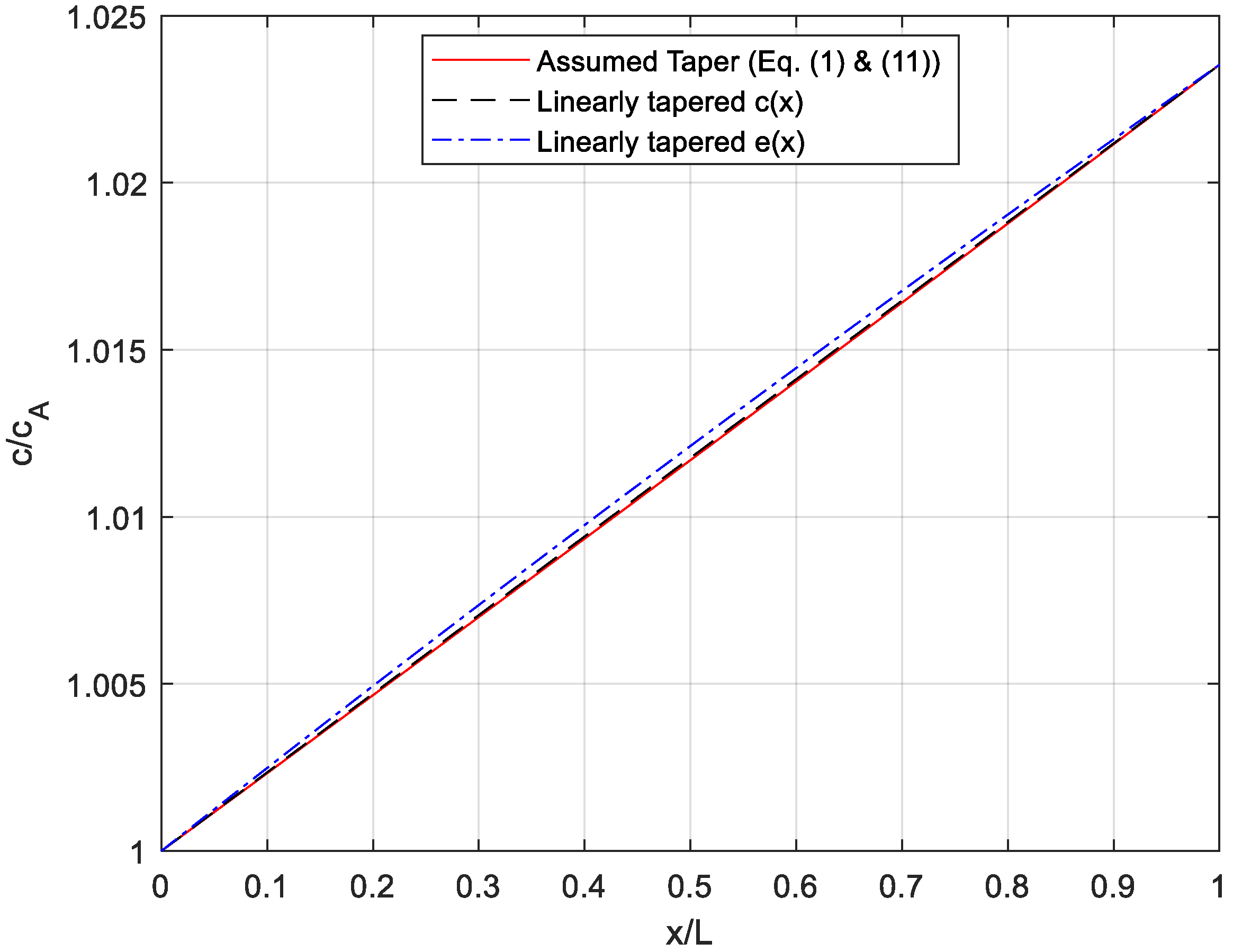
We now assume that the wave speed’s variation along the tube takes the form
where
and where and are the wave speeds at the inlet () and outlet (), respectively. As demonstrated in Figure 2, this nonlinear taper approximates a linear taper as long as the differences in are small relative to its absolute value. If this assumption is broken, the tube can be divided into a number of shorter segments.
For the nonlinear taper given above, the average velocity (as derived in Appendix A) is
This taper has the nice property of
which allows Equations (11) and (14) to be substituted into Equation (10) to give
If we define
then the ODE takes the form of
which has an analytical solution:
where and are the Bessel functions of the first and second kind, and and are constants of integration.
This can be substituted into Equation (5) to obtain the pressure solution
We can then apply open or closed boundary conditions to obtain the transmission matrix in the form
where and are the pressures at the inlet and outlet, and are the corresponding flow rates, and and are the characteristic impedances at the inlet and outlet:
The transmission matrix terms are
where
By applying the Wronskian, the denominator can be simplified to
The above equations are undefined at , but steady state physical requirements can be used to find the values. For continuity in flow between inlet and outlet, and zero pressure drop for zero flow:
For the proper steady state pressure drop
where is the Hagen–Poiseuille laminar resistance [22]. Note the relationship between and the dissipation number where is the lumped characteristic impedance, defined for a lossless line by
where is the lumped inductance and is the lumped capacitance [14,23]. For the tapered-wall tube defined in this paper, the dissipation number is
Numerical issues exist for combinations of high frequency and small tapers. This is due to the transmission matrix numerators being a small difference of large numbers. This problem can be mitigated by using quadruple precision floating point representations. An alternative is to use high-frequency approximations of the Bessel functions [24]. In the limit as
This allows for the following simplifications of the transmission matrix
We found that the approximation error of these equations is exceeded by the precision error of the original equations (for double precision floating point numbers) when the imaginary part of is greater than about 15.
3. Results
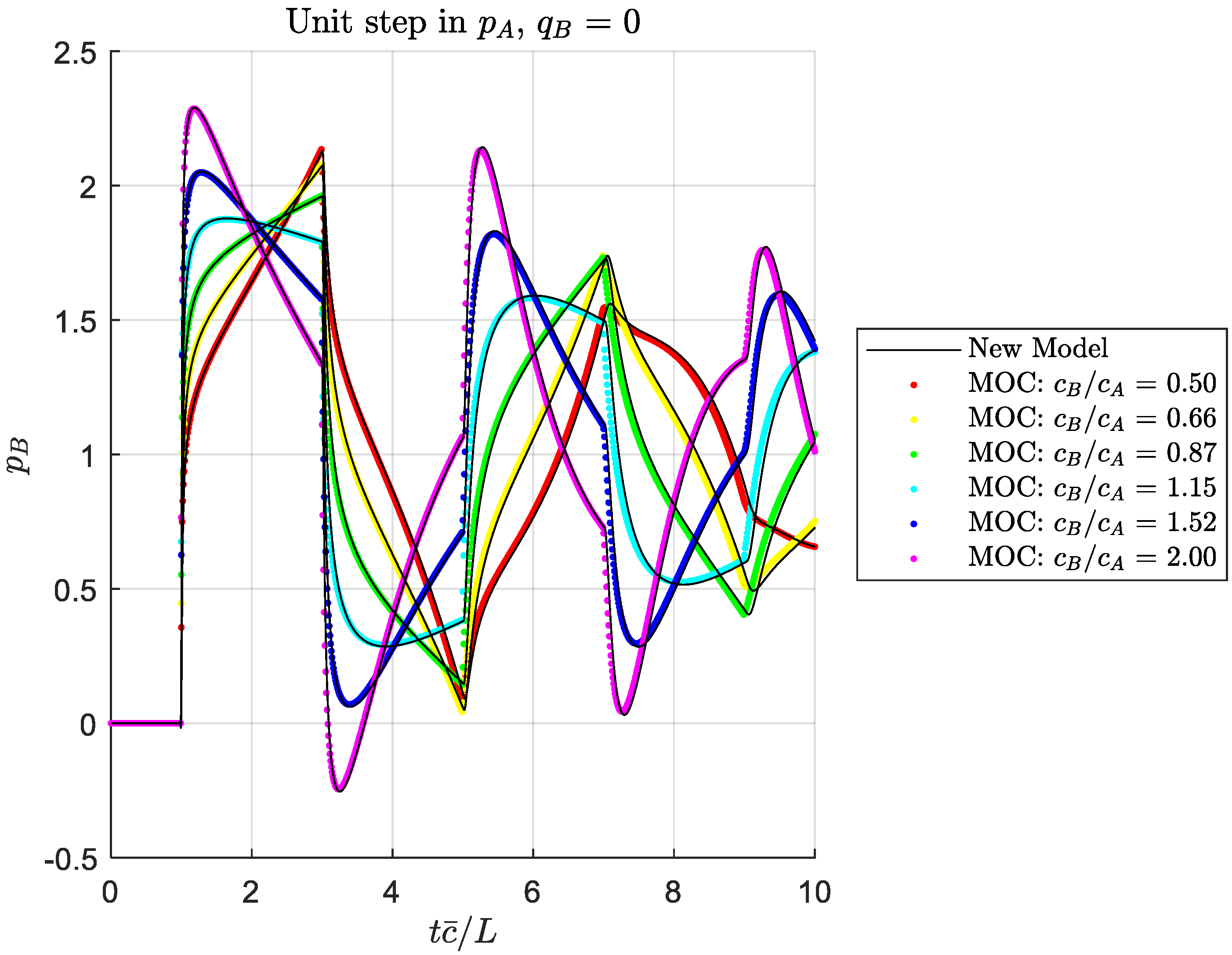
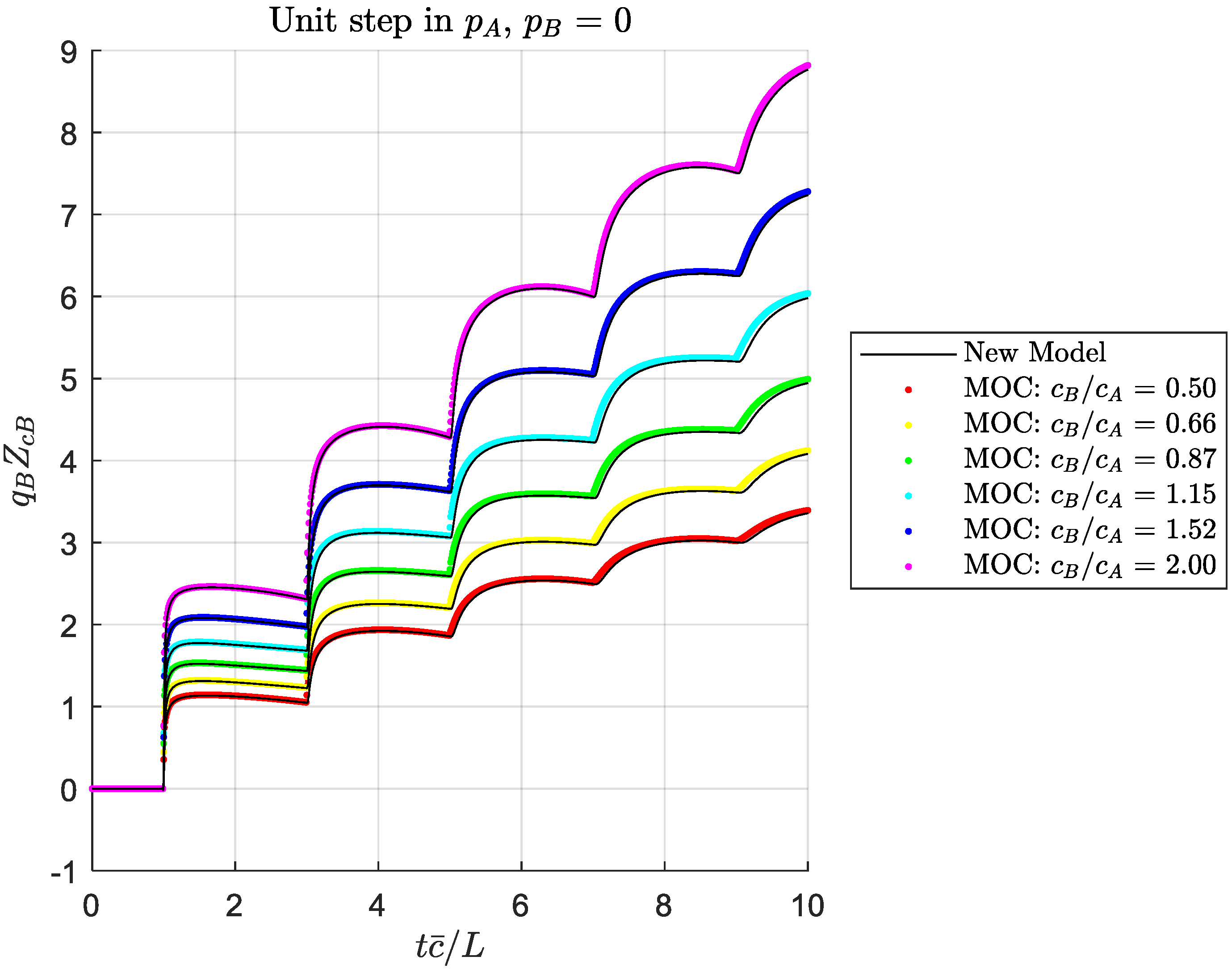
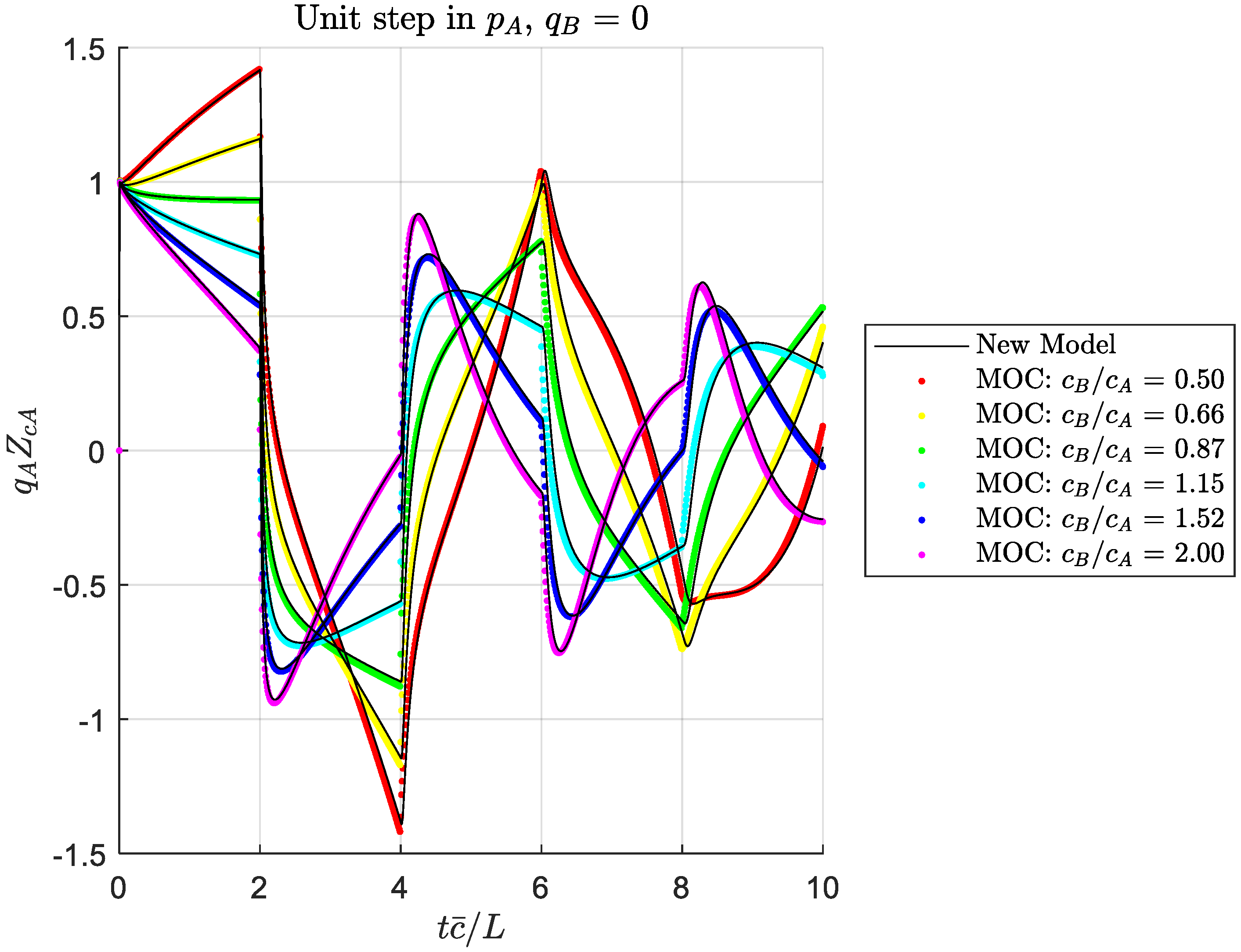
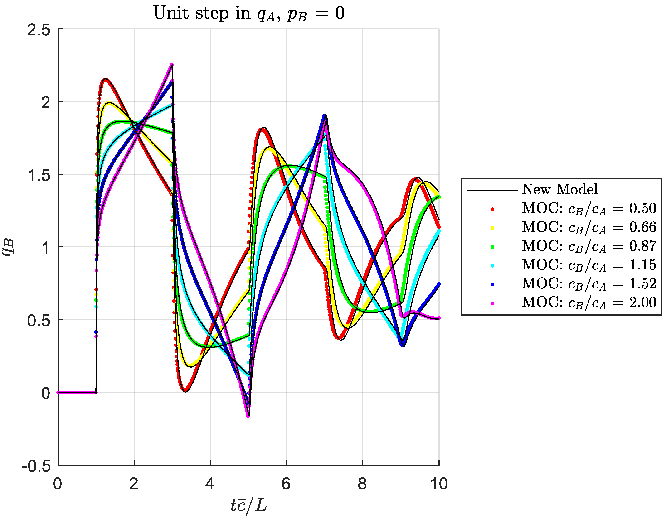
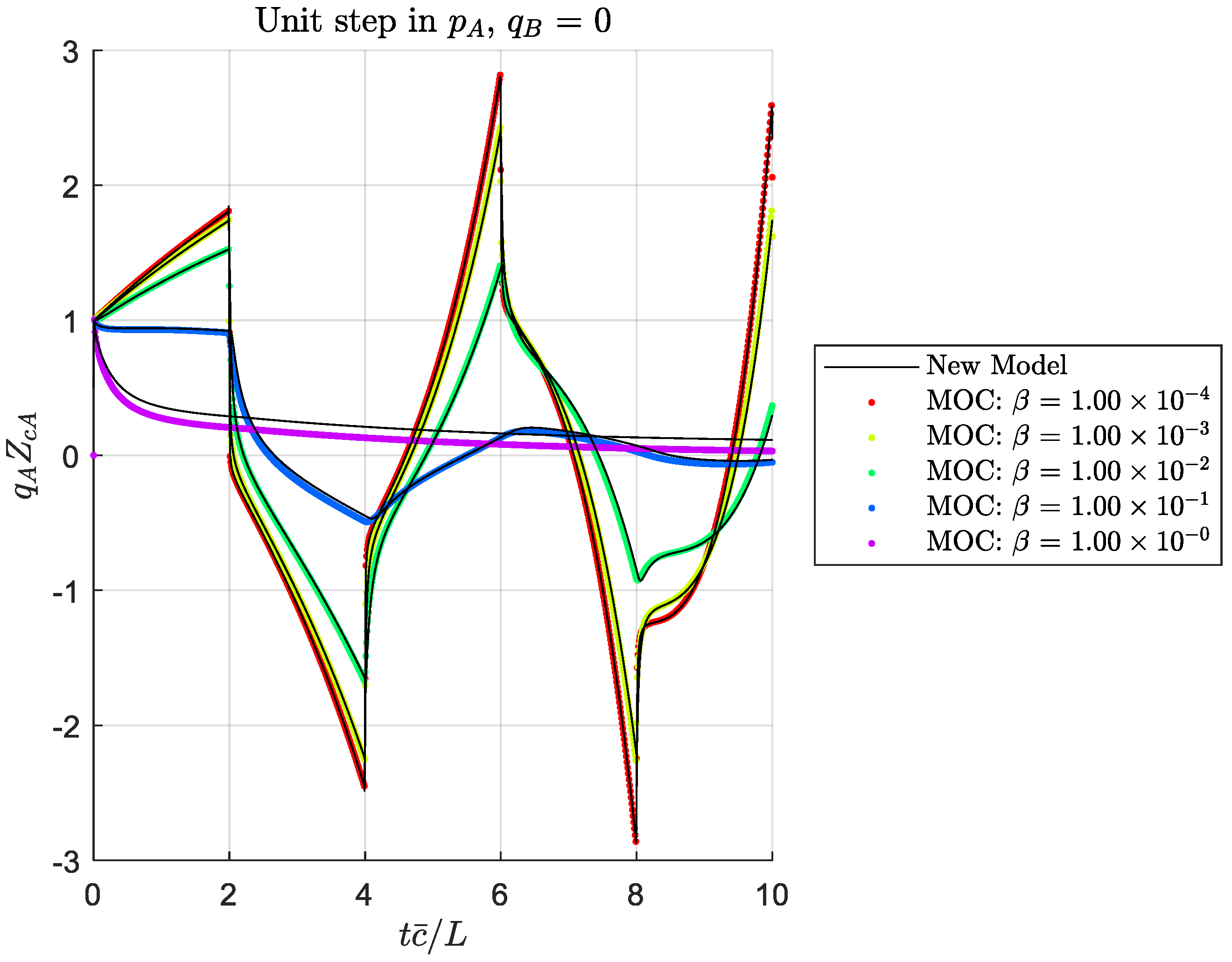
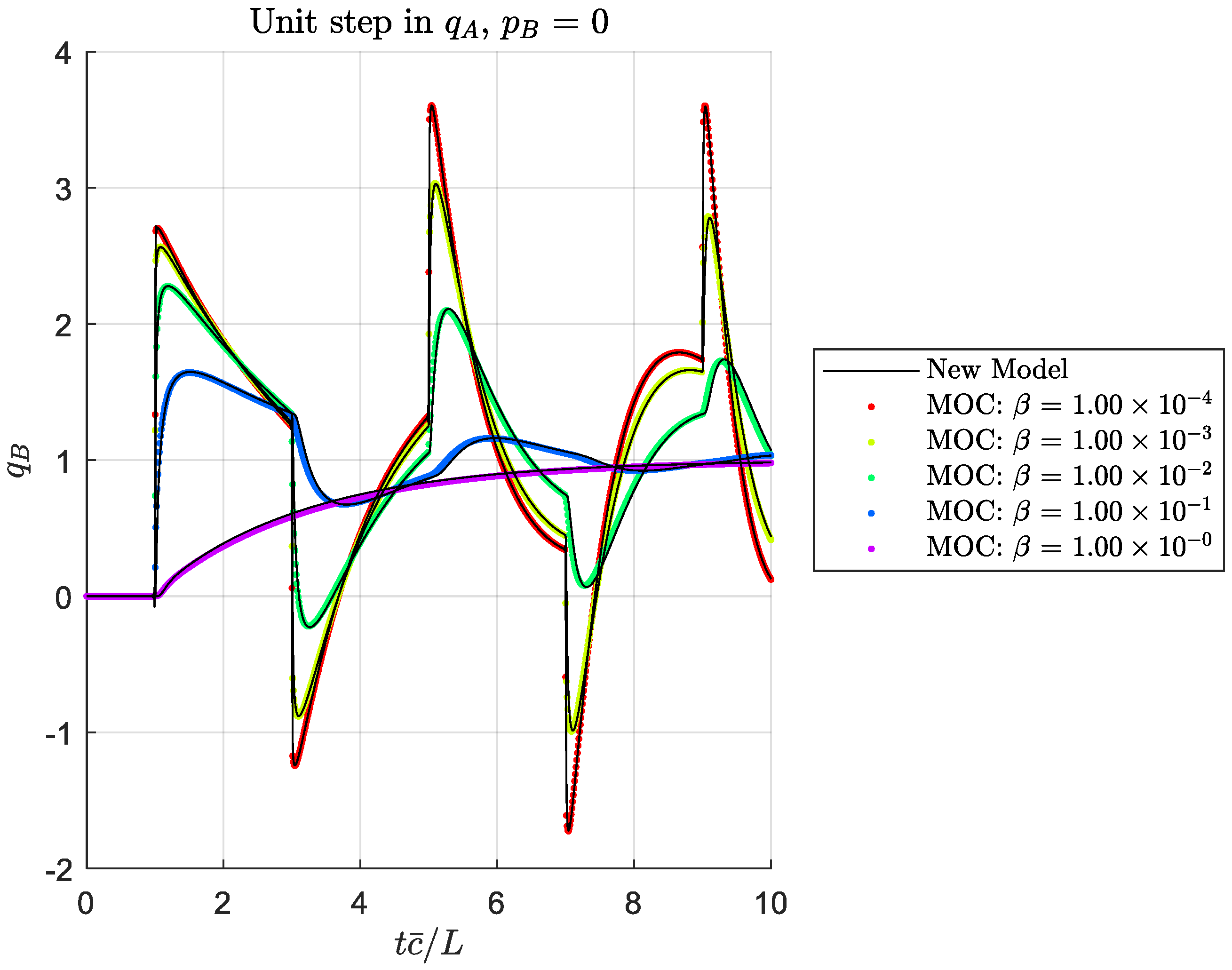
In order to verify the equations, we compared the calculated responses to a method of characteristics (MOC) solution. The MOC solution divides the tube into N = 100 segments, each with a constant wave velocity, and uses an approximate frequency-dependent friction model from [13]. Since the analytical solution presented in our paper does not include these approximations, one should not view the MOC solution as the “true” solution as much as a sanity check to ensure that no blunders were committed in our development.
Frequency-domain solutions were calculated using the transmission matrix terms for frequencies scaled so that 100 time points would be calculated in the time required for the wave to transit the length of the tube, and the solution would span 8000 such cycles. These 800,000 frequency points are not strictly required, but the calculation is fast and it was desirable to ensure the entire response was captured for low dissipation numbers. Considerably fewer frequency points would be required for more damped responses. The inverse Fourier transform was used to calculate the time-domain response from the frequency-domain response.
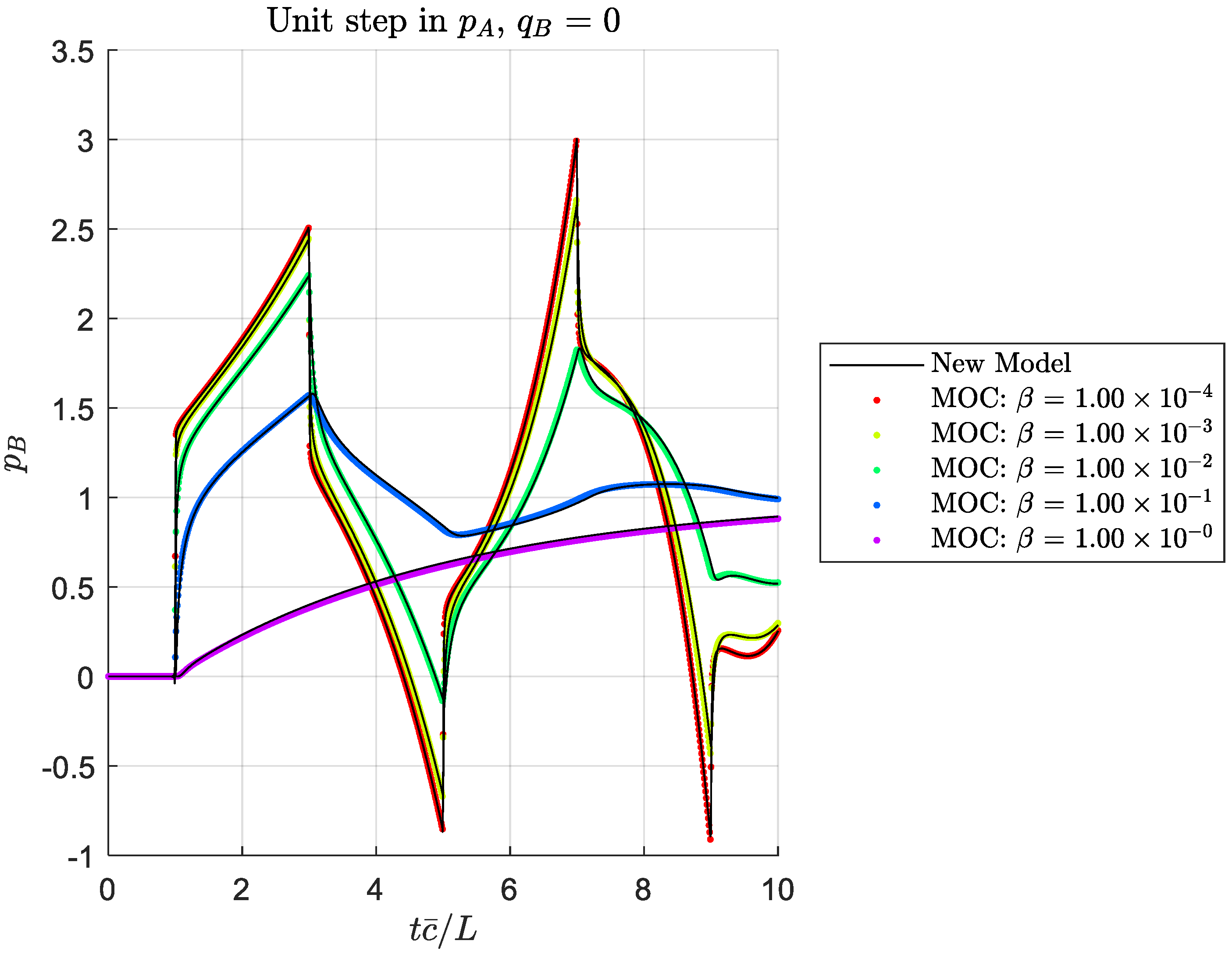
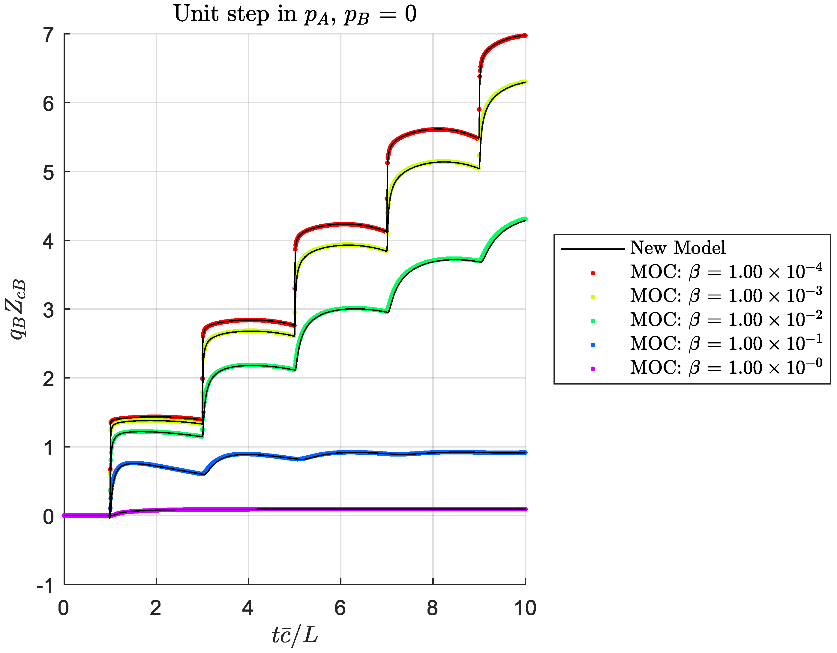
Figure 3, Figure 4, Figure 5, Figure 6, Figure 7, Figure 8, Figure 9 and Figure 10 show solutions for four boundary condition situations, involving all four of the transmission matrix terms. Figure 3, Figure 4, Figure 5 and Figure 6 show the effect of varying the outlet wave speed while holding other parameters constant (which would result in for . The solutions agree well, within the expected accuracy of the MOC solution. Figure 7, Figure 8, Figure 9 and Figure 10 show the same boundary conditions, but now holding constant and varying the viscosity to show a range of dissipation numbers (refer to Equation (37)). Again, the solutions agree well across the range of responses. At this point, we have not identified bounds for the applicability of our solution method, but we expect it should be suitable for all practical situations where the assumptions are satisfied.
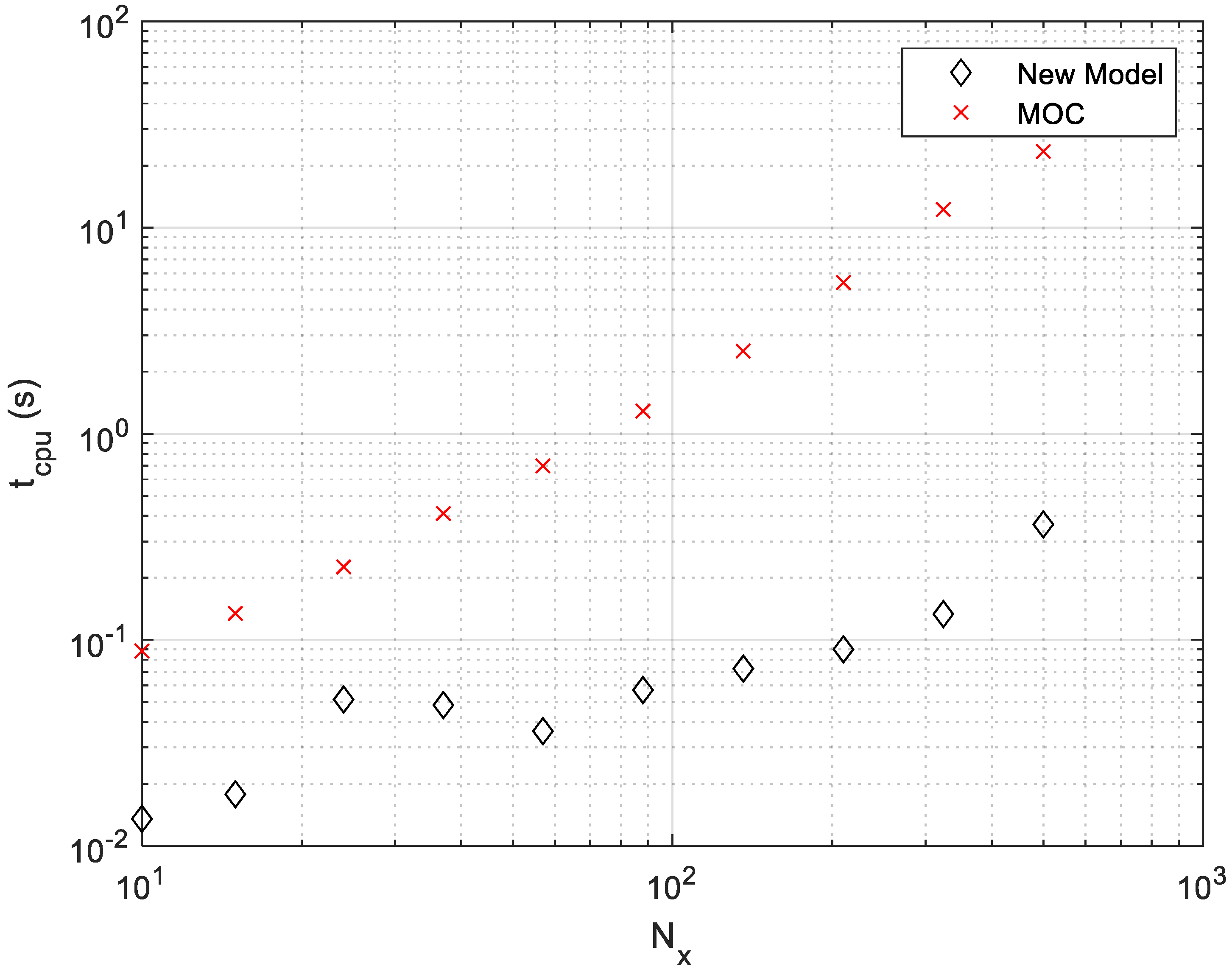
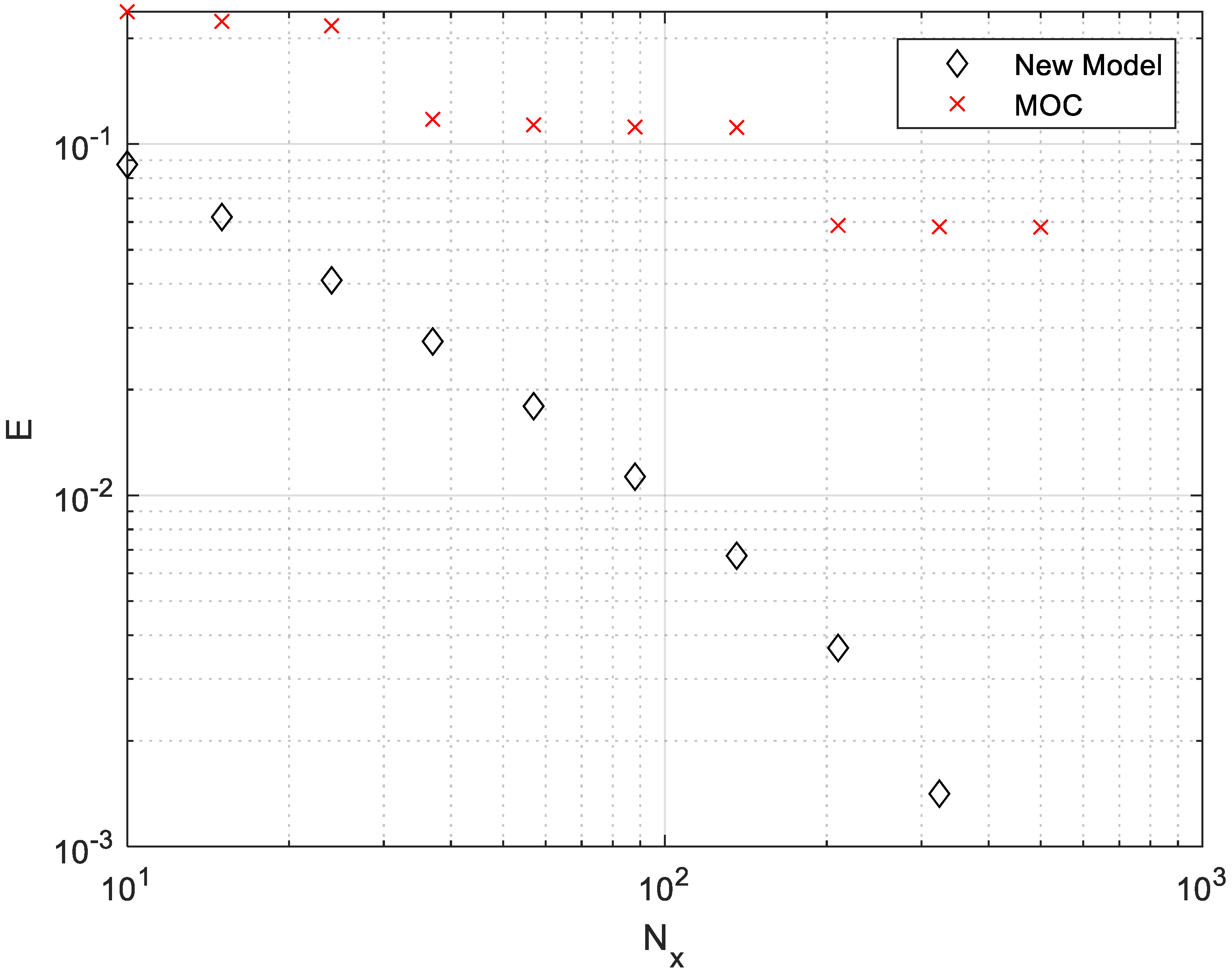
In order to provide a sense of the relative computational cost for the new frequency domain method, responses were calculated for the case of and while varying the number of frequency points in the solution. The method of characteristics solution was then calculated, with the grid selected to give results at the same time resolution. The computation time was recorded for each calculation, as implemented in MATLAB 2019b and run on a desktop computer with a i7-8700 processor with 32 GB RAM. In each case, the solution was calculated to an end time of four times the response’s settling time (defined as the point where transients reduce to 1% of the maximum value). The relative root mean squared error between the calculated response, and the highest resolution frequency-domain method response calculated, , normalized by the standard deviation, was calculated as
where an overbar designates the mean [25].
Figure 11 and Figure 12 shows the resultant calculation time and error as more terms are used in the solution. As expected, as the resolution is increased, the computation time and accuracy increase for both methods. However, for a given resolution, the new method is both faster (by around an order of magnitude) and more accurate. While the presented results are for a specific problem, we observed similar results across a wide range of dissipation numbers and taper ratios. It should be noted that neither the MOC solution nor the new frequency domain solution code was extensively optimized for speed, so these results should be viewed as a preliminary indication of relative computational speed.
One downside of the new method is that sufficient frequency points must be selected so that the transients have died out by the end of the corresponding time-domain response. Otherwise, the periodic nature of the Fourier transform will cause the response beyond the calculated end time to be added to the start of the response. If only the very beginning of a long response is of interest, the MOC method can be faster, as the computation can be halted early, while the new frequency-domain method must be fully calculated.
4. Summary and Conclusions
This paper presents an analytical solution for pressure and flow dynamics for laminar liquid flow within a tube, where the wave speed varies along the tube length in response to a change in compliance. This describes the situation of a tube with a flexible pipe wall where the wall thickness varies along the tube length but may also be applicable in other situations where the wave speed varies.
We have identified a numerical issue with standard double-precision floating point calculations and recommend two methods of mitigating these effects.
This paper also presents a comparison of the new method to a method of characteristics solution which agree well over a range of taper ratios and dissipation numbers, leading to confidence in the solution. A preliminary comparison of the calculation time and accuracy as the number of terms in the solution are varied is presented, which indicates that the new method is at least as accurate and much faster than the MOC solution.
Future work includes a more rigorous evaluation of the range of applicability of this new solution method, in terms of dissipation number and taper ratio, as well as an analysis of the number of frequency terms required for acceptable accuracy.
Author Contributions
Conceptualization, T.W. and E.E.; methodology, T.W.; resources, T.W.; writing T.W. and E.E. Both authors have read and agreed to the published version of the manuscript.
Funding
This research and APC were funded by NSERC and Mosaic Potash.
Institutional Review Board Statement
Not applicable.
Informed Consent Statement
Not applicable.
Data Availability Statement
Not applicable.
Acknowledgments
We would like to acknowledge Mathematics Stack Exchange user Paul Enta for assistance simplifying the Bessel functions.
Conflicts of Interest
The authors declare no conflict of interest.
Appendix A
This appendix derives the average velocity for a wave whose velocity is defined by
from to where
The position of a wave front that starts at at is given by the ODE
whose solution is
Therefore, the wave front arrives at at time
and, after some algebraic manipulation, the average velocity is
References
- Lowe, M.J.; Cawley, P. Long Range Guided Wave Inspection Usage—Current Commercial Capabilities and Research Directions; Department of Mechanical Engineering, Imperial College London: London, UK, 2006; pp. 1–40. [Google Scholar]
- Tennyson, R.C.; Morison, W.D.; Miesner, T. Pipeline Integrity Assessment Using Fiber Optic Sensors. In Pipelines 2005: Optimizing Pipeline Design, Operations and Maintenance in Today’s Economy, Proceedings of the ASCE Pipeline Division Specialty Conference (Pipelines 2005), Houston, TX, USA, 21–24 August 2005; American Society of Civil Engineers: Reston, VA, USA, 2005; pp. 803–817. [Google Scholar]
- Kishawy, H.A.; Gabbar, H.A. Review of pipeline integrity management practices. Int. J. Press. Vessel. Pip. 2010, 87, 373–380. [Google Scholar] [CrossRef]
- Ghidaoui, M.S.; Zhao, M.; McInnis, D.A.; Axworthy, D.H. A Review of Water Hammer Theory and Practice. Appl. Mech. Rev. 2005, 58, 49–76. [Google Scholar] [CrossRef]
- Montgolfier, J.-M. Note sur le bélier hydraulique: Et sur la maniere d’en calculer les effets. J. Mines 1803, 13, 42–51. [Google Scholar]
- Whitehurst, J. Account of a machine for raising water, executed at Oulton, in Cheshire, in 1772. In a letter from Mr. John Whitehurst to Dr. Franklin. Philos. Trans. (1683–1775) 1775, 65, 277–279. [Google Scholar]
- Young, B.W. Design of Hydraulic Ram Pump Systems. Proc. Inst. Mech. Eng. Part A J. Power Energy 1995, 209, 313–322. [Google Scholar] [CrossRef]
- Pan, M.; Johnston, N.; Robertson, J.; Plummer, A.; Hillis, A.; Yang, H. Experimental Investigation of a Switched Inertance Hydraulic System With a High-Speed Rotary Valve. J. Dyn. Syst. Meas. Control. 2015, 137, 121003. [Google Scholar] [CrossRef]
- Yudell, A.C.; Van de Ven, J.D. Soft switching in switched inertance hydraulic circuits. Fluid Power Sys. Tech. 2016, 50060, V001T01A040. [Google Scholar]
- Yuan, C.; Pan, M.; Plummer, A. A Review of Switched Inertance Hydraulic Converter Technology. BATH/ASME 2018 Symp. Fluid Power Motion Control 2018, 51968, V001T01A013. [Google Scholar] [CrossRef]
- Wiens, T.K. Analysis and Mitigation of Valve Switching Losses in Switched Inertance Converters. ASME/BATH 2015 Symp. Fluid Power Motion Control 2015. [Google Scholar] [CrossRef]
- Johnston, N.; Pan, M.; Kudzma, S.; Wang, P. Use of Pipeline Wave Propagation Model for Measuring Unsteady Flow Rate. J. Fluids Eng. 2014, 136, 031203. [Google Scholar] [CrossRef]
- Johnston, D.N. Efficient methods for numerical modelling of laminar friction in fluid lines. J. Dyn. Syst. Meas. Control Trans. ASME 2006, 128, 829–834. [Google Scholar] [CrossRef]
- Wiens, T.; Der Buhs, J.V.; Der Buhs, J.W.V. Transmission Line Modeling of Laminar Liquid Wave Propagation in Tapered Tubes. J. Fluids Eng. 2019, 141, 101103. [Google Scholar] [CrossRef]
- Krus, P.; Weddfelt, K.; Palmberg, J.-O. Fast Pipeline Models for Simulation of Hydraulic Systems. J. Dyn. Syst. Meas. Control. 1994, 116, 132–136. [Google Scholar] [CrossRef]
- Muto, T.; Kinoshita, Y.; Yoneda, R. Dynamic Response of Tapered Fluid Lines: 1st Report, Transfer Matrix and Frequency Response. Bull. JSME 1981, 24, 809–815. [Google Scholar] [CrossRef] [Green Version]
- Tahmeen, M.; Muto, T.; Yamada, H. Simulation of Dynamic Responses of Tapered Fluid Lines. JSME Int. J. Ser. B 2001, 44, 247–254. [Google Scholar] [CrossRef] [Green Version]
- D’Souza, A.F.; Oldenburger, R. Dynamic Response of Fluid Lines. J. Basic Eng. 1964, 86, 589–598. [Google Scholar] [CrossRef]
- Zielke, W. Frequency-Dependent Friction in Transient Pipe Flow. J. Basic Eng. 1968, 90, 109–115. [Google Scholar] [CrossRef]
- Johnston, D.N. Numerical modelling of unsteady turbulent flow in smooth-walled pipes. Proc. Inst. Mech. Eng. Part C: J. Mech. Eng. Sci. 2011, 225, 1601–1613. [Google Scholar] [CrossRef] [Green Version]
- Goodson, R.E.; Leonard, R.G. A Survey of Modeling Techniques for Fluid Line Transients. J. Basic Eng. 1972, 94, 474–482. [Google Scholar] [CrossRef]
- Sutera, S.P.; Skalak, R. The history of Poiseuille’s law. Annu. Rev. Fluid Mech. 1993, 25, 1–20. [Google Scholar] [CrossRef]
- Williams, T. The Circuit Designer’s Companion; Elsevier: Amsterdam, The Netherlands, 2004. [Google Scholar]
- Olver, F.W.J.; Olde Daalhuis, A.B.; Lozier, D.W.; Schneider, B.I.; Boisvert, R.F.; Clark, C.W.; Miller, B.R.; Saunders, B.V.; Cohl, H.S.; McClain, M.A. (Eds.) NIST Digital Library of Mathematical Functions. Available online: https://dlmf.nist.gov/ (accessed on 22 April 2021).
- Shcherbakov, M.V.; Brebels, A.; Shcherbakova, N.L.; Tyukov, A.P.; Janovsky, T.A.; Kamaev, V.A.E. A survey of forecast error measures. World Appl. Sci. J. 2013, 24, 171–176. [Google Scholar]
Figure 1.
Flow through a circular tube with varying wall thickness and, consequently, varying wave propagation velocity. (Wall thickness and diameter are exaggerated.)
Figure 1.
Flow through a circular tube with varying wall thickness and, consequently, varying wave propagation velocity. (Wall thickness and diameter are exaggerated.)

Figure 2.
The wave speed profile assumed in Equation (11) results in a wave speed that approximates both the case where the wave speed varies linearly and the case where the tube’s wall thickness varies linearly, as long as the variation in wave speed is small relative to its absolute value. (This example was calculated for E = 200 GPa and K = 1 GPa).

Figure 3.
Outlet pressure response to a unit step in inlet pressure, for a closed exit, showing effect of taper ratio.
Figure 3.
Outlet pressure response to a unit step in inlet pressure, for a closed exit, showing effect of taper ratio.

Figure 4.
Outlet flow response to a unit step in inlet pressure, for an open exit, showing effect of taper ratio.
Figure 4.
Outlet flow response to a unit step in inlet pressure, for an open exit, showing effect of taper ratio.

Figure 5.
Inlet flow response to a unit step in inlet pressure, for a closed exit, showing effect of taper ratio.
Figure 5.
Inlet flow response to a unit step in inlet pressure, for a closed exit, showing effect of taper ratio.

Figure 6.
Outlet flow response to a unit step in inlet flow, for an open exit, showing effect of taper ratio.
Figure 6.
Outlet flow response to a unit step in inlet flow, for an open exit, showing effect of taper ratio.

Figure 7.
Outlet pressure response to a unit step in inlet pressure for a closed exit, showing the effect of dissipation number (for ).
Figure 7.
Outlet pressure response to a unit step in inlet pressure for a closed exit, showing the effect of dissipation number (for ).

Figure 8.
Outlet flow response to a unit step in inlet pressure for an open exit, showing the effect of dissipation number (for ).
Figure 8.
Outlet flow response to a unit step in inlet pressure for an open exit, showing the effect of dissipation number (for ).

Figure 9.
Inlet flow response to a unit step in inlet pressure for a closed exit, showing the effect of dissipation number (for ).
Figure 9.
Inlet flow response to a unit step in inlet pressure for a closed exit, showing the effect of dissipation number (for ).

Figure 10.
Outlet flow response to a unit step in inlet flow for an open exit, showing the effect of dissipation number (for ).
Figure 10.
Outlet flow response to a unit step in inlet flow for an open exit, showing the effect of dissipation number (for ).

Figure 11.
Computation time required to calculate a sample solution, as the time resolution is varied. For the MOC case, corresponds to the number of spatial grid points. For the frequency-domain case, the frequency points were selected to give the same time resolution as the MOC case.
Figure 11.
Computation time required to calculate a sample solution, as the time resolution is varied. For the MOC case, corresponds to the number of spatial grid points. For the frequency-domain case, the frequency points were selected to give the same time resolution as the MOC case.

Figure 12.
Normalized error for the same data as Figure 11.
Figure 12.
Normalized error for the same data as Figure 11.

Publisher’s Note: MDPI stays neutral with regard to jurisdictional claims in published maps and institutional affiliations. |
© 2021 by the authors. Licensee MDPI, Basel, Switzerland. This article is an open access article distributed under the terms and conditions of the Creative Commons Attribution (CC BY) license (https://creativecommons.org/licenses/by/4.0/).
Share and Cite
MDPI and ACS Style
Wiens, T.; Etminan, E. An Analytical Solution for Unsteady Laminar Flow in Tubes with a Tapered Wall Thickness. Fluids 2021, 6, 170. https://0-doi-org.brum.beds.ac.uk/10.3390/fluids6050170
AMA Style
Wiens T, Etminan E. An Analytical Solution for Unsteady Laminar Flow in Tubes with a Tapered Wall Thickness. Fluids. 2021; 6(5):170. https://0-doi-org.brum.beds.ac.uk/10.3390/fluids6050170
Chicago/Turabian StyleWiens, Travis, and Elnaz Etminan. 2021. "An Analytical Solution for Unsteady Laminar Flow in Tubes with a Tapered Wall Thickness" Fluids 6, no. 5: 170. https://0-doi-org.brum.beds.ac.uk/10.3390/fluids6050170