
Experiments and Modeling of a Compliant Wall Response to a Turbulent Boundary Layer with Dynamic Roughness Forcing


Graduate Aerospace Laboratories, California Institute of Technology, 1200 East California Boulevard, Pasadena, CA 91125, USA
*
Author to whom correspondence should be addressed.
Fluids 2021, 6(5), 173; https://0-doi-org.brum.beds.ac.uk/10.3390/fluids6050173
Submission received: 30 March 2021
/
Revised: 16 April 2021
/
Accepted: 20 April 2021
/
Published: 26 April 2021
(This article belongs to the Special Issue Turbulent Flows at Solid and Free Surface Boundaries in Memory of William W. Willmarth)
Abstract
:The response of a compliant surface in a turbulent boundary layer forced by a dynamic roughness is studied using experiments and resolvent analysis. Water tunnel experiments are carried out at a friction Reynolds number of , with flow and surface measurements taken with 2D particle image velocimetry (PIV) and stereo digital image correlation (DIC). The narrow band dynamic roughness forcing enables analysis of the flow and surface responses coherent with the forcing frequency, and the corresponding Fourier modes are extracted and compared with resolvent modes. The resolvent modes capture the structures of the experimental Fourier modes and the resolvent with eddy viscosity improves the matching. The comparison of smooth and compliant wall resolvent modes predicts a virtual wall feature in the wall normal velocity of the compliant wall case. The virtual wall is revealed in experimental data using a conditional average informed by the resolvent prediction. Finally, the change to the resolvent modes due to the influence of wall compliance is studied by modeling the compliant wall boundary condition as a deterministic forcing to the smooth wall resolvent framework.
1. Introduction
One of the long-standing engineering goals for research in wall-bounded turbulent flows is to develop design capabilities for flow control mechanisms. Designing such control schemes within the broad field of possible applications and strategies [1] is difficult not only due to the essential complexity of actuator–flow interaction, but also the often vast operational parameter space associated with actuation design. Compliant surfaces embody both of these challenges, presenting a coupled fluid-structural problem and nearly limitless regime of surface material properties. However, the potential benefits of these passive controllers has spurred a field of research that remains active today [2].
A number of experimental studies have found promising results. Lee et al. [3] conducted a water tunnel experiment of a turbulent boundary layer with a single-layer viscoelastic surface and observed a modification to the low-speed streaks associated with the near-wall cycle accompanied by a reduction in the streamwise turbulence intensity and Reynolds shear stress. In a similar experiment, Choi et al. [4] reported drag reduction on a slender body of revolution as high as 7%. Wang et al. [5] studied the wall deformation and flow response over a compliant wall for a range of material properties and identified the associated changes to the mean velocity and turbulence profiles. Tempering some of the optimistic experimental findings are more recent Direct Numerical Simulation (DNS) studies. Xu et al. [6] simulated a turbulent channel flow with a compliant wall modelled as a spring-supported plate and found little change to the turbulent skin friction. Fukagata et al. [7] considered an anisotropic compliant wall and observed an 8% maximum drag reduction, but this effect diminished as the computational domain was increased. In simulations of turbulent channel flow over a viscous hyper-elastic wall, Rosti and Brandt [8] described changes to the near-wall flow structure associated with non-zero vertical velocities at the moving wall.
As experimental and computational studies of compliant surfaces are costly and time-consuming, there is a need for accurate reduced-order models to provide insight and reduce the otherwise intractable parameter space. The recent work of Benschop et al. [9] employed a one-way model to predict the wall-normal surface deformation of a compliant coating in a turbulent flow. The model was restricted to spanwise-constant, streamwise-travelling deformations and required as input the turbulent stress spectra, convection velocity, and frequency-dependent surface properties. The authors performed an extensive parametric study, investigating the effects of the density, stiffness, thickness, viscoelasticity, and compressibility of the surface on the wall-normal deformation. In a separate modelling effort, Luhar et al. [10] extended the resolvent formulation of McKeon and Sharma [11] to consider the influence of a compliant-wall on a turbulent flow, as described in detail in subsequent Section 2.2. See [12,13] for recent reviews of the efficacy of resolvent-based approaches for modeling wall turbulence. The resolvent-based model is derived by recasting the Fourier-transformed Navier–Stokes equations (NSEs) into an input-output form, where the nonlinear term is explicitly retained as an endogenous forcing to the linear dynamics. The most amplified response modes of the resolvent operator are then identified through a singular-value decomposition (SVD). Luhar et al. [10] modified the rigid-wall boundary condition to account for wall compliance. The model only required the mean velocity profile, a wall compliance parameter, and a wavenumber vector as input, and was used to search for optimal wall (material) properties to reduce the amplification of physically relevant flow structures. The results were found to compare favorably with trends elucidated in DNS studies.
This work seeks to compare and extend the predictions of the compliant wall resolvent analysis [10] to experiments of a turbulent boundary layer with an elastic compliant wall, and simultaneously to use the resolvent predictions as a lens to inform the analysis of the experimental data. Further, we model the effect of the boundary condition as an extra forcing in the resolvent framework, with a view to simplifying future numerical studies. The experiments utilize a two-dimensional (spanwise constant) dynamic roughness forcing, which forces a spectrally narrow synthetic flow mode, which in turn interacts with the surface. This allows for a direct mode comparison between the model prediction and the experimental data. This manuscript serves as the culmination of a series of manuscripts pertaining to the different stages of this experimental and modeling study: Huynh and McKeon [14] documented the influence of the dynamic roughness studied here on the flow over a rigid wall, while Huynh and McKeon [15] documented the experimental configuration to identify the compliant wall response to that synthetic forcing input. The present work constitutes the first experimental demonstration of the efficacy of resolvent analysis in modeling the response of a compliant wall beneath a turbulent boundary layer. In what follows, we outline the compliant wall resolvent framework, describe and summarize results from the experiment, discuss the comparison between the resolvent and experimental modes and develop the boundary condition as forcing approach.
2. Materials and Methods
2.1. Experimental Setup
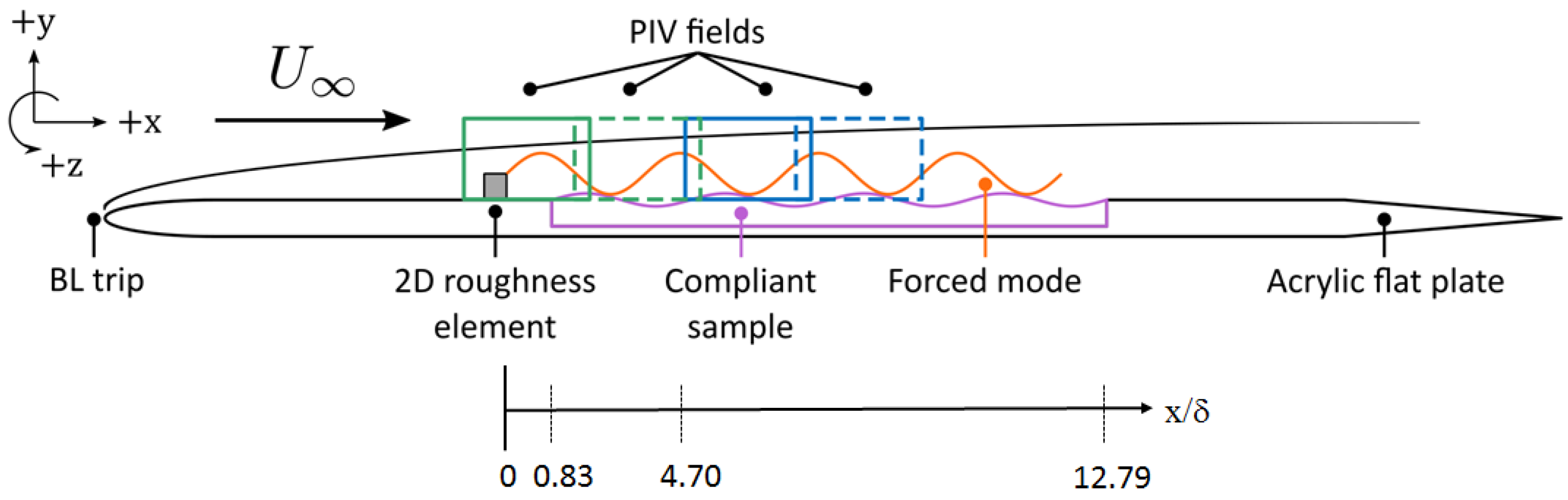
A full description of the experimental setup can be found in Huynh and McKeon [14] and Huynh and McKeon [15], which describe the response of the rigid wall turbulent boundary layer and compliant wall to dynamic roughness forcing, respectively. A brief summary is provided here. The experiments were performed in the NOAH water tunnel at Caltech. Figure 1 shows an illustration of the experiment. The flow was tripped at the leading edge of the acrylic plate to promote a turbulent boundary layer. A thin, spanwise-constant aluminum rib served as the two-dimensional dynamic roughness element, located 63 cm downstream of the leading edge (taken to be ), actuated perpendicularly to the plate by a Bose ElectroForce 200 N motor. The control configuration used a rigid wall downstream of the dynamic roughness. Then a compliant surface (gelatin) was embedded into the acrylic plate 25.4 mm downstream of the roughness element (Figure 2). Measurements were made of the flow velocity using 2D particle image velocimetry (PIV) in the plane, and the surface deformations using stereo digital image correlation (DIC) in the plane coincident with the surface. The streamwise and wall-normal velocities are denoted u and v, and the streamwise, wall-normal, and spanwise surface displacements are , , and , respectively. Both PIV and DIC were acquired using LaVision’s DaVis software. The properties of the canonical flow are summarized in Table 1, acquired from PIV at the roughness location. The friction velocity, , where is the wall shear stress, was estimated using the Clauser chart method, and the viscous length scale, , and friction Reynolds number, , were calculated accordingly.
The dynamic roughness was actuated sinusoidally, going from flush to the wall to full extension. This type of forcing has been shown to generate a synthetic, travelling-wave type flow structure that is well-modeled by the form for a 2D (spanwise constant) roughness, where is the angular forcing frequency and is the dominant streamwise wavenumber of the perturbation [14,16,17,18]. The actuation frequency and amplitude conditions considered are given in Table 2. The amplitudes were selected to be similar to those of Duvvuri and McKeon [17], while the frequencies were chosen to be significantly higher (in a dimensionless sense) to generate shorter synthetic flow structures, enabling a more spatially-resolved investigation. Most of the results discussed in this paper pertain to actuation condition iii. Both the PIV and DIC measurements were phase-locked to the roughness motion to enable a phase-averaged analysis. The camera frame rates were set to 20 times the actuation frequency for sufficient phase resolution. The discrete phase index, , will be used for reference, where corresponds to the roughness element flush to the wall.
Gelatin was selected as the material for this study due to its low cost, high deformability, and nearly linearly elastic behavior [19]. Because this study sought to compare results with modelled predictions, it was more important to have a measurable surface response to the roughness-forced synthetic mode rather than to achieve a particular performance metric. The gelatin was fabricated using a 1:25 gelatin–water ratio and molded directly into a section of the flat plate. Through simple compression tests, the Young’s modulus of the gelatin was measured to be kPa, and by assuming a Poisson’s ratio of 0.5 as is often used for gelatin [20], the shear modulus and shear wave speed were estimated to be kPa and m/s, respectively. This corresponds to an extremely soft material, though the low freestream velocity ( m/s) relative to the shear wave speed meant that hydroelastic instabilities were not expected. As discussed in Huynh and McKeon (2020), the Rayleigh, generalized Rayleigh, and Love wave speeds were also all calculated to be significantly larger than the freestream velocity, namely 1.15, 1.18, and 1.32 m/s, respectively.
For convenience, the rigid-wall and compliant wall studies will be referred to as ‘RW’ and ‘CW’, and the dynamic-roughness-forced and unforced studies as ‘DRF’ and ‘unforced’, respectively.
2.2. Resolvent Analysis for Compliant Walls
McKeon and Sharma [11] applied the resolvent framework as an approach to study problems in turbulent flow in a low-rank manner by investigating the preferentially amplified modes of the resolvent operator. Here, the formulation by Luhar et al. [10] will be considered, for a fully developed channel flow, with x, y, and z corresponding to the streamwise, wall-normal, and spanwise directions, walls at and , the channel half-height denoted h. All terms in the following methodology have been non-dimensionalized using h and . A Fourier decomposition is employed in the homogeneous directions, x, z, and t:
where is the Fourier wavenumber vector and is the corresponding Fourier coefficient.
The Navier–Stokes equations (NSEs) are written in primitive-variable form, with pressure explicitly retained to later solve for the boundary condition. The NSEs are then Fourier-transformed and written in an input-output form:
where and are the Fourier-transformed velocity and pressure fields and is the Fourier-transformed nonlinear term:
and represent the Fourier-transformed gradient and divergence operators, respectively. In this framework, the nonlinear term acts as an endogenous forcing to the velocity and pressure through the resolvent operator, , which depends on the linear component of the NSEs:
where is the Fourier-transformed Laplacian. Note that contains terms with the mean velocity, , which is assumed to be known a priori.
The problem is discretized in y using N Chebyshev collocation points, then the discrete resolvent operator is constructed, and a singular value decomposition (SVD) is performed:
where are the singular response modes (henceforth referred to as resolvent modes), are the (ordered) singular values, and are the singular forcing modes. Superscript * denotes a complex conjugate. Velocity and pressure can then be expressed as:
where indicates an inner product and are the weights formed by projecting the nonlinear forcing onto the singular forcing modes.
A rank-1 reduction may be invoked to give a first approximation to the resolvent operator using the first resolvent mode, singular value, and singular forcing mode:
This then allows the velocity and pressure to be approximated by:
with the additional assumption of broadband forcing, discussed in McKeon and Sharma [11]. It will be seen that the essential features of the flow response are contained in the rank-1 model. In what follows, the subscript ‘’ will be suppressed and will indicate the response component, i.e., , , and for the streamwise, wall-normal, and pressure resolvent modes.
More accurate approximations can be obtained by retaining a higher rank representation of the resolvent, or by including an eddy viscosity in the linearized equations as a partial model of the influence of the nonlinear interaction of all scales, e.g., ref. [21,22]. We investigate the latter approach here.
Following Reynolds and Hussain [23], an analytic approximation for the turbulent eddy viscosity is used
where is the total effective viscosity normalized by . The viscous terms in Equation (4) are then replaced by
The parameters and are chosen based on a least-squares fit to experimentally obtained mean velocity profiles at [21]. Note that with the inclusion of the eddy viscosity, the interpretation of the nonlinear forcing given in Equation (3) is also different.
The framework by Luhar et al. [10] models the effect of a compliant wall by modifying the otherwise rigid wall boundary condition. Compliance is considered by introducing a wall displacement term at the boundaries, , constrained to be in the wall-normal direction. Along the boundary, the no-slip and no-through flow conditions are applied. A Taylor’s expansion is performed about the undeformed wall location; these boundary conditions can be made for an arbitrarily large wall deformation by retaining higher-order terms in the expansion, at the cost of a more complex, nonlinear set of equations. Instead, following Luhar et al. [10], the deformations are assumed small and the boundary conditions are linearized to enable a more computationally tractable analysis. Given the small deformations observed in the DIC data, , this assumption is at least somewhat justified and will be considered when interpreting the results. Thus, the linearized, Fourier-transformed velocity boundary conditions can be written as:
Note that is required to balance a mean shear term introduced by the wall deformation, and that is related to the deformation by the no-through flow boundary condition. Furthermore, Equations (11) and (12) together require that has a phase lead with respect to at the wall.
The pressure boundary condition is determined by the dynamic coupling between pressure and the wall motion. Here, this coupling is modelled as a spring-mass-damper system [6], for which the wall pressure and wall deformation are connected by:
where , , and are the dimensionless mass, damping, and spring coefficients. These coefficients are defined as:
where the following are all plate properties with subscript ‘w’ for ‘wall’: is the density, the thickness, the damping coefficient, and the area-spring stiffness. Though not considered in this analysis, additional tension and stiffness coefficients, and , respectively, can be included to account for the effects of tension and flexural rigidity (stiffness) of the plate. This can be achieved by substituting a wavenumber-dependent effective spring coefficient, , for in Equation (14), defined as:
assuming equal tension in x and z. Definitions of and can be found in Xu et al. (2003) [6]. See also Luhar et al. (2016) [24].
A complex wall admittance term, Y, is defined that connects the pressure and the wall-normal velocity at the wall, and using Equations (12) and (14) is written as:
This complex admittance is used to account for the material properties of the wall. Thus, Equations (11)–(13) and (19) are used as the boundary conditions for the velocities and pressure at and , with the sign of Y flipped between the two walls due to centerline symmetry.
The MATLAB code for channel flow resolvent analysis with a compliant wall boundary condition [10] was used to generate the results discussed here. A study was also performed with a boundary layer configuration [16,25], with identical results near the wall and only slight differences in the outer part of the flow, as to be expected from considerations of near-wall universality and the influence of the semi-infinite boundary layer domain. A quasi-streamwise parallel assumption, or slow streamwise growth of the boundary layer of the field of view, is required to use a one-dimensional mean profile varying only in y. Given an approximate growth in boundary layer thickness over the entire compliant panel of ∼8% and the experimental uncertainties described below, this was deemed an acceptable simplification in light of the cost reduction associated with performing the SVD. While an experimental mean profile could have been used to account for the modification from the dynamic roughness, this would have required a choice of interpolation scheme and would have become difficult near the wall due to the inherent limitations of PIV. Therefore, the mean velocity profile is generated using the eddy viscosity model of Equation (9) for an uncontrolled mean flow, i.e., the same mean profile is used for both the rigid-wall and compliant wall resolvent modes, which is an additional simplification. Note that the mean velocity profile is an input to the resolvent model, which therefore cannot identify any net drag reduction or increase due to the presence of the compliant wall. However, changes in the response modes determined from the resolvent at individual scales due to the change in boundary condition can be interrogated. Further description is provided in Luhar et al. [10]. The grid resolution used was , and the friction Reynolds number of was used to match to experimental flow conditions. The code was executed on a single-core laptop and took about 0.5 s to compute one set of singular values and resolvent modes.
2.3. Compliant Wall as a Boundary Forcing
We now extend the analysis of [10] to provide an alternate model of the linearized boundary conditions for compliant wall resolvent analysis as an additional forcing term.
In general, any boundary condition of the form
where is any vector of constant coefficients, can be applied to the linear operator given in Equation (2) by substituting the rows corresponding to the boundary values of with and the same rows of with zeros. This form of boundary condition includes the no-slip boundary conditions and the linearized compliant wall boundary conditions described previously. With the properly applied boundary conditions, the resolvent operator can then be formed according to Equation (2), and its SVD can be computed. Using the orthonormal property of the singular vectors, Equation (5) can be rewritten as:
on the left hand side of the equation is the output of the system subjected to the input . For the case of a broadband forcing, the velocity and pressure Fourier modes can be approximated by as described in Equation (8), with describing the amplitude and describing the shape of the output. We now define a new, non-normalized response mode
which captures the output mode shape and energy together. Using the definition of , we arrive at
In what follows, only the rank-1 approximation will be considered, and the subscript ‘’ will again be suppressed.
The change of boundary conditions can be viewed as a perturbation of the rigid wall linear operator . We denote the linear operator with the compliant wall boundary condition as , its forcing mode as , its non-normalized response mode as , and the change in quantity denoted by . Additionally, we denote the rigid wall resolvent as , and the compliant wall resolvent as , with the difference . The perturbed linear operator and its forcing and reponse modes satisfy the perturbed form of Equation (23)
This equation can be rearranged into
The right-hand side terms describe the extra forcing needed to capture the change of response due to the compliant wall boundary conditions. The first term on the right, , involves the mass matrix and therefore has zero boundary values and non-zero values away from the boundary. The second term, , involves the perturbation matrix , and therefore is only non-zero at the boundaries; in other words, consists of delta functions at the wall.
, the total change in the response mode, can be split into two pieces, and , which correspond to the effect of and , and can be rewritten as
It should be noted that the form of the boundary conditions is not unique. For example, a no slip boundary condition can be written as , or equivalently written as (for ). As a result, the perturbation matrix and therefore are both non-unique. However, the change in response due to , denoted as in Equation (28) is the same regardless of the non-uniqueness of .
Equation (27) indicates that is the result of the change in forcing mode. From an optimization point of view, the first forcing mode is a unit energy mode that maximizes the energy of . Therefore, as the flow configuration changes, the forcing mode also changes to achieve this maximum. On the other hand, Equation (28) indicates that describes the change in response directly attributed to the change in boundary condition. For the compliant wall case studied here, induces non-zero boundary values in the streamwise and wall-normal directions as a result of the pressure at the wall that deforms the compliant surface.
In what follows, the structure of both contributions in Equation (26) to the change in response relative to the smooth wall case will be explored for the parameters corresponding to the experimental compliant wall in order to understand the origin of the change in the resolvent and experimental mode shapes.
3. Results
3.1. Flow Response and Flow-Wall Coupling
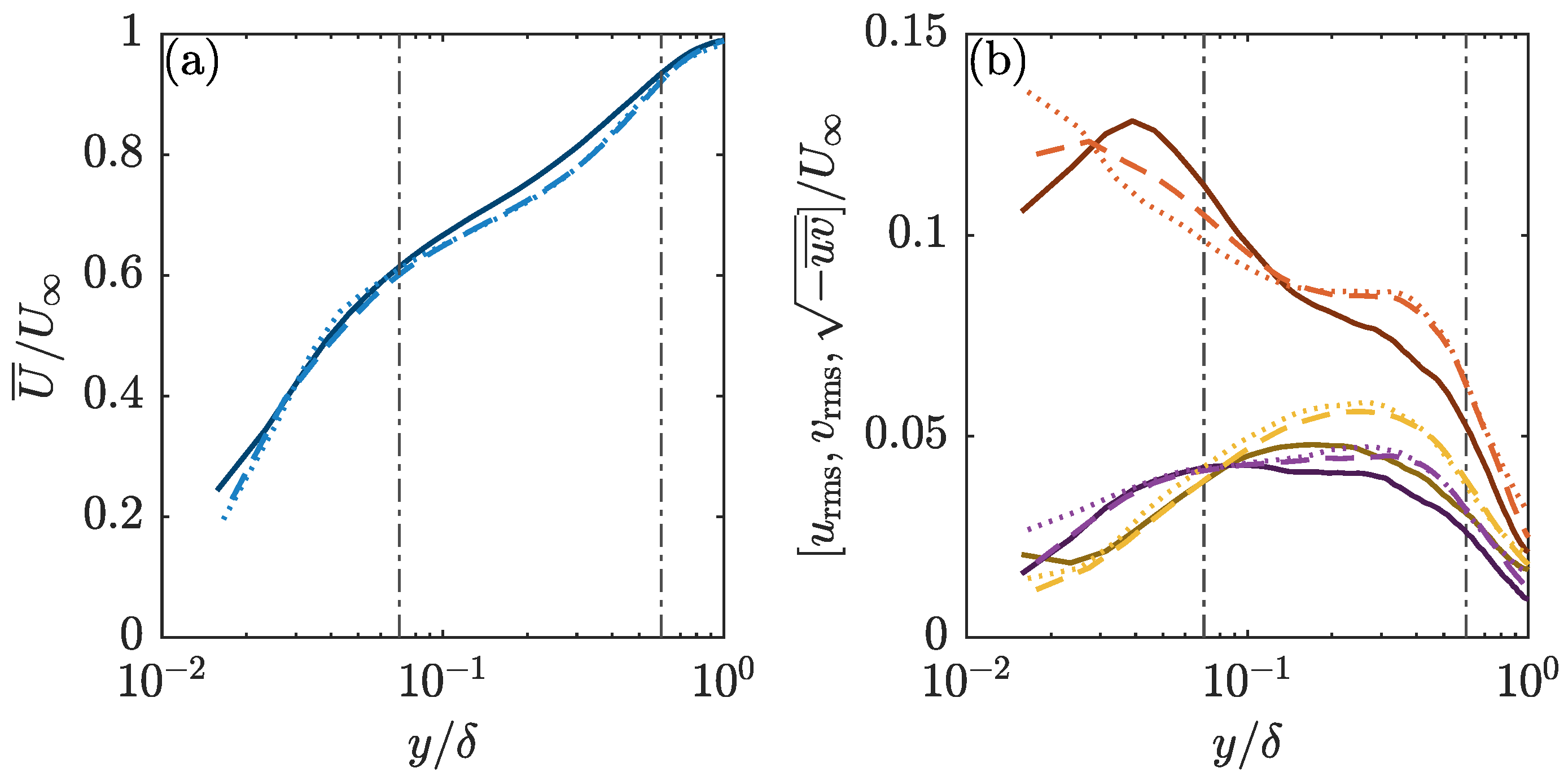
An important consideration in studying flows with compliant surfaces is whether the coupling is one-way or two-way. In a one-way coupling, the stresses in the flow deform the surface, but the deformations are small enough such that the mean flow properties are unaffected; this is typically taken to be for surface deformations less than 1 viscous unit [9]. For larger deformations, the influence of the surface on the flow must be considered. To investigate the level of coupling, the flow statistics are plotted in Figure 3 for the RW-DRF and CW-DRF data (from actuation condition iii), as well as the canonical data, taken from . In all of the profiles, the RW- and CW-DRF data agree well. For the mean velocity in Figure 3a, both profiles exhibit a deficit relative to the canonical case for . The turbulence intensities and Reynolds shear stress in Figure 3b are also similar between the RW and CW cases, having elevated energetics over the canonical profiles. Some deviation can be seen very near the wall, particularly in the . In addition, while very close to the rigid wall appears to exceed that for the compliant wall in apparent contrast to the findings of [5], this could be attributed to the differences in the parameters. More specifically, the study of Wang et al. [5], which identified a significant increase in near the wall, had similar levels of wall deformation in viscous scale while having significantly higher than our study. The study of Rosti and Brandt [8], at lower , showed no significant changes in the Reynolds stress tensor for the studied case with smallest wall deformation, which is still an order of magnitude larger in viscous scales compared with the measured wall deformation presented here. Overall, the effect of the elastic surface on the flow statistics appears to be minimal, suggesting that the system is in the one-way coupling regime. Though the compliant sample was made very soft, the one-way coupling may be explained by the low Reynolds number and thus low inertia of the flow.
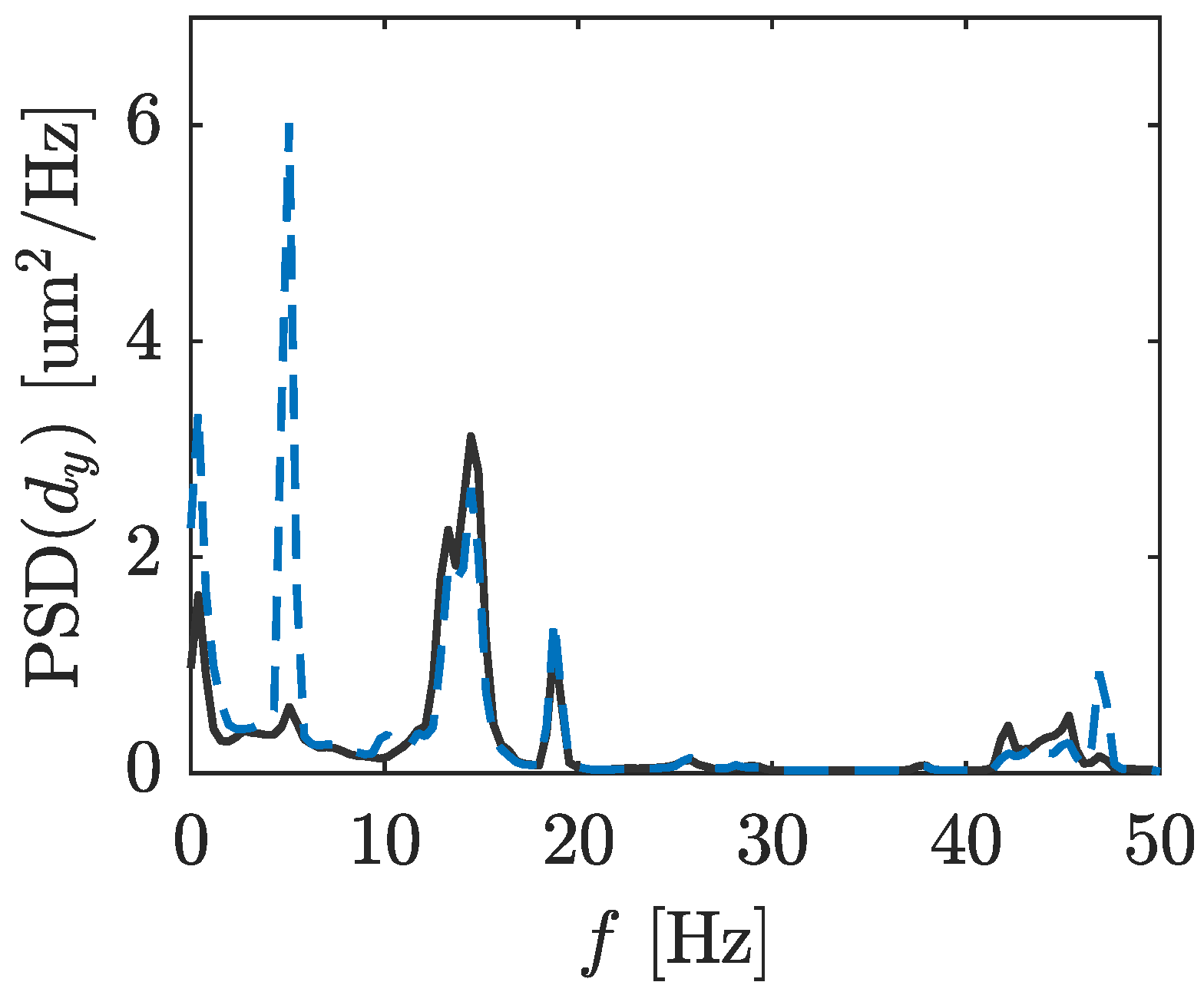
The mean properties of the flow contain the contributions of all length and timescales, and so for an effect of the surface to be observed in that context, it would have to be spectrally broadband, high in amplitude, or both. The use of the dynamic roughness as a deterministic input allows for a more focused analysis of more subtle interactions. Figure 4 shows temporal power spectra of the wall-normal deformation, , calculated using MATLAB’s pwelch function and averaged over the DIC field of view which was near the leading edge of the compliant sample. Given are the spectra for the CW-unforced and CW-DRF (actuation condition iii) studies. The two spectra are very similar in much of their spectral content, discussed in greater detail by Huynh and McKeon [15]. A slight difference is seen in the lowest resolvable frequency, but by far the most apparent distinction is the peak at 5 Hz for the DRF case, corresponding to the actuation frequency. Clearly the energy from the dynamic roughness is being transmitted to the gelatin, and without significantly modifying the spectral content from the unforced case.
3.2. Response to Forcing
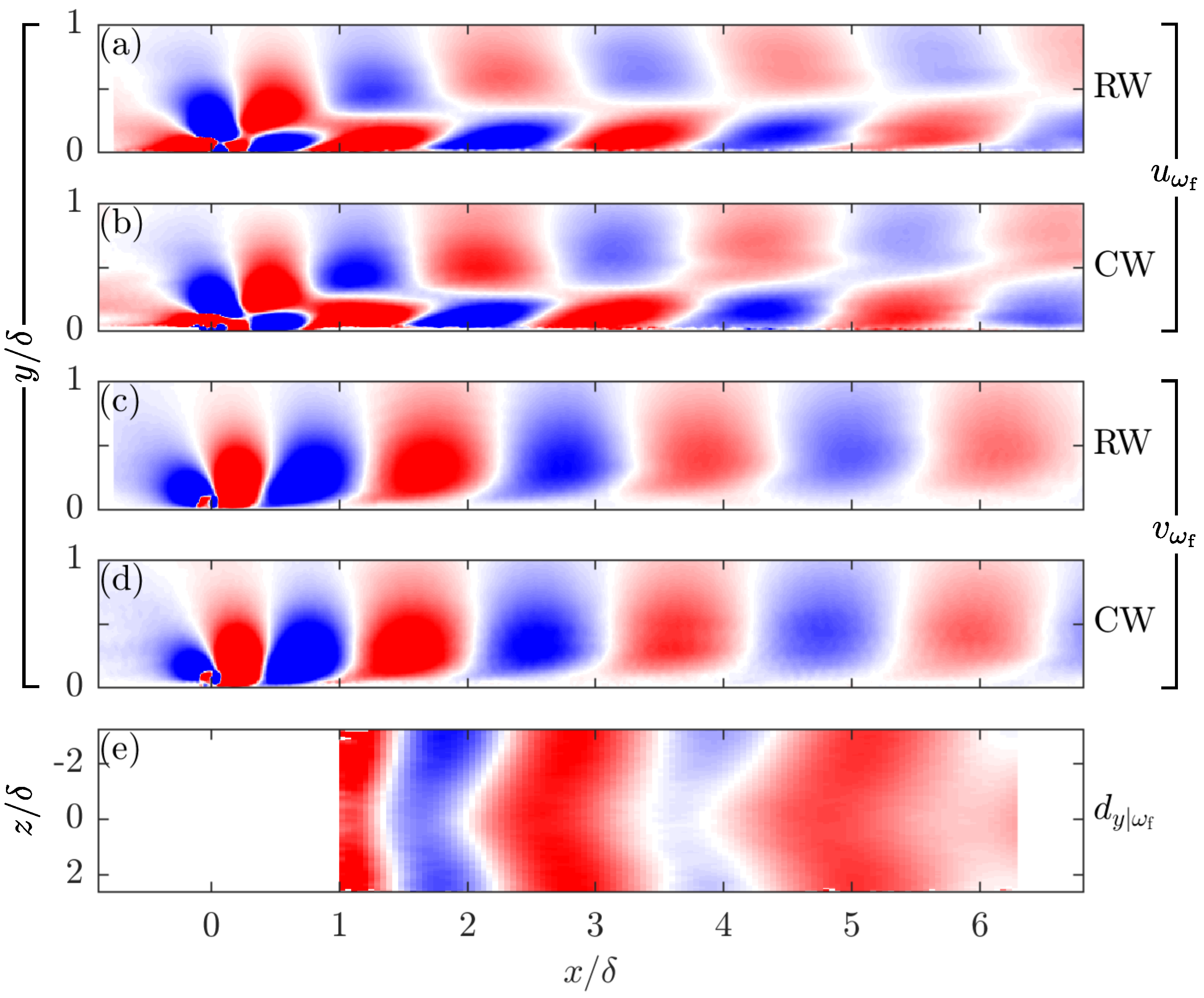
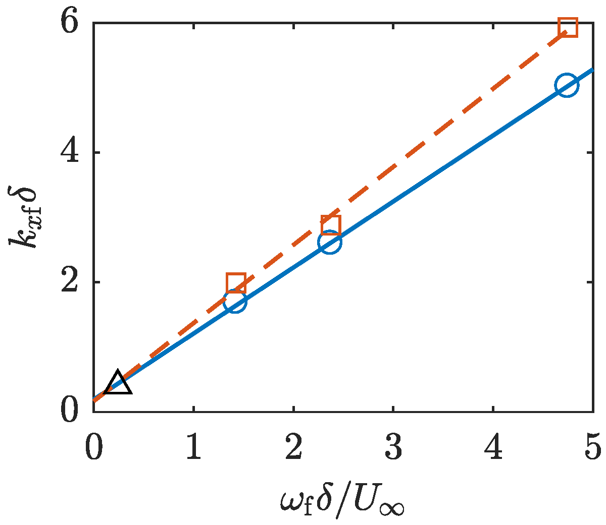
Further leveraging the synthetic input, the component coherent with the forcing frequency, , can be isolated from the velocity and deformation fields. This was done by a straightforward phase-averaging and discrete Fourier transform procedure in time [15]. is used to denote a quantity Fourier transformed in time and subscript indicates that only the () component has been retained. In Figure 5, the phase snapshots (corresponding to the roughness element lying flush with the wall) of the coherent RW-DRF and CW-DRF velocities and CW-DRF wall-normal deformation are presented, all from actuation condition iii. Looking at the velocity modes (a–d), the RW- and CW-DRF data once again compare well with one another. A streamwise periodic structure is immediately apparent in both and , and is seen to convect downstream while gradually decaying and drifting away from the wall. For both the RW and CW modes, undergoes a phase jump in y, while is tall and straight in y. This behavior is consistent with a two-dimensional perturbation. Under close inspection of the velocities near the downstream end of the measurement domain, the CW modes can be seen to lag slightly behind the RW modes. This apparent lag is due to the CW synthetic mode having a shorter streamwise lengthscale. Despite the two-dimensional nature of the mean characteristics of the boundary layer, we define an effective streamwise wavelength, , and effective streamwise wavenumber, , to compare the modes. This can be quantified by approximating the velocity mode as a streamwise-travelling wave and calculating the streamwise derivative of the mode phase to estimate [14]. Figure 6 shows the values calculated for actuation conditions i, ii, and iv, as well as the value for Duvvuri and McKeon [17]. The RW and CW data follow a linear trend over the frequency range explored, highlighted by the lines of best fit plotted alongside them. For all actuation conditions, the CW synthetic mode was found to have a higher value than the RW mode. This may be due to the compliant sample modifying the recirculation region just downstream of the roughness [26] and possibly reducing the convection velocity of the perturbation. Still, the general structure of the synthetic mode does not appear to be greatly affected by the compliant surface.
The coherent wall-normal deformation in Figure 5e contains a structure that is also streamwise periodic, although not as spanwise constant as the flow mode. There is a travelling wave component as well as a large-scale, high amplitude component that resembles a plate vibration mode. As discussed in Huynh and McKeon [15], the travelling wave content is distinct from other deformation features observed in the surface and is best attributed to a direct interaction with the synthetic flow mode. The bow to the otherwise spanwise constant structure corresponds closely to the slight spanwise variation of the flow mode [15]. The vibration-type mode was suggested to be the response of the gelatin to pressure fluctuations emanating from the roughness element, despite no physical contact between the roughness apparatus and the flat plate.
Using the value estimated from the velocity fields, the - travelling wave component was extracted from the signal using a discrete Fourier transform in x, with a zero-padding to spectrally interpolate to . is used to denote a quantity Fourier transformed in time and x, and subscript indicates that only the () component has been retained. The wall-normal deformation can then be related to the wall-normal velocity at the wall by the no-through boundary condition:
For actuation condition iii, the - deformation and wall velocity modes were estimated to be described by:
provides near-wall data that can be combined with PIV data to construct a complete picture of the synthetic flow mode as modified by the compliant surface.
3.3. Comparison of Experimental and Model Results
In the analysis thus far, the effect of the compliant wall on the flow has been minimal. Indeed, the root-mean-square (broadband) deformation is below 1 viscous unit and so a one-way coupling could be expected. Note that despite the small amplitude of the wall deformation, significant flow modification can occur due to the dynamic motion of a compliant wall, e.g., ref. [8,9,27], who identified associated changes to both the mean flow and turbulence structure, initiated at wall deformations smaller than one viscous unit. By taking advantage of the anticipated - travelling-wave content, we can investigate the interaction within the narrow context of the synthetic mode. Streamwise and wall-normal resolvent modes, and , were calculated using the rigid-wall () and compliant-wall () resolvent code. All resolvent modes were computed at , , matching the experimental results. The experimentally determined streamwise wavenumber was used for the rigid wall cases and for the compliant wall cases. However, the experimentally determined temporal frequency was not used in the resolvent for the following reasons. First of all, the temporal frequency is normalized using the friction velocity , which was difficult to accurately determine from the experimental results. Secondly, the resolvent modes are centered at the critical layer, where the phase speed ( under the quasi-streamwise parallel assumption being employed here) is equal to the local mean velocity. Although the difference between the mean profile used for the resolvent computation and the experimental mean profile did not change the resolvent mode shapes significantly, it had a non-negligible effect on the critical layer location. As a result, the phase speed of the resolvent modes were adjusted so that the location of the peak in the streamwise direction matched between the resolvent modes and the experimental results. The - Fourier modes from the experimental data were calculated as previous discussed.
The resolvent response modes with and without eddy viscosity and the experimental Fourier mode shapes are compared in Figure 7 for the rigid wall case and in Figure 8 for the compliant wall case. The mode amplitudes have been normalized by the peak in the corresponding streamwise mode amplitude, to preserve the relative amplitude information between () and (). The phase of the resolvent modes have been shifted such that at the streamwise peak location. The phase speeds in the rigid wall cases are for resolvent without eddy viscosity and for resolvent with eddy viscosity, these correspond to and , slightly lower than the reported from the experiments [15].
Although the - Fourier modes in Figure 7 and Figure 8 share many features with the resolvent modes without eddy viscosity, including the peak structure of the amplitudes, and the shapes of the mode phases, the resolvent analysis over-predicts the amplitude of the streamwise velocity perturbation compared with the wall-normal perturbation and under-predicts the wall normal height of the streamwise velocity peak. The resolvent with eddy viscosity improves the prediction of both the streamwise and wall-normal perturbations for the RW and CW cases, consistent with the results presented in previous work [28,29]. As for the phase information, Figure 8d shows a sharp deviation of the phase of and both the resolvent modes for the CW profile relative to the RW case. However, the variation is in the opposite sense, with consistent with a downstream tilted structure, while the resolvent modes with and without the eddy viscosity depict an upstream inclination. Still, the variation of the phase of suggests that a full jump might be observed if more near-wall data were available. Note that the expected phase of 1.19 for at the wall based on the deformation data in Equation (31) does not match particularly well with the CW profile, which attains a value of 1.45 at the lowest resolved point. This is not entirely surprising, as only the - coherent wall-normal deformation has been considered here. The other spatio-temporal scales may influence the observed phase of at the wall by inducing further wall deformation not accounted for here. Additionally, given the high water content of the gelatin, it is possible that the interface between the solid and fluid became semi-permeable, weakening the assumption of a no through-flow boundary condition.
Since the experimental results for RW and CW lead to the identification of different values, which strongly affects the peaks locations of the experimental Fourier modes, the RW and CW results are not compared directly with each other to determine the effect of the compliant wall. Instead, the resolvent modes with the same wavenumbers are used to isolate and identify the effect of the compliant wall in Figure 9.
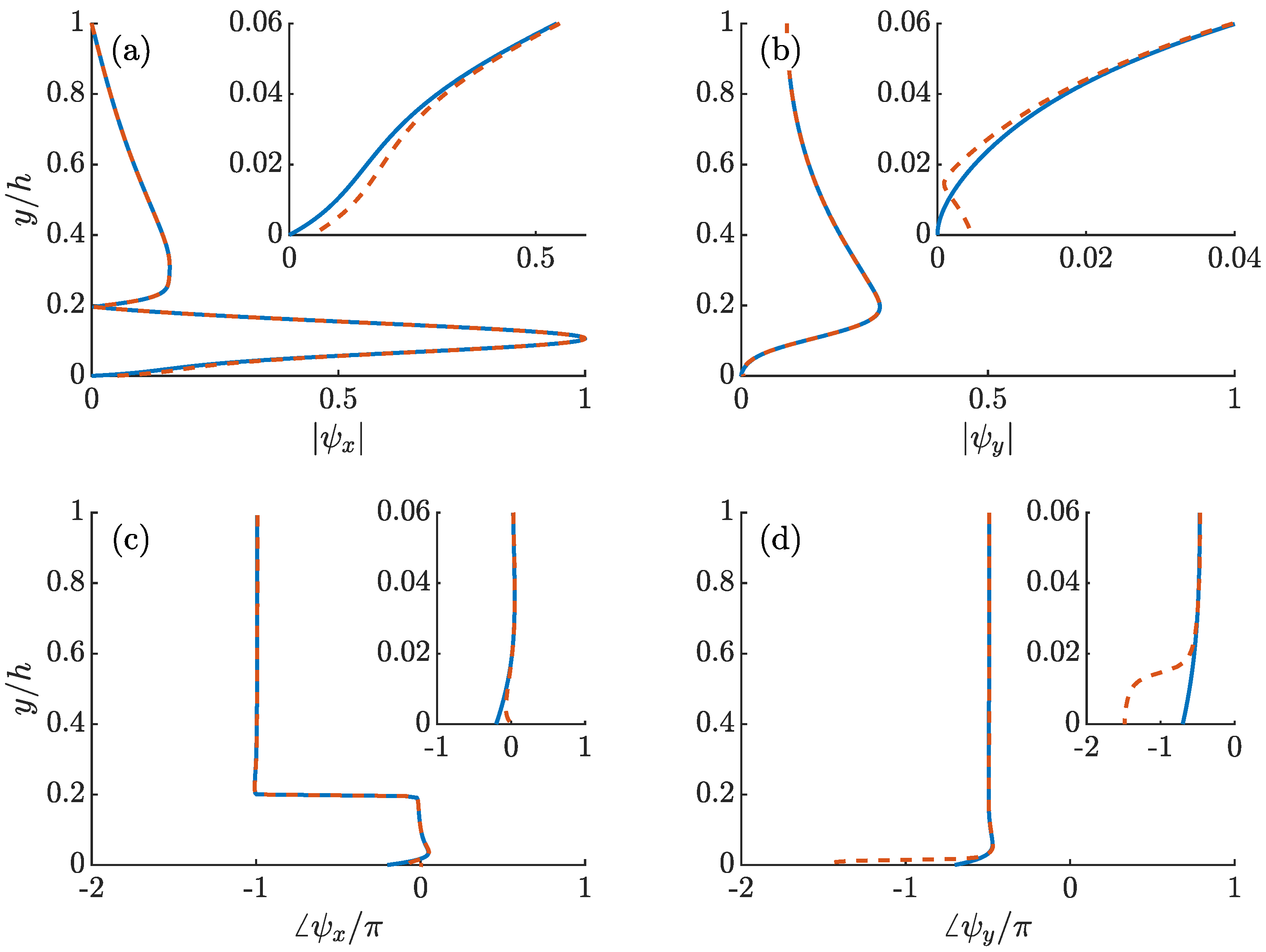
The compliant wall with wall-admittance is very close to a rigid wall; in the resolvent prediction in Figure 9, the RW and CW mode shapes match very well except in the near wall region. Very close to the wall, the amplitude of the streamwise resolvent mode for the CW deviates from the RW case and has a non-zero value at the wall as a result of the CW boundary condition given by Equation (11). For the wall-normal modes, has a jump very near the wall for the CW, while the RW mode has much less variation. This can be understood via the wall-admittance term in Equation (19). For a purely imaginary Y (with a positive imaginary part), the phase difference between and is required to be at the wall. Outside the near-wall region, and have been observed to have a nearly constant phase difference of [30]. Furthermore, Luhar et al. [30] showed that the pressure modes are essentially constant throughout the entire domain. Then in order to satisfy the phase boundary condition with an imaginary Y, is required to undergo a phase jump near the wall, as seen in the inset of Figure 9d. A signature can also be seen in the amplitude of , as shown in the inset of Figure 9b. Looking near , a local minimum is seen in , concurrent with the phase jump. These features were observed in previous resolvent-based opposition control studies [31]. From the perspective of the resolvent framework, the purely elastic wall mimics the action of the wall transpiration in an opposition control scheme, where wall jets oppose the vertical velocity at a detection plane near the wall, enforcing a phase jump and establishing a ‘virtual wall’.
Unlike the resolvent prediction, the near-wall amplitude of for the CW in the inset of Figure 8b does not exhibit a virtual wall signature. This may be due to the fact that a Fourier analysis in x assumes homogeneity in x. This is not strictly true, as the boundary layer flow is developing in the streamwise direction and, potentially more relevant, the gelatin sample was not perfectly smooth nor were the surface deformations limited to - waves.
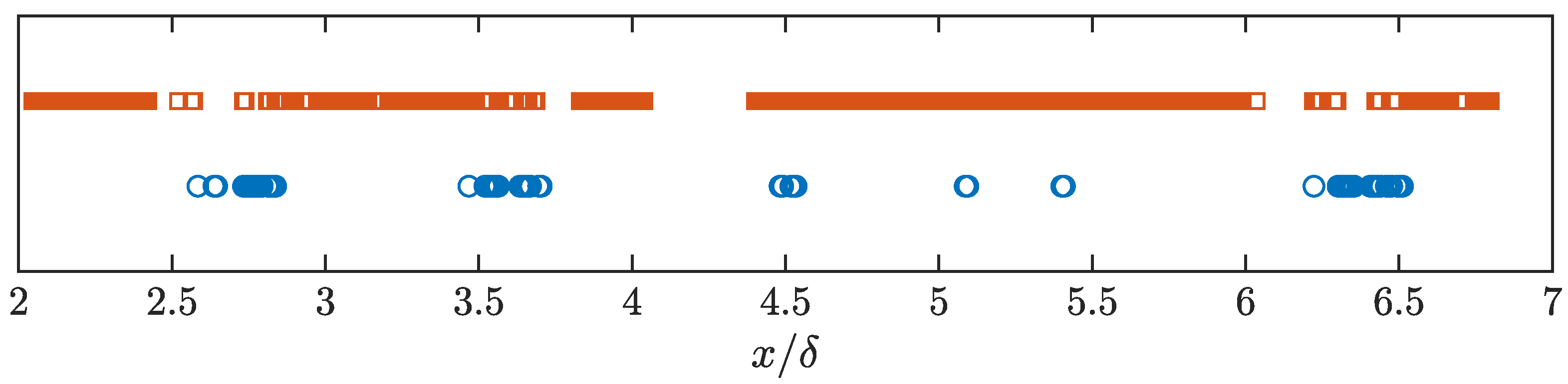
To circumvent the streamwise inhomogeneity of the flow and surface, a conditional average along x was devised based on the anticipated cusp feature of . The wall-normal gradient of was calculated at each streamwise location, the data were conditioned on whether the first three points from the wall had a negative gradient, i.e., . This condition was applied to both the RW and CW data for and for actuation condition iii to check for any systematic bias. The x locations where this condition was satisfied are plotted in Figure 10 for both the RW and CW data. 10% of the RW data met the criterion, while 64% of the CW data satisfied the condition. This statistically significant increase suggests a change to a physical structure close to the wall between the RW and CW cases.
Before averaging across observations in which the cusp criterion was satisfied, the cusp location was estimated by the near-wall zero-crossing of for each x. The profiles and were shifted in y such that the cusp point occurred at the same wall-normal location, . Finally, the shifted profiles were averaged together, yielding and . Note that phase information is lost in this process, while variation in the wall-normal locations of the cusplike features that would be masked in a simple averaging is retained. Efforts were made to develop an analogous procedure for the mode phases, but were hindered by noise in the data.
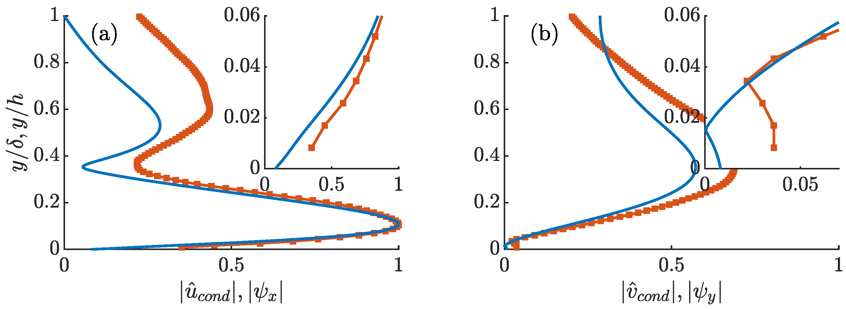
The conditionally averaged mode amplitudes for the CW case, and , are plotted in Figure 11 in comparison with the resolvent modes with eddy viscosity. They are nearly identical to the - Fourier mode amplitudes except in the near-wall region. The near-wall region of is shown in the insets of Figure 11b, where a clear cusp feature is now observed. The averaging procedure was conditioned on this feature, so its presence is not unexpected. However, the similarity to the mode is quite striking and is given more weight by 64% of the profiles containing this characteristic. The y-location and amplitude at the cusp of do not agree well with the resolvent predictions as shown in the inset of Figure 11b. This is at least partly due to the conditional averaging process that shifts the profiles at each x station in the wall-normal direction to line up the cusp locations, and also likely due to the spatial development of the boundary layer in the streamwise direction. Nonetheless, when combined with the observed phase variation of in Figure 8d, the experimental results confirm the conclusion from the resolvent analysis that the effect of the compliant wall on the synthetic flow mode is analogous to the sustenance of a virtual wall.
3.4. Compliant Wall as a Boundary Forcing
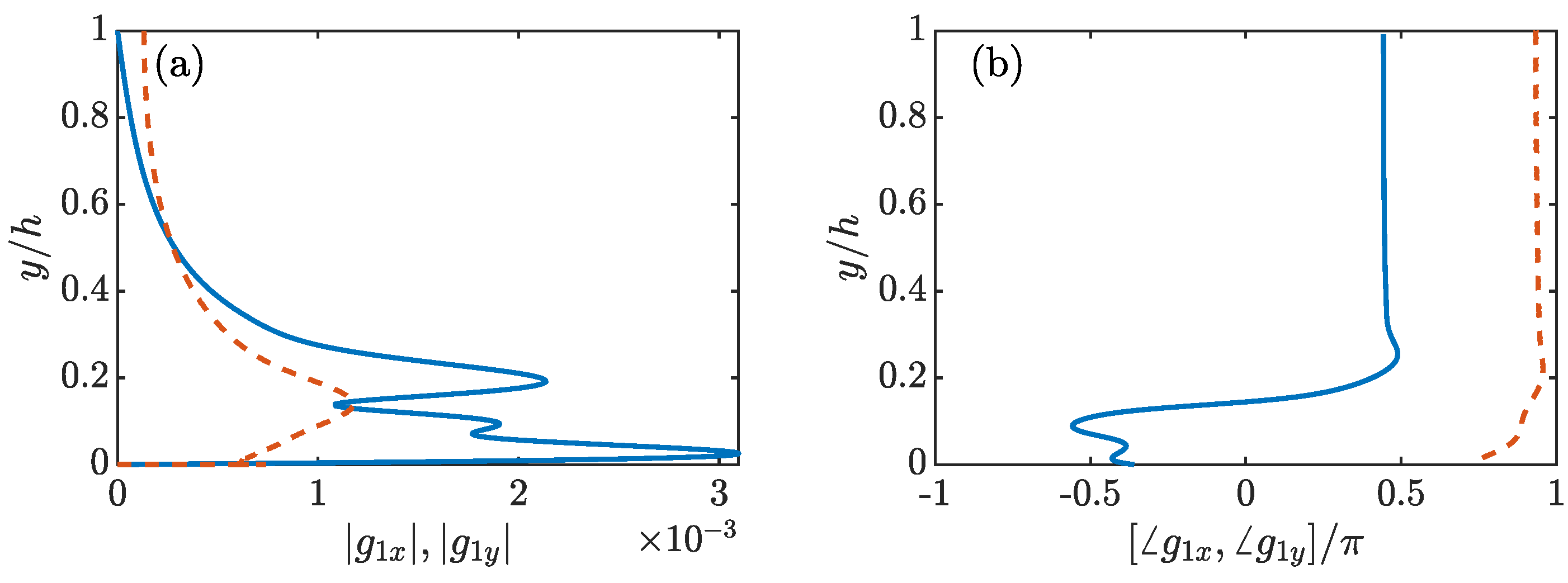
Turning back now to the treatment of the compliant wall boundary condition as a forcing to the rigid wall resolvent system, the amplitude and phase of the component of the boundary forcing for the relevant parameters of the experiment are plotted in Figure 12. As previously explained, the form of is not unique, and is therefore not plotted here. Because the wall with admittance of is close to being rigid, the changes due to the compliant wall boundary conditions are small, as observed previously in Figure 9. As a result, the magnitude of the component of the boundary forcing is very small.
In order to examine the effect of and , we will examine the change in response they induce, and , by plotting and comparing the magnitudes of three quantities in Figure 13. The first quantity is the non-normalized response for the RW case denoted as plotted in solid blue lines as reference. Additionally, the streamwise, spanwise velocities and the pressure of and , which capture the changes due to the and components of the boundary forcing are plotted. has very little effect on the response mode in the streamwise and spanwise directions, however, the wall pressure amplitude is increased by a small amount relative to the RW case. , on the other hand, accounts for most of the change in mode shape, including the non-zero boundary values and the local minimum in . As shown in Equation (28), arises because of the difference in the operator between the smooth and rough wall cases, , i.e., the difference in imposed boundary conditions.
As previously explained, the role of is to change the forcing mode shape to maximize the amplitude of the output, which is given by the singular value . For a case where the effect of the boundary condition is to reduce , acts to reduce the impact of that boundary condition. For example, in the case of a compliant wall that reduces , decreases the impact of the boundary condition by reducing the wall pressure to reduce wall deformation. On the contrary, in a case where the effect of the boundary condition is to increase , acts to increase the impact of that boundary condition. A reduction in the singular value can be used as a indication of drag reduction and vice versa, for example in the compliant wall studies of Luhar et al. [10] and Luhar et al. [24], and in the riblet studies of Chavarin and Luhar [32]. In these studies, the Fukagata–Iwamoto–Kasagi (FIK) identity [33] that is commonly used in drag reduction studies is used to describe the relationship between changes in the response mode shapes and the singular values to model drag reduction under idealized conditions. Therefore, can be interpreted as a term that acts to oppose drag reduction and assist drag increase. For the compliant wall with admittance of studied here, the boundary conditions increase the singular values, and Figure 13c shows that the amplitude of the pressure at the wall for is indeed higher than the RW case. Future work will explore more of the parameter space and attempt to draw more universal conclusions.
4. Discussion and Conclusions
This work utilized experiments and resolvent analysis to study the response of a compliant surface to the dynamic roughness forced synthetic mode in a turbulent boundary layer. Flow measurements were taken with 2D-PIV and surface deformation measured with stereo-DIC. The experimental Fourier modes were compared to resolvent modes with and without eddy viscosity and similar key features were observed. The resolvent modes highlighted the ‘virtual wall’ feature as a result of the compliant surface, identifying the change in near-wall structure of the resolvent modes arising from the change in boundary condition, and provided a method to model the effect of the boundary condition as an additional forcing.
The experimental measurements showed minimal difference in mean profile and flow statistics between the RW-DRF and CW-DRF cases and suggested a one-way coupling between the fluid and surface in the classical sense, or at least only mild changes relative to the rigid wall turbulence structure [5]. This may be the result of the low Reynolds number, therefore low inertia flow not causing enough surface deformation to create significant changes in the flow statistics. Indeed DIC measurements showed an rms surface deformation much smaller than the viscous length scale of the flow. On the other hand, the synthetic mode generated by the dynamic roughness introduced a strong peak in the power spectrum of the surface deformation at the forcing frequency , without significantly modifying the spectral content of other frequencies. This enabled a more focused analysis of the mode coherent with the forcing frequency. The measurements were Fourier transformed in time, and streamwise periodic structures were apparent in the components. Despite the two-dimensional nature of the mean characteristics of the boundary layer, the modes were approximated as streamwise-traveling waves. The dominant streamwise wavenumber was computed and the traveling wave component was extracted and compare with resolvent predictions.
The experimental Fourier modes for both the RW and CW cases were compared to the resolvent modes, which were computed under a number of relatively strong assumptions. The 1D resolvent analysis assumed a quasi-parallel flow, while the experimental measurements of the mode indicated a slowly developing boundary layer with decaying mode amplitude. However, as discussed in Jacobi and McKeon [16], the resolvent analysis can still capture significant features of the mode, with some discrepancies due to the non-parallel flow effects. Additionally, the mean profile used for the resolvent computations was a 1D channel mean profile generated using the eddy viscosity model. The difference between the mean profile used for the resolvent analysis and that observed in the experiments did not significantly change the mode shapes except in the outer region of the flow where the influence of the semi-infinite boundary layer domain is important. However, later results indicated that the effect of the compliant wall with small admittance parameter Y resulted in changes only in regions very close to the wall, which was the focus of most of the analysis. The same mean profile was used for both the RW and CW resolvent mode computations, which can be justified by the one-way fluid-surface coupling confirmed by the small surface deformation measurements and the small differences in the measured mean profiles for both cases. Together, these simplifications significantly reduced the costs for the resolvent computation while still capturing the most significant aspects of the structure of the modes. The comparison between the experimental and model responses of the flow to the synthetic excitation by dynamic roughness for the RW and CW cases demonstrate that resolvent analysis is capable of identifying the type of near-wall changes that may underlie the observations of changes to turbulence structure for even sub-viscous-scale wall deformations [5,8,9], a topic for future work.
Although the resolvent analysis captured the trends of the experimental Fourier modes, the addition of an eddy viscosity improved the agreement with the experiment. The resolvent modes with eddy viscosity improved the mode shape of the streamwise velocity, and increased the energy in the wall-normal direction, consistent with previous results in Symon et al. [29] and Illingworth et al. [28]. As for the compliant wall modes, both resolvent with and without eddy viscosity predicted a virtual wall signature in the wall-normal velocity, stemming from the purely imaginary wall admittance (corresponding to a purely elastic surface). This was used to construct a conditional average that revealed the virtual wall feature in the experimental data, a subtle detail that would have been difficult to identify without the lens of an accurate model. The data and model prediction suggest that the elastic compliant surface acts to oppose the wall-normal velocity of the synthetic flow mode near the wall, in a manner similar to opposition control. The fact that this modification did not readily appear in the flow statistics indicates that the contributions of other prevailing flow scales must be accounted for, leaving the door open for continued development of the resolvent-based framework.
Additionally, the resolvent analysis led to a method of modeling the effect of the boundary conditions as an extra forcing. The terms contributing to the boundary forcing were split into a term that is the result of the change in forcing mode, and a term that is the direct result of the change in boundary conditions. Detailed analysis showed that opposes (assists) the effect of the change in boundary conditions when the singular values are being decreased (increased). The method presented here can potentially be used for simplifying future numerical studies, especially eddy resolved simulations. For example, previous work by Varghese and Durbin [34] represented the effect of the surface roughness with a drag force in eddy resolving simulations. The drag force, which was quadratic in velocity and confined to a zone next to the wall, was able to capture the dominant effects of roughness geometries. However, the drag constant in the model was selected to match the skin friction of a simulation with roughness geometry. Motivated by this result, the formulation of the boundary forcing presented here can potentially provide information about the forcing required to capture the effects of certain boundary conditions a priori, although several questions remain for future studies, including methods to generalize the linear boundary conditions to more general surface features, the selection of the resolvent mode weights, and interactions between modes with different wavenumbers.
In conclusion, the disparity in the respective costs of performing a challenging experimental campaign on a turbulent boundary layer over a compliant wall with deterministic forcing over a period of many months, and the 1D resolvent analysis, which runs in seconds on a standard laptop, underscores the utility of this tool for design of passive (and active) control strategies for turbulent flows.
Author Contributions
Conceptualization, D.P.H. and B.J.M.; methodology, D.P.H., Y.H. and B.J.M.; investigation, D.P.H. and Y.H.; writing, D.P.H., Y.H. and B.J.M.; supervision, B.J.M.; funding acquisition, B.J.M. All authors have read and agreed to the published version of the manuscript.
Funding
The support of the U.S. Office of Naval Research under grant number N00014-17-1-2960 and the U.S. Army Research Office under W911NF-17-1-0306 is gratefully acknowledged.
Institutional Review Board Statement
Not applicable.
Informed Consent Statement
Not applicable.
Data Availability Statement
The data reported here are available on request.
Conflicts of Interest
The authors declare no conflict of interest. The funders had no role in the design of the study; in the collection, analyses, or interpretation of data; in the writing of the manuscript, or in the decision to publish the results.
Abbreviations
The following abbreviations are used in this manuscript:
| CW | Compliant wall |
| DIC | Digital Image Correlation |
| DNS | Direct Numerical Simulation |
| DRF | Dynamic roughness forced |
| PIV | Particle Image Velocimetry |
| RW | Rigid wall |
References
- Gad-el Hak, M. Flow Control: Passive, Active and Reactive Flow Management; Cambridge University Press: Cambridge, UK, 2000. [Google Scholar]
- Gad-el Hak, M. Compliant coatings for drag reduction. Prog. Aero. Sci. 2002, 38, 77–99. [Google Scholar] [CrossRef]
- Lee, T.; Fisher, M.; Schwarz, W. Investigation of the stable interaction of a passive compliant surface with a turbulent boundary layer. J. Fluid Mech. 1993, 257, 373–401. [Google Scholar] [CrossRef]
- Choi, K.; Yang, X.; Clayton, B.; Glover, E.; Atlar, M.; Semenov, B.; Kulik, V. Turbulent drag reduction using compliant surfaces. Proc. R. Soc. A 1997, 453, 2229–2240. [Google Scholar] [CrossRef]
- Wang, J.; Koley, S.S.; Katz, J. On the interaction of a compliant wall with a turbulent boundary layer. J. Fluid Mech. 2020, 899, A20. [Google Scholar] [CrossRef]
- Xu, S.; Rempfer, D.; Lumley, J. Turbulence over a compliant surface: Numerical simulation and analysis. J. Fluid Mech. 2003, 478, 11–34. [Google Scholar] [CrossRef] [Green Version]
- Fukagata, K.; Kern, S.; Chatelain, P.; Koumoutsakos, P.; Kasagi, N. Evolutionary optimization of an anisotropic compliant surface for turbulent friction drag reduction. J. Turb. 2008, 35, 1–17. [Google Scholar] [CrossRef]
- Rosti, M.E.; Brandt, L. Numerical simulation of turbulent channel flow over a viscous hyper-elastic wall. J. Fluid Mech. 2017, 830, 708–735. [Google Scholar] [CrossRef] [Green Version]
- Benschop, H.; Greidanus, A.; Delfos, R.; Westerweel, J.; Breugem, W.P. Deformation of a linear viscoelastic compliant coating in a turbulent flow. J. Fluid Mech. 2019, 859, 613–658. [Google Scholar] [CrossRef] [Green Version]
- Luhar, M.; Sharma, A.; McKeon, B. A framework for studying the effect of compliant surfaces on wall turbulence. J. Fluid Mech. 2015, 768, 415–441. [Google Scholar] [CrossRef] [Green Version]
- McKeon, B.; Sharma, A. A critical-layer framework for turbulent pipe flow. J. Fluid Mech. 2010, 658, 336–382. [Google Scholar] [CrossRef] [Green Version]
- McKeon, B.J. The engine behind (wall) turbulence: Perspectives on scale interactions. J. Fluid Mech. 2017, 817. [Google Scholar] [CrossRef] [Green Version]
- Jovanovic, M. From bypass transition to flow control and data-driven turbulence modeling: An input-output viewpoint. Annu. Rev. Fluid Mech. 2021, 53, 311–345. [Google Scholar] [CrossRef]
- Huynh, D.; McKeon, B. Characterization of the spatio-temporal response of a turbulent boundary layer to dynamic roughness. Flow Turb. Comb. 2020, 104, 293–316. [Google Scholar] [CrossRef]
- Huynh, D.; McKeon, B. Measurements of a turbulent boundary layer-compliant surface system in response to targeted, dynamic roughness forcing. Expts. Fluids 2020, 61, 94. [Google Scholar] [CrossRef]
- Jacobi, I.; McKeon, B. Dynamic roughness perturbation of a turbulent boundary layer. J. Fluid Mech. 2011, 688, 258–296. [Google Scholar] [CrossRef] [Green Version]
- Duvvuri, S.; McKeon, B. Triadic scale interactions in a turbulent boundary layer. J. Fluid Mech. 2015, 767. [Google Scholar] [CrossRef]
- McKeon, B.; Jacobi, I.; Duvvuri, S. Dynamic roughness for manipulation, control of turbulent boundary layers: An overview. AIAA J. 2018, 56, 2178–2193. [Google Scholar] [CrossRef]
- Gad-el Hak, M. The response of elastic and viscoelastic surfaces to a turbulent boundary layer. J. Appl. Mech. 1986, 53, 206–212. [Google Scholar] [CrossRef]
- Czerner, M.; Fellay, L.; Suárez, M.; Frontini, P.; Fasce, L. Determination of elastic modulus of gelatin gels by indentation experiments. Proc. Mat. Sci. 2015, 8, 287–296. [Google Scholar] [CrossRef] [Green Version]
- Del Álamo, J.C.; Jiménez, J. Linear energy amplification in turbulent channels. J. Fluid Mech. 2006, 559, 205. [Google Scholar] [CrossRef] [Green Version]
- Hwang, Y.; Cossu, C. Linear non-normal energy amplification of harmonic and stochastic forcing in the turbulent channel flow. J. Fluid Mech. 2010, 664, 51–73. [Google Scholar] [CrossRef] [Green Version]
- Reynolds, W.; Hussain, A. The mechanics of an organized wave in turbulent shear flow. Part 3. Theoretical models and comparisons with experiments. J. Fluid Mech. 1972, 54, 263–288. [Google Scholar] [CrossRef]
- Luhar, M.; Sharma, A.; McKeon, B. On the design of optimal compliant walls for turbulence control. J. Turb. 2016, 17, 787–806. [Google Scholar] [CrossRef] [Green Version]
- Saxton-Fox, T.; McKeon, B. Coherent structures, uniform momentum zones and the streamwise energy spectrum in wall-bounded turbulent flows. J. Fluid Mech. 2017, 826. [Google Scholar] [CrossRef]
- Jacobi, I.; McKeon, B. New perspectives on the impulsive roughness-perturbation of a turbulent boundary layer. J. Fluid Mech. 2011, 677, 179–203. [Google Scholar] [CrossRef] [Green Version]
- Kim, E.; Choi, H. Space-time characteristics of a compliant wall in a turbulent channel flow. J. Fluid Mech. 2014, 756, 30–53. [Google Scholar] [CrossRef]
- Illingworth, S.J.; Monty, J.P.; Marusic, I. Estimating large-scale structures in wall turbulence using linear models. J. Fluid Mech. 2018, 842, 146–162. [Google Scholar] [CrossRef] [Green Version]
- Symon, S.; Illingworth, S.J.; Marusic, I. Energy transfer in turbulent channel flows and implications for resolvent modelling. J. Fluid Mech. 2021, 911, A3. [Google Scholar] [CrossRef]
- Luhar, M.; Sharma, A.; McKeon, B. On the structure and origin of pressure fluctuations in wall turbulence: Predictions based on the resolvent analysis. J. Fluid Mech. 2014, 751, 38–70. [Google Scholar] [CrossRef] [Green Version]
- Luhar, M.; Sharma, A.; McKeon, B. Opposition control within the resolvent analysis framework. J. Fluid Mech. 2014, 749, 597–626. [Google Scholar] [CrossRef] [Green Version]
- Chavarin, A.; Luhar, M. Resolvent analysis for turbulent channel flow with riblets. AIAA J. 2020, 58, 589–599. [Google Scholar] [CrossRef] [Green Version]
- Fukagata, K.; Iwamoto, K.; Kasahi, N. Contribution of Reynolds stress distribution to the skin friction in wall-bounded flows. Phys. Fluids 2002, 14, 73–76. [Google Scholar] [CrossRef] [Green Version]
- Varghese, J.; Durbin, P.A. Representing surface roughness in eddy resolving simulation. J. Fluid Mech. 2020, 897, A10. [Google Scholar] [CrossRef]
Figure 1.
Illustration of the experimental setup. The rectangles representing the PIV fields are not true to scale or aspect ratio, but represent the FOVs of the two cameras and the streamwise shift (green locations to blue locations) between setups required to obtain the long spatial field of view reported here. The phase-averaged vector fields were stitched together in post-processing. Mean statistics are reported from , and streamwise locations of the LE and TE of the compliant panel are also shown. The illustration is vertically reflected relative to the physical setup, i.e., measurements are made on the bottom surface of the flat plate.

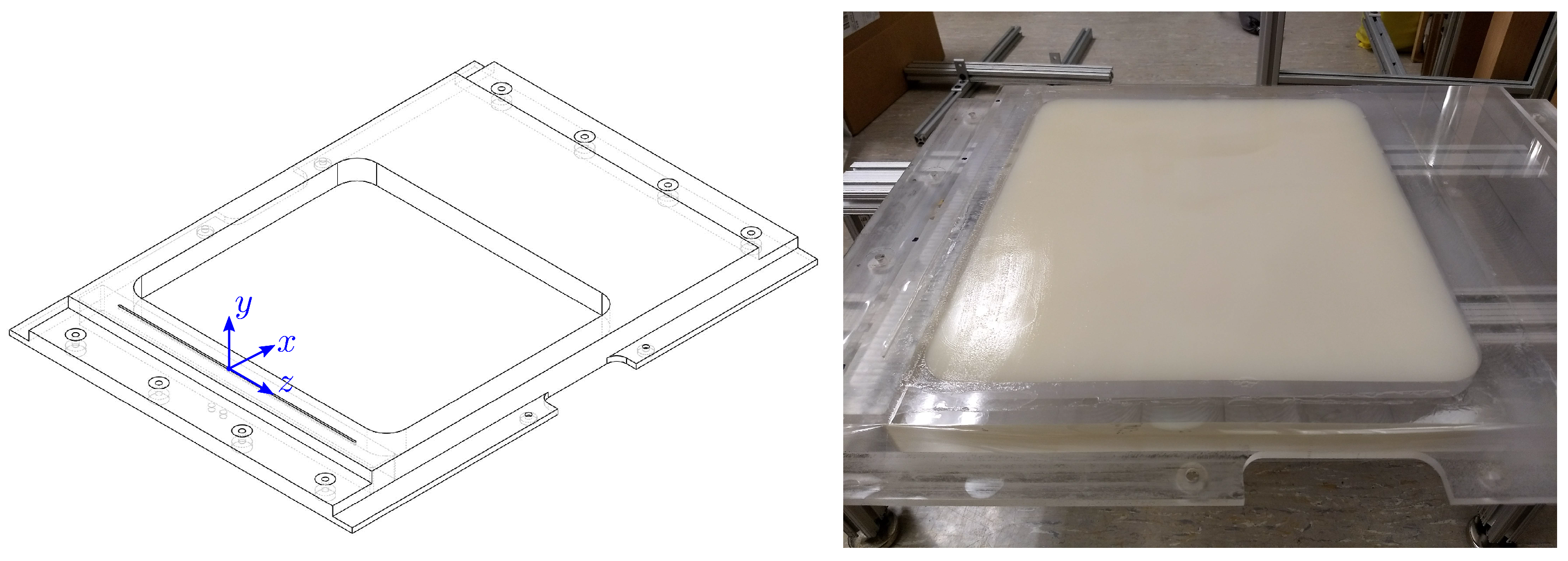
Figure 2.
Schematic of dynamic roughness slot (at ) and the compliant wall insert (left) and a finished gelatin sample (right). Note the sample pictured was dyed white for a DIC test. The gelatin used in the experiments was translucent.
Figure 2.
Schematic of dynamic roughness slot (at ) and the compliant wall insert (left) and a finished gelatin sample (right). Note the sample pictured was dyed white for a DIC test. The gelatin used in the experiments was translucent.

Figure 3.
Comparison of the RW-DRF, CW-DRF (both from actuation condition iii), and canonical mean flow statistics (): (a) mean streamwise velocity (blue), (b) streamwise (red) and wall-normal (yellow) turbulence intensities, and Reynolds shear stress (purple). Line styles are as follows: (solid) canonical, (dashed) RW-DRF, (dotted) CW-DRF. The vertical dash-dotted lines indicate .

Figure 4.
Comparison of the power spectra of the wall-normal deformation, , between the unforced (solid) and forced (dashed) studies. Data correspond to the leading-edge FOV and have been spatially-averaged over x and z.
Figure 4.
Comparison of the power spectra of the wall-normal deformation, , between the unforced (solid) and forced (dashed) studies. Data correspond to the leading-edge FOV and have been spatially-averaged over x and z.

Figure 5.
Phase snapshots () of the RW-DRF and CW-DRF coherent (a–d) velocity and (e) wall-normal deformation fields, all from actuation condition iii. For the velocities, the (a,c) RW rigid- and (b,d) SW smooth-wall data are given for comparison, and the contour shading limits are (red/blue indicate high/low speed). For the wall-normal deformation, the contour shading limits are um.

Figure 6.
Streamwise wavenumber of the synthetic mode, , plotted against angular forcing frequency, , for actuation amplitude : ◯ RW-DRF data; — RW-DRF linear fit, ; □ CW-DRF data; – – CW-DRF linear fit, ; △ Duvvuri and McKeon [17].
Figure 6.
Streamwise wavenumber of the synthetic mode, , plotted against angular forcing frequency, , for actuation amplitude : ◯ RW-DRF data; — RW-DRF linear fit, ; □ CW-DRF data; – – CW-DRF linear fit, ; △ Duvvuri and McKeon [17].

Figure 7.
Comparison of the (a,b) amplitude and (c,d) phase between the experimental results (red solid lines with circle markers), the resolvent modes (blue dash lines), and the resolvent modes with eddy viscosity (blue solid lines) for the rigid wall case. Figures (a,c) are the streamwise modes, and (b,d) are the wall-normal modes. Markers for the experimental results indicate locations where measurements were taken. Mode amplitudes are normalized by their peak streamwise amplitude, and phases are matched at the peak location. Insets are the near wall close-up views for . Parameters for resolvent analysis are , and , without and with eddy viscosity, respectively.

Figure 8.
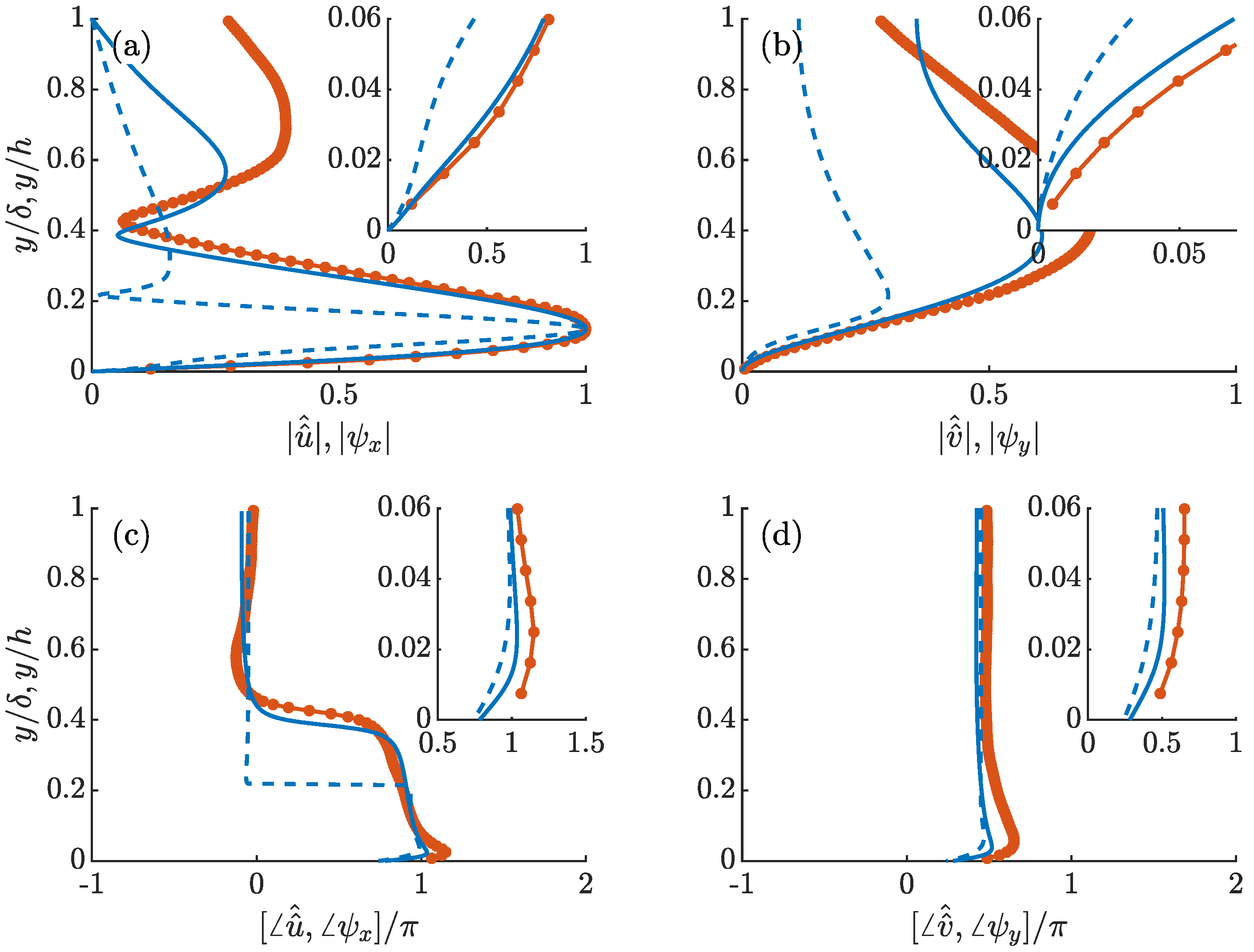
Comparison of the (a,b) amplitude and (c,d) phase between the experimental results (red solid lines with circle markers), the resolvent modes (blue dash lines), and the resolvent modes with eddy viscosity (blue solid lines) for the compliant wall. Figures (a,c) are the streamwise modes, and (b,d) are the wall-normal modes. Markers for the experimental results indicate locations where measurements were taken. Mode amplitudes are normalized by their peak streamwise amplitude, and phases are matched at the peak location. Insets are the near wall close-up views for . Parameters for the resolvent analysis are , and , without and with eddy viscosity, respectively.
Figure 8.
Comparison of the (a,b) amplitude and (c,d) phase between the experimental results (red solid lines with circle markers), the resolvent modes (blue dash lines), and the resolvent modes with eddy viscosity (blue solid lines) for the compliant wall. Figures (a,c) are the streamwise modes, and (b,d) are the wall-normal modes. Markers for the experimental results indicate locations where measurements were taken. Mode amplitudes are normalized by their peak streamwise amplitude, and phases are matched at the peak location. Insets are the near wall close-up views for . Parameters for the resolvent analysis are , and , without and with eddy viscosity, respectively.

Figure 9.
Comparison of the resolvent modes in the (a,c) the streamwise direction , (b,d) wall-normal direction between the rigid wall (blue solid lines) and compliant wall (red dash lines). Figures (a,b) are mode amplitudes, and (c,d) are mode phases. The resolvent parameters are , for both cases. Mode amplitudes are normalized by their peak values, and phases are set to zero at the critical layer. Insets are the near wall close-up views for .

Figure 10.
A visualization of the streamwise locations where the near-wall condition is met for the compliant wall experiment (red squares on the top line), and the rigid wall experiment (blue circles on the bottom line).
Figure 10.
A visualization of the streamwise locations where the near-wall condition is met for the compliant wall experiment (red squares on the top line), and the rigid wall experiment (blue circles on the bottom line).

Figure 11.
Comparison of the amplitude between the conditional averaged experimental results (red solid lines with square markers), and the resolvent mode with eddy viscosity (blue solid lines) for the compliant wall. Figure (a) is the streamwise modes, and figure (b) is the wall-normal modes. Markers for the experimental results indicate locations where measurements were taken. Mode amplitudes are normalized by their peak streamwise amplitude. Insets are the near wall close-up views for . Parameters for resolvent with eddy viscosity are .

Figure 12.
The (a) amplitude and (b) phase of the component of the boundary induced forcing. Blue solid line is the streamwise direction forcing and red dash line is the wall-normal direction forcing . The parameters are , and for the compliant wall with .
Figure 12.
The (a) amplitude and (b) phase of the component of the boundary induced forcing. Blue solid line is the streamwise direction forcing and red dash line is the wall-normal direction forcing . The parameters are , and for the compliant wall with .

Figure 13.
The amplitude of (blue solid lines), (red dash lines), and (yellow dash dot lines) in the near wall region of . Subplots from left to right are (a) the streamwise response mode , (b) the spanwise response mode and (c) the pressure response mode . Parameters are , , .
Figure 13.
The amplitude of (blue solid lines), (red dash lines), and (yellow dash dot lines) in the near wall region of . Subplots from left to right are (a) the streamwise response mode , (b) the spanwise response mode and (c) the pressure response mode . Parameters are , , .


Table 1.
Mean properties of the canonical flow, acquired at 63 cm downstream of the leading edge: freestream velocity, friction velocity, (99%) boundary layer thickness, viscous unit , eddy turnover time , Reynolds numbers based on momentum thickness, , and friction Reynolds number, .
Table 1.
Mean properties of the canonical flow, acquired at 63 cm downstream of the leading edge: freestream velocity, friction velocity, (99%) boundary layer thickness, viscous unit , eddy turnover time , Reynolds numbers based on momentum thickness, , and friction Reynolds number, .
| [cm/s] | [cm/s] | [mm] | [um] | [s] | ||
|---|---|---|---|---|---|---|
| 33 | 1.6 | 25.5 | 62.5 | 0.077 | 870 | 410 |
Table 2.
Dynamic roughness actuation conditions (i–iv) explored in these experiments: dimensional, and non-dimensional quantities parameterized by motion rms height and frequency given.
Table 2.
Dynamic roughness actuation conditions (i–iv) explored in these experiments: dimensional, and non-dimensional quantities parameterized by motion rms height and frequency given.
| i | ii | iii | iv | |
|---|---|---|---|---|
| 3 Hz | 5 Hz | 5 Hz | 10 Hz | |
| 1.1 mm | 1.1 mm | 1.8 mm | 1.1 mm | |
| 1.4 | 2.4 | 2.4 | 4.8 | |
| 0.042 | 0.042 | 0.069 | 0.042 |
Publisher’s Note: MDPI stays neutral with regard to jurisdictional claims in published maps and institutional affiliations. |
© 2021 by the authors. Licensee MDPI, Basel, Switzerland. This article is an open access article distributed under the terms and conditions of the Creative Commons Attribution (CC BY) license (https://creativecommons.org/licenses/by/4.0/).
Share and Cite
MDPI and ACS Style
Huynh, D.P.; Huang, Y.; McKeon, B.J. Experiments and Modeling of a Compliant Wall Response to a Turbulent Boundary Layer with Dynamic Roughness Forcing. Fluids 2021, 6, 173. https://0-doi-org.brum.beds.ac.uk/10.3390/fluids6050173
AMA Style
Huynh DP, Huang Y, McKeon BJ. Experiments and Modeling of a Compliant Wall Response to a Turbulent Boundary Layer with Dynamic Roughness Forcing. Fluids. 2021; 6(5):173. https://0-doi-org.brum.beds.ac.uk/10.3390/fluids6050173
Chicago/Turabian StyleHuynh, David P., Yuting Huang, and Beverley J. McKeon. 2021. "Experiments and Modeling of a Compliant Wall Response to a Turbulent Boundary Layer with Dynamic Roughness Forcing" Fluids 6, no. 5: 173. https://0-doi-org.brum.beds.ac.uk/10.3390/fluids6050173