
Study of Different Alternatives for Dynamic Simulation of a Steam Generator Using MATLAB


Mechanical Engineering Department, Universidad Francisco de Paula Santander, Vía Acolsure, Sede el Algodonal Ocaña, Ocaña 546552, Colombia
*
Authors to whom correspondence should be addressed.
Fluids 2021, 6(5), 175; https://0-doi-org.brum.beds.ac.uk/10.3390/fluids6050175
Submission received: 5 April 2021
/
Revised: 24 April 2021
/
Accepted: 26 April 2021
/
Published: 29 April 2021
(This article belongs to the Special Issue Advances in Numerical Methods for Multiphase Flows, Volume II)
Abstract
:This work presents the simulation of a steam generator or water-tube boiler through the implementation in MATLAB® for a proposed mathematical model. Mass and energy balances for the three main components of the boiler—the drum, the riser and down-comer tubes—are presented. Three alternative solutions to the ordinary differential equation (ODE) were studied, based on Runge–Kutta 4th order method, Heun’s method, and MATLAB function Ode45. The best results were obtained using MATLAB® function Ode45 based on the Runge–Kutta 4th Order Method. The error was less than 5% for the simulation of the steam pressure in the drum, the total volume of water in the boiler, and the mixture quality in relation to what was reported.
1. Introduction
The world should prepare for the demand for energy to skyrocket in the next 20 years. By 2040, it will rise by 30% with an annual growth rate of 1.4% [1]. This growth will be like adding another China and India to global demand, warns the annual report of the International Energy Agency (IEA). The IEA indicates that the global economy is growing at an average rate of 3.4% per year. Additionally, the IEA estimates that the population will expand from 7.4 billion to 9 billion people by 2040, and there will be an urbanization process that will add the equivalent of a city the size of Shanghai to the world’s urban population every four months. The energy sector will experience profound changes, with new production powers and a shift in energy sources that will supply energy to humanity.
For these reasons, the energy supply on the planet can be considered a major concern for all countries. In addition, most energy production is carried out with fossil fuels, along with the environmental problems associated with their use, such as global warming, air pollution, and acid rain [2].
One of the most feasible strategies to mitigate the impact generated by the use of fossil fuels in power generation is to improve the efficiency of power plants. The efficient operation of steam generators or boilers is indispensable for the correct functioning of this type of plant known as thermal power plants. The boiler is responsible for transforming the chemical energy of a fuel such as coal, oil, gas, or nuclear energy into thermal energy, using this heat to convert water into steam [3].
The steam generator is used in the oil [4], pharmaceutical [5], and thermoelectric industries, among others. It is necessary to know and understand the functioning of these systems. This has been possible through the formulation of mathematical models that represent their behavior with excellent results [6,7,8,9,10,11,12].
Recent studies have used the mathematical model defined by ordinary differential equations (ODEs) [6]. They used this model to simulate the behavior of thermal power plants with heat recovery systems. This is the case of the works that reported the dynamic behavior of key parameters involved in the steam generation process, such as the appropriate rate of water and fuel consumption according to the rate of heat required in the boiler risers [13]. Other studies reported the response of water consumption and steam generation in the boiler, based on the variables of water level, pressure, and mixture quality in the boiler drum [14].
In relation to the works shown in the literature where numerical models generally include functions that have already been implemented, this work aims to show a comparison between conventional numerical models (Runge–Kutta of order 4 and Heun’s method) and the Ode45 function implemented in MATLAB®(MathWorks Inc., Natick, MA, USA),implementing the mathematical model and validating the results shown in [6] and, in this way, simulating the operation of a steam generator, since this model adequately represents the dynamics of the system and allows a practical analysis of moderate complexity for its development [14]. A methodology is proposed for the implementation of the mathematical model in MATLAB®, which can be used in real practical applications. The algorithm for the execution of the model is programmed and three options are studied for the solution of the ordinary differential equation (ODE).
The model is programmed in MATLAB® and validated with the data reported by [6]. Three numerical methods were analyzed to solve the implicit ODE for the implementation of the model. The results obtained were analyzed using the Runge–Kutta 4th order method used by [13], MATLAB® function Ode45 implemented by [14], and Heun’s method as a solution alternative. The error is determined for the three methods studied with reference to the results reported in [6].
2. Methodology
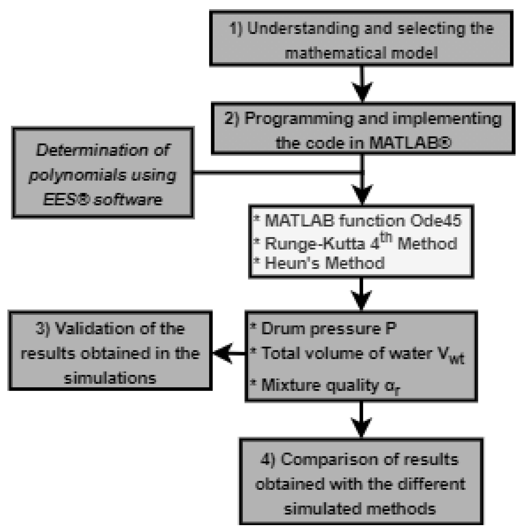
This work was developed following the methodology proposed in Figure 1. The objective is to present a systematic process for the implementation of a mathematical model that allows the dynamic simulation of the operation of a water-tube boiler. Figure 1 represents the stages in which the project was carried out, with the (*) each programmed numerical method is indicated, as well as each process variable calculated with the application of the studied methods.
2.1. Model Analysis
The study carried out by [6] has become a reference in recent years for carrying out new research on the behavior of steam generators. This work opened the way for other research studies [13,14,15]. The mathematical model proposed by [6] was studied and analyzed. The main characteristic of this model is that, despite its moderate complexity, it can easily be used to represent any drum boiler with high accuracy.
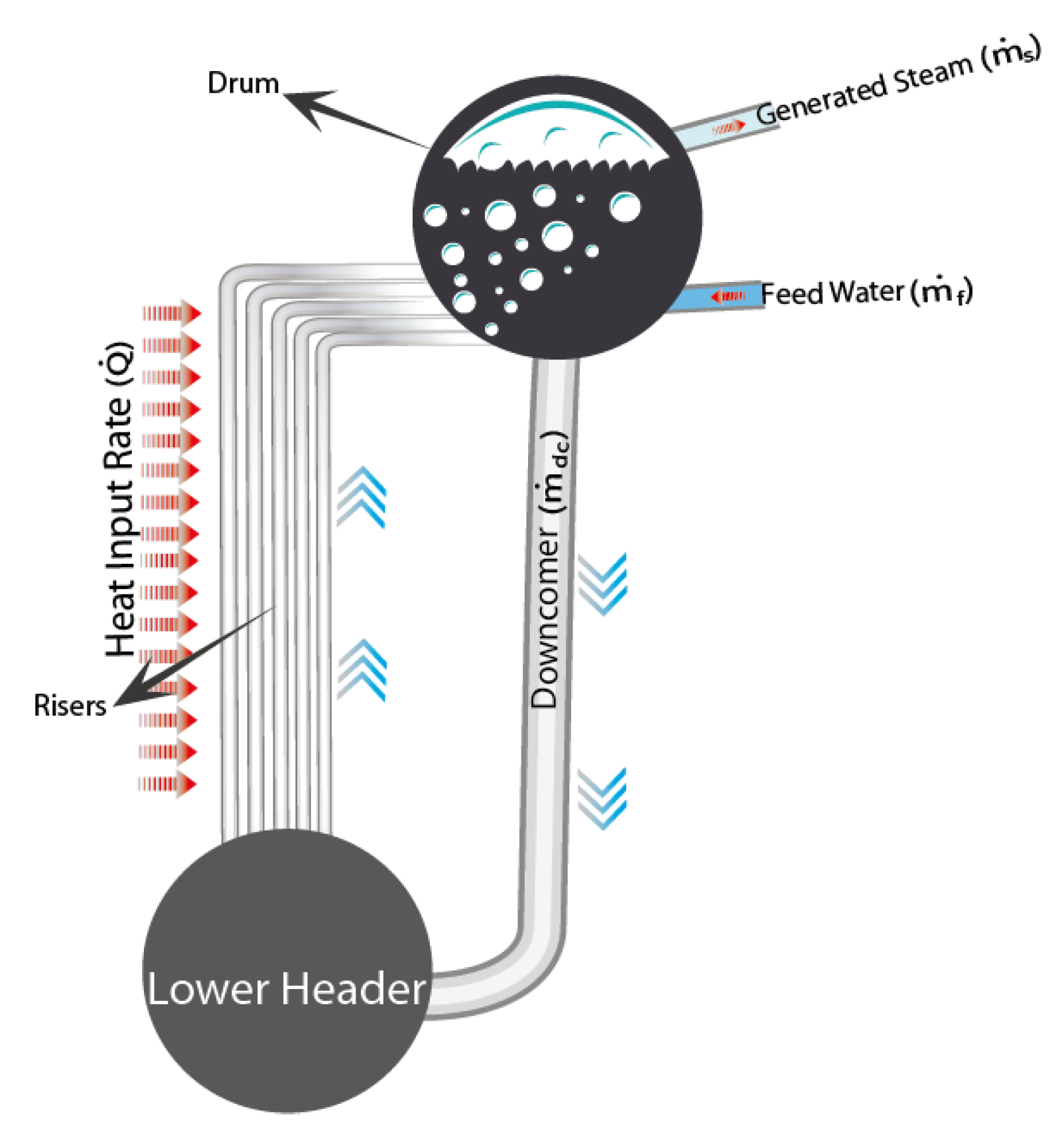
In Figure 2, the main element of a recovery boiler is detailed, Where, for its study, three main components can be highlighted: the drum, which is where the water–steam mixture is located and, in turn, has the input of the feed water and the output of generated steam , and two sections of pipeline: one that transports the water known as the down-comer , and the risers through which the water rises and begins to evaporate thanks to a heat input rate .
Equation (1) represents the overall mass balance in the drum and Equation (2), the global energy balance.
By solving the above balances, the ordinary differential Equations (3) and (4) are obtained, which describe the mathematical model in a simple way for a steam generator.
where
Equation (1) can be multiplied by and then subtracted from Equation (2). The result is shown in Equation (4) and this process results in Equation (5).
Considering that represents the enthalpy of condensation , Equation (5) is reduced to:
The dominant terms in the coefficient in Equation (6) are and . This is because the energy concentrated in the mass of water and metal are the physical phenomena of the system that determine the dynamic behavior of the pressure in the drum. As a result, can be operated as shown in Equation (7).
Riser and Down-Comer Mathematical Model
Equation (8) below allows the determination of the quality of mixture as a result of the mass and energy balance in the riser and down-comer of the steam generator.
where
The average steam volume fraction in the down-comer tube is calculated using Equation (9) determined by [6].
The volume fractions are derived depending on the drum pressure, and the quality values of the mixture are as follows:
where .
2.2. Determination of Terms Using Polynomials
The terms of Equations (3)–(8) were determined from the water steam tables as a function of saturation pressure . Engineering Equation Solver (EES®) software was used to plot enthalpy, density, and temperature of the metal in the drum wall. The latter was assumed to be equal to the steam saturation temperature . Then, the curve was adjusted using linear regression to each graph, thus obtaining a polynomial of degree n as a function of the saturation pressure .
2.3. Methods for Ordinary Differential Equation Solution
To simulate the proposed model [6] and validate the results, it is necessary to solve the ordinary differential equations through a numerical method that allows for obtaining results adjusted to the dynamic behavior of the boiler. Considering the characteristics of each method, such as complexity for the programming, precision in the results, steps for the solution, and computational cost [16,17,18], it was decided to use the Runge–Kutta method of order 4 and Heun’s method and compare the results with those obtained using the MATLAB® Ode45 function that solves this type of equation based on an explicit formula of RK 4 and RK5 [18].
2.3.1. Heun’s Method
This method is used to improve the estimation of the slope and involves the determination of two derivatives for the interval, one at the start point and one at the end point [16]. The two derivatives are averaged to obtain an improved estimate of the slope for the whole interval. Equations (10) and (11) shown below are used to solve differential equations with this method.
After having the values of and , each of the points in the plane (x, y) are determined using the following Equations (12) and (13).
Figure 3 shows the flow chart representing the code programmed for the solution of the ODE using Heun’s method.
2.3.2. Runge–Kutta 4th Order Method
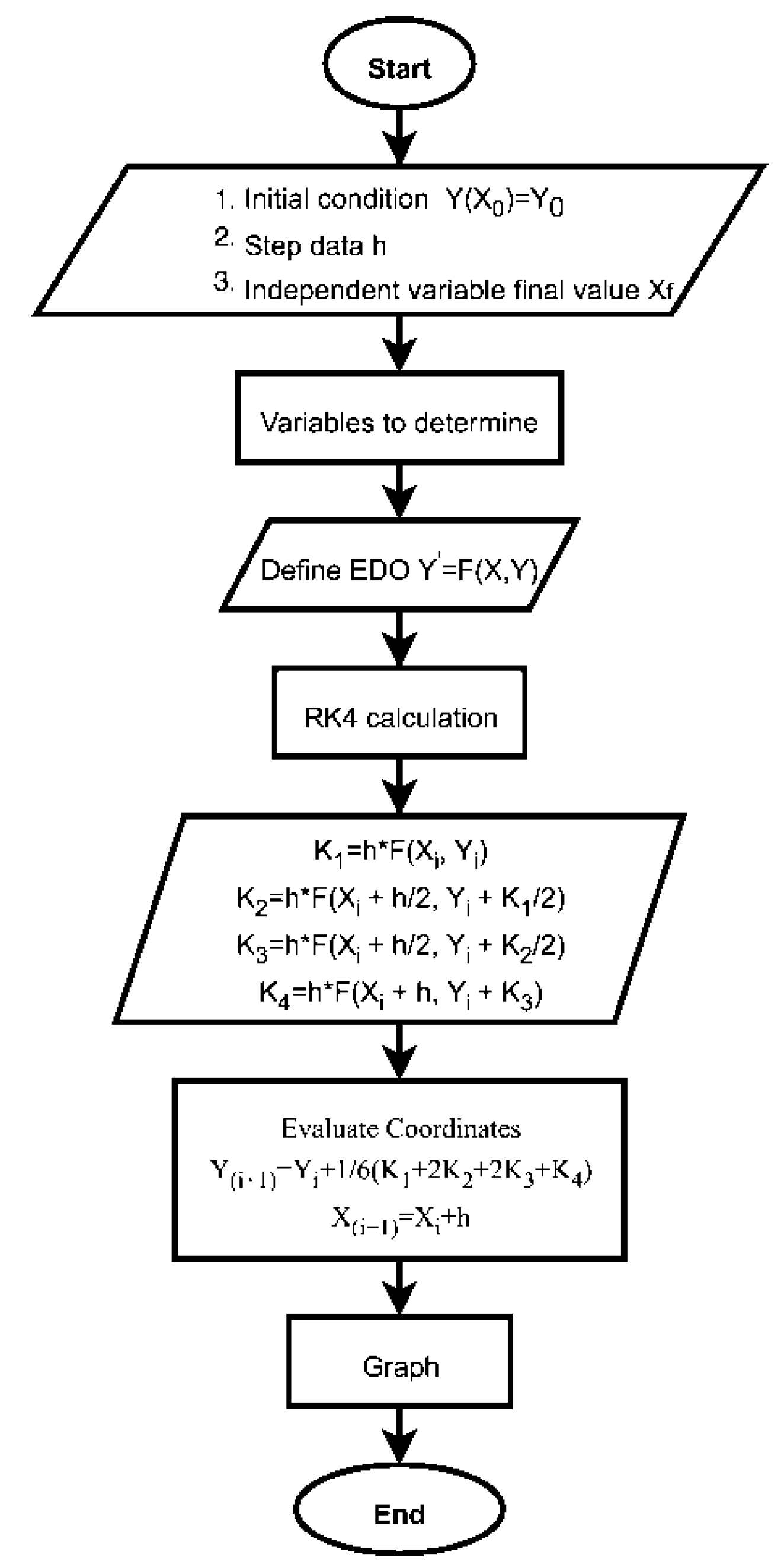
The solution of this method was programmed in MATLAB®, which develops multiple slope estimates to obtain an improved average slope for the interval. Each k represents a slope [16]. Equations (14)–(17) used by the Runge–Kutta fourth order method are shown below, where h is the step width.
When each k is obtained, the points on the (x,y) axes of the plane are determined using Equations (18) and (19), as follows:
Figure 4 shows the flow chart representing the code programmed for the solution of the ODE using the Runge–Kutta 4th order method.
2.3.3. MATLAB® Function Ode45
This method is based on an explicit formula of the Runge–Kutta (4th and 5th) order method, which is used to solve ODEs. The syntax shown in MATLAB® is:
where
- x is a matrix where each column corresponds to the dependent variables, and t is the time vector,
- odefun is the name of the function to be evaluated,
- specifies the time interval, a vector of two numbers , start and end time,
- x0 is a vector that has the initial conditions of the variables to be evaluated.
2.4. Programming and Simulation of the Model in MATLAB®
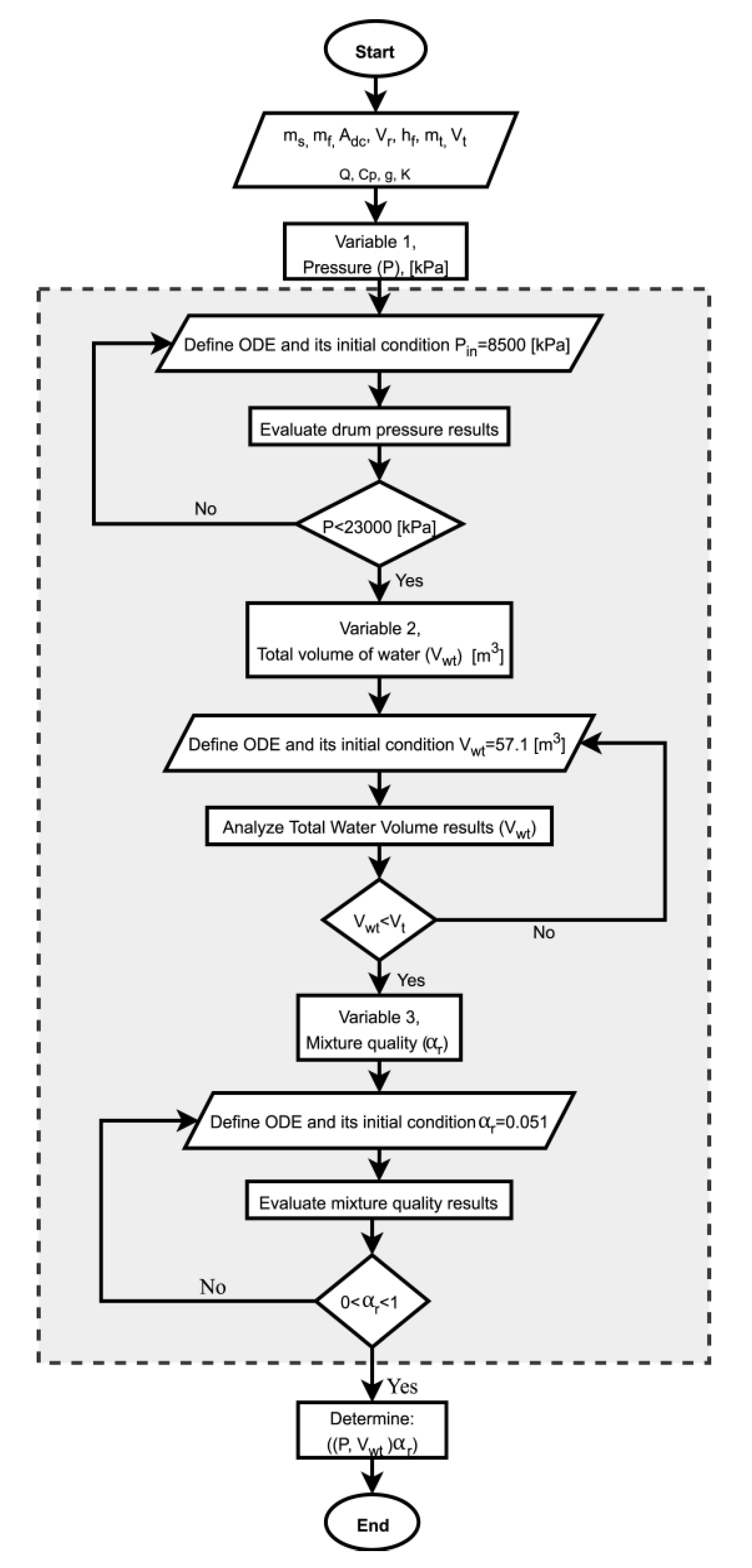
A code was developed in MATLAB® for the implementation of the mathematical model that represents by simulation the behavior of the drum pressure P, the total water volume , and mixture quality in the steam generator. Figure 5 shows the algorithm that represents the code development in MATLAB®.
2.5. Validation of Results
The data used for the simulation were taken from the P16–G16 unit operating in a power plant in Malmö, Sweden, which was reported by [6]. Table 1 shows the data used.
A time interval of 200 s was considered for the simulation of the dynamic behavior of the boiler. The percentage error was determined using Equation (20). To calculate the relative error, the reported reference value and the value obtained in the simulation are taken into account. An approximation error below 5% is acceptable when performing this type of study [19].
3. Analysis of Results
3.1. Polynomial Solution Using EES®
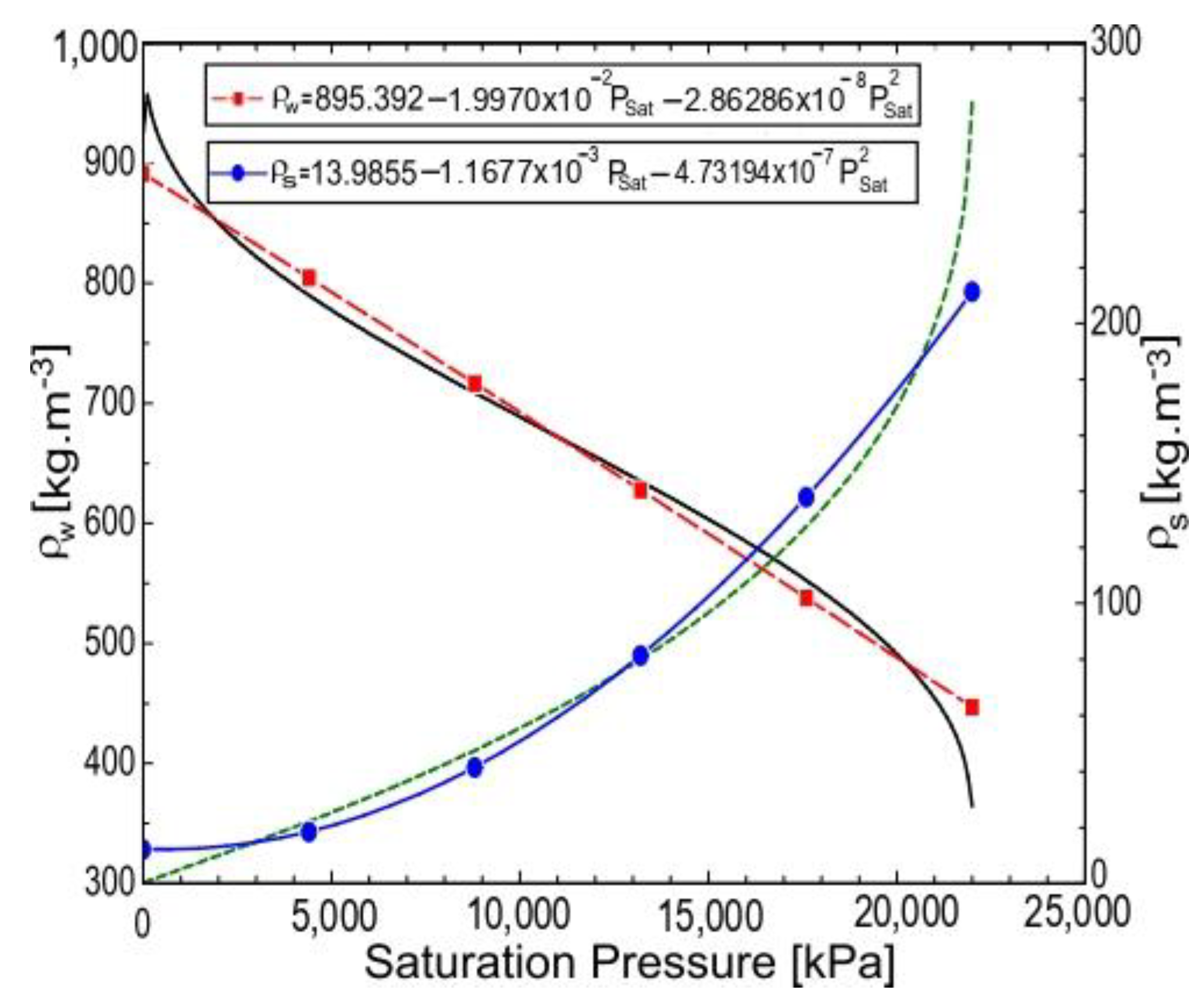
Figure 6 shows the behavior of water and steam densities as a function of saturation pressure . It is observed that when the saturation pressure increases, the saturated liquid reaches the saturated vapor point. For this reason, the density of the liquid decreases and the density of the steam increases until reaching the critical point.
Knowing this phenomenon, the curve fit is performed, resulting in the polynomials shown in the figure.
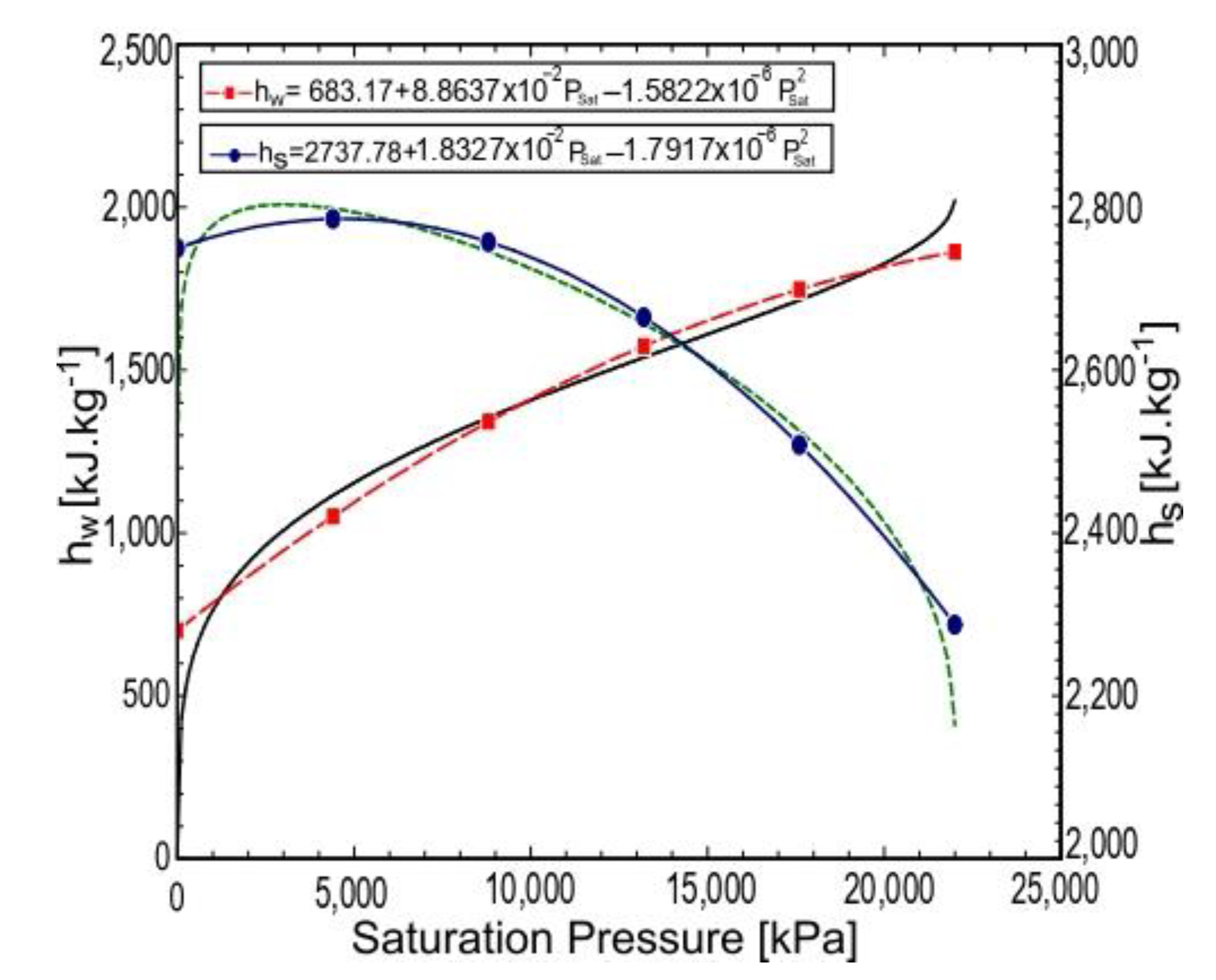
Figure 7 shows the behavior of the enthalpy of water and the enthalpy of steam as a function of the saturation pressure. It is necessary that as the saturation pressure increases, the saturated liquid reaches the saturated vapor point. For this reason, the enthalpy of water increases and the enthalpy of steam decreases until reaching the critical point.
Understanding what was done in the graph, the curve fit is performed, resulting in the polynomials shown in the figure.
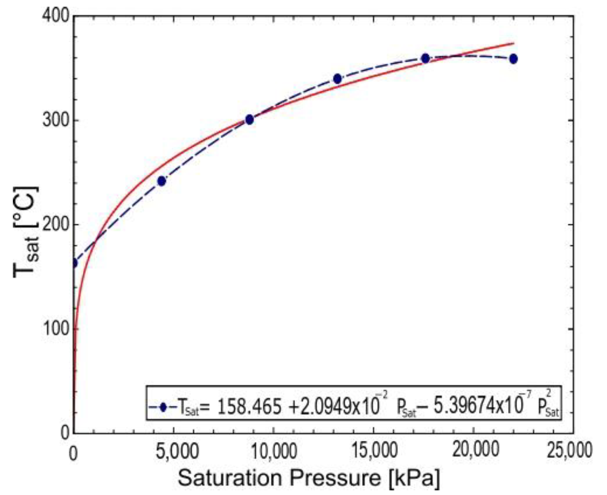
Figure 8 shows that the temperature is increasing since, as the saturation pressure increases, the temperature approaches the critical point where the critical temperature of the water is 374 °C. Knowingthis, it is assumed that the saturation temperature of the liquid is equal to the saturation temperature of the metal .
Thus, by knowingthe temperature behavior, an adjustment of the cross is made and thus we obtain the polynomial shown in the figure.
The polynomials shown in the previous figures are used to solve the differential equations that represent the behavior of the steam generator.
These polynomials apply only to the drum, since this is where there are two-phase liquid–steam conditions (mixture).
3.2. Analysis of Simulation Results
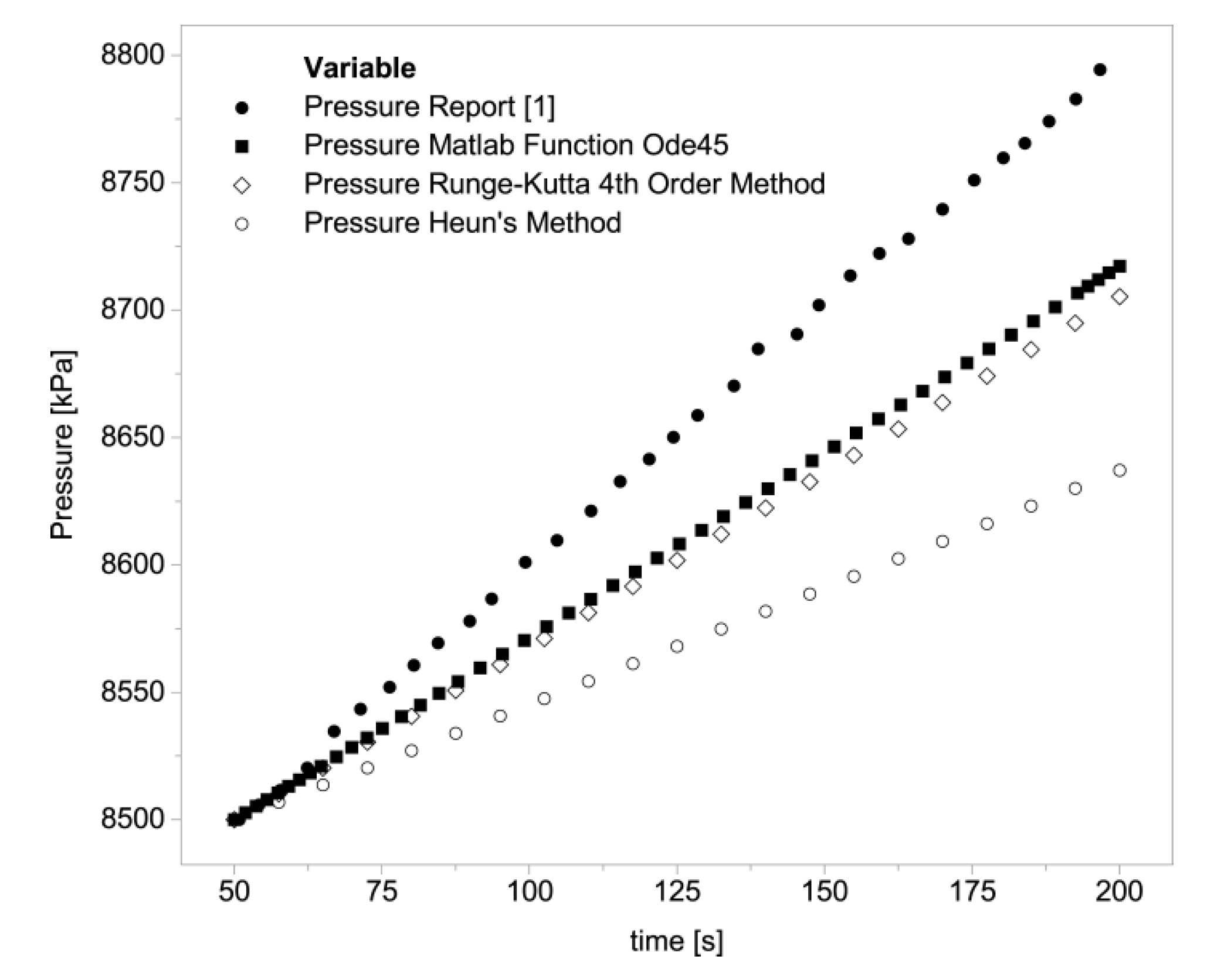
Figure 9 shows the behavior of the pressure, which is obtained using the mentioned numerical methods. These results are compared with the data shown in [6] and it is observed that the Runge–Kutta method and the Ode45 function are much closer to the data of the reported pressure graph, while the Heun’s method result is less exact.
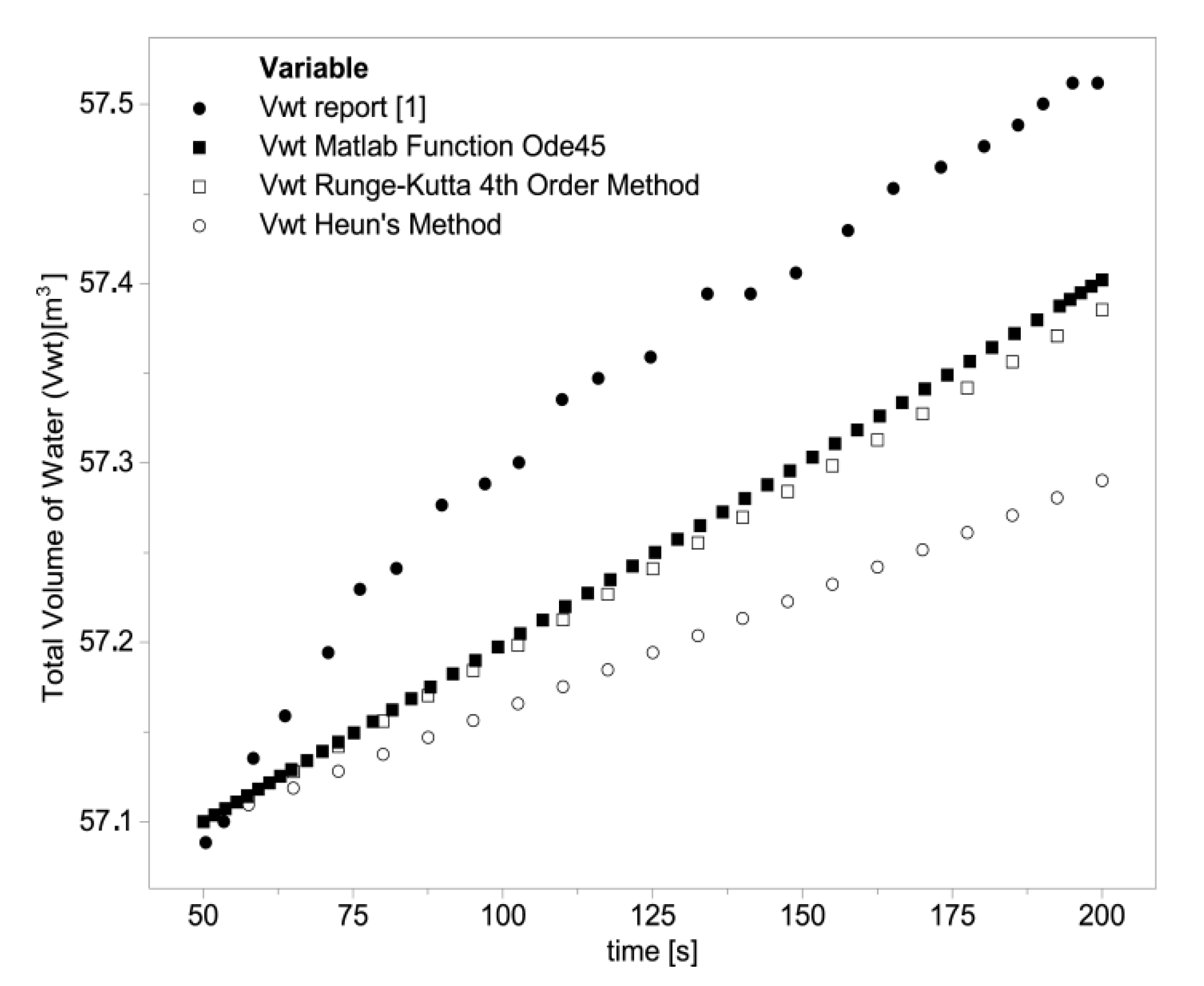
Figure 10 shows the behavior of the total volume of water obtained using the numerical methods of Runge–Kutta of the fourth order, Heun, and the Ode45 function of MATLAB®. In the figure, it can be seen that the Runge–Kutta method and the Ode45 function are the ones that would produce results close to the results reported in [6].
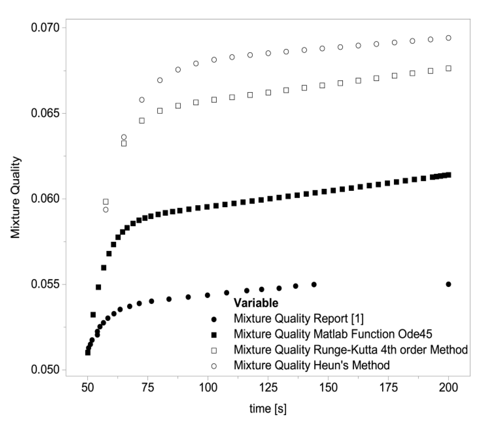
Figure 11 shows the behavior of the quality of the obtained mixture using the numerical methods of Runge–Kutta of the fourth order, Heun, and the Ode45 function of MATLAB®. The figure shows that the results of the Runge–Kutta method and Heun’s method are further from the results reported in [6], while the Ode45 function of MATLAB® is more accurate to the reported data.
3.3. Validation Using Approximation Error of the Results
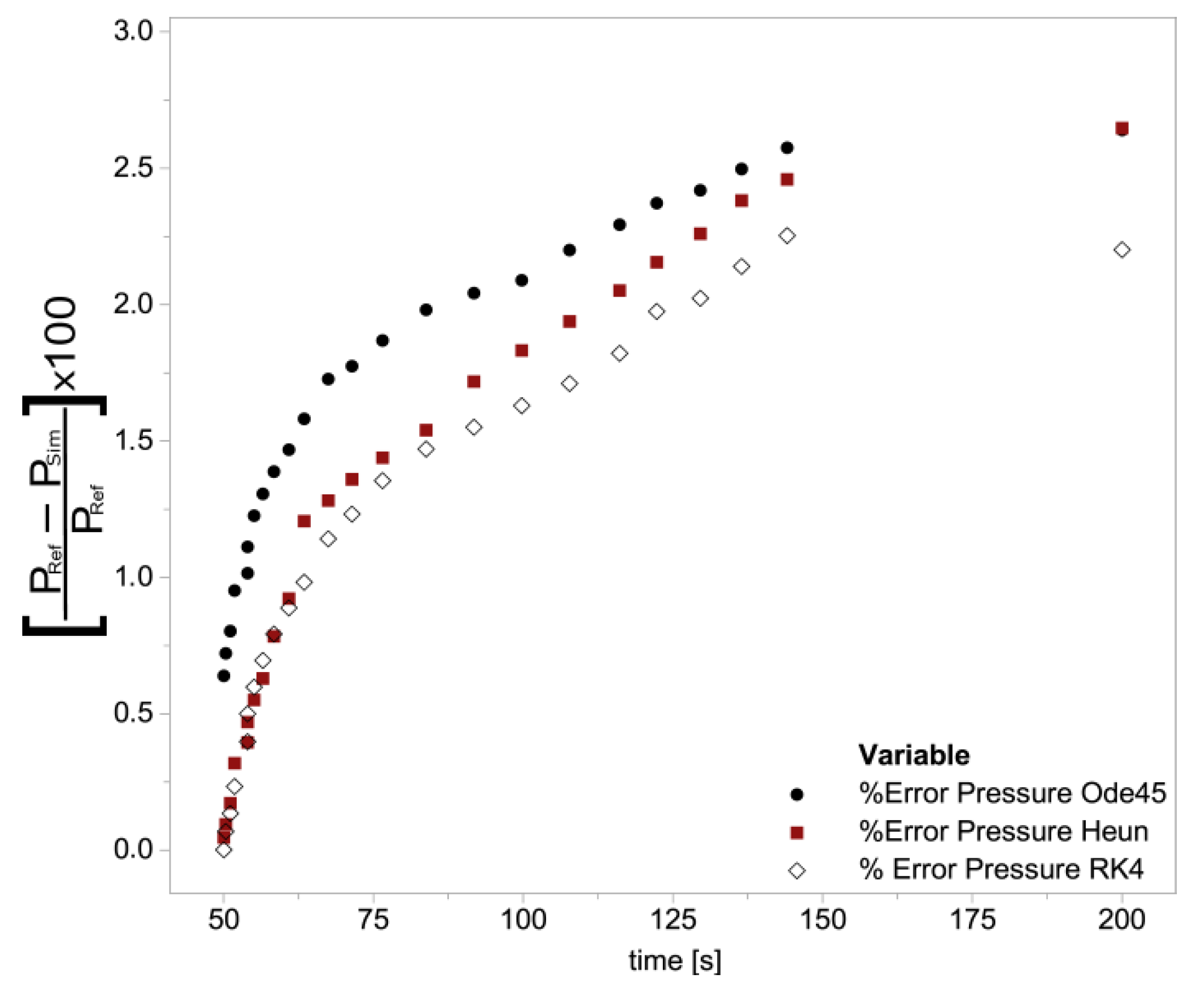
To understand the dynamic operation of the boiler, it is important to select variables to achieve the physical interpretation of the process, which describe the storage of mass, energy, and momentum in the system. The three predominant variables in the process are: the total volume of water represents the accumulation of water in the system, the pressure P in the drum represents the energy received by the system, and, finally, the quality of the mixture that represents the distribution of water–steam that represents the fraction of steam in the risers [14]. Figure 12 shows the difference between the pressure data obtained, using the different numerical methods, and the pressure reports shown in [6]. This difference in results is obtained using Equation (20) and thus determines the approximation error with each of the methods and the report [6].
When conducting this study, it can be seen that the three solution goals are in an error range between 2.2% and 2.5%.
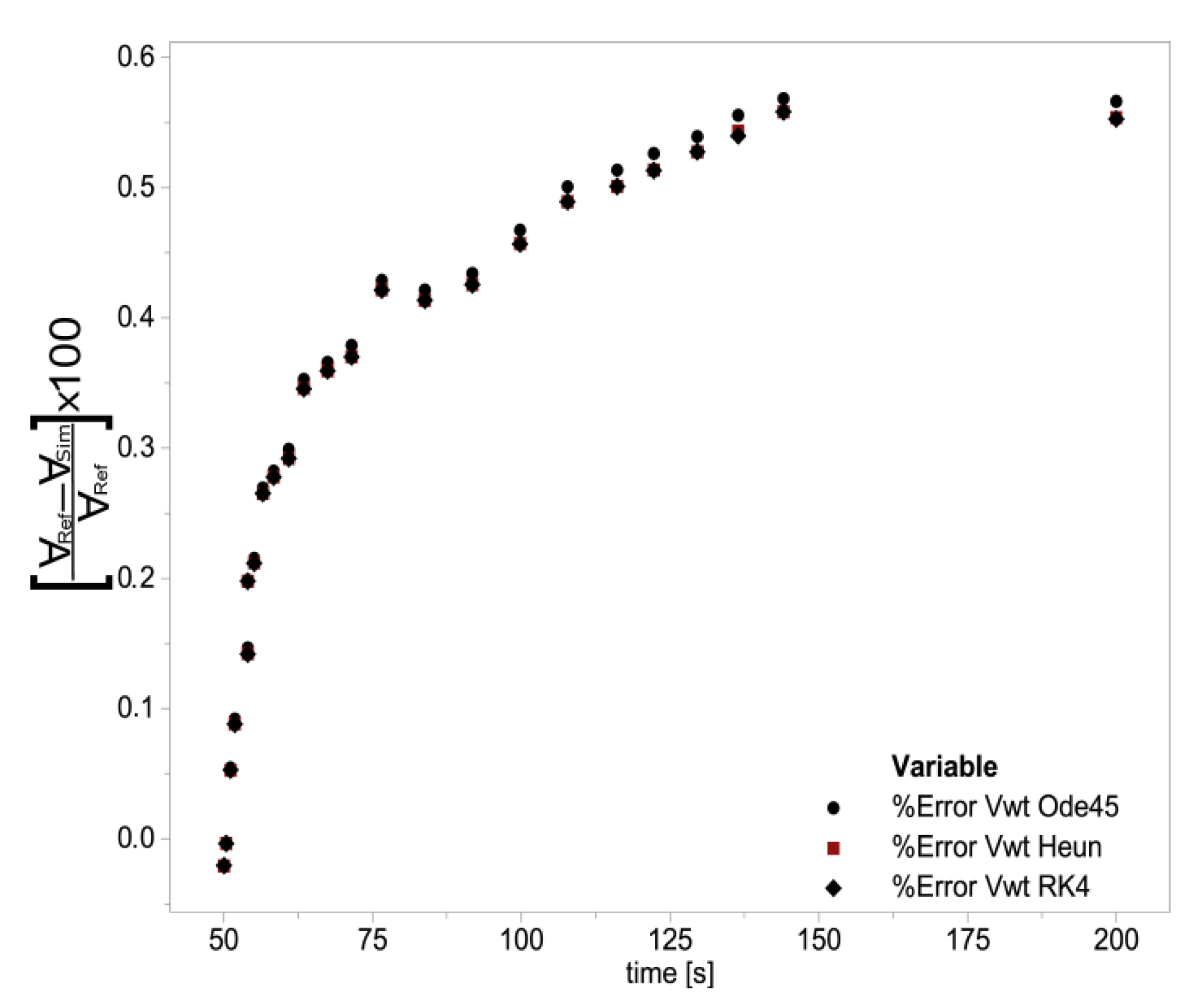
In Figure 12, it is observed that the three methods used present errors below 2.5% in the calculation of the pressure, and this indicates that they can be valid to determine this variable, however, with the RK4 method, a lower error is obtained in the results, stabilizing its value around 2%. For the pressure calculation, the highest error percentages are presented when using the Ode45 function with a maximum value of 2.5% for the simulated time. Figure 13 shows the difference between the total water volume data obtained, using the different numerical methods, and the volume reports shown in [6]. This difference in results is obtained using Equation (20) and thus determines the approximation error with each of the methods and the report [6].
Analyzing Figure 13, it can be seen that the three methods present a good behavior to determine the total volume of water with practically equal percentages of error and minimum values that are below 0.6% during the simulated operating time.
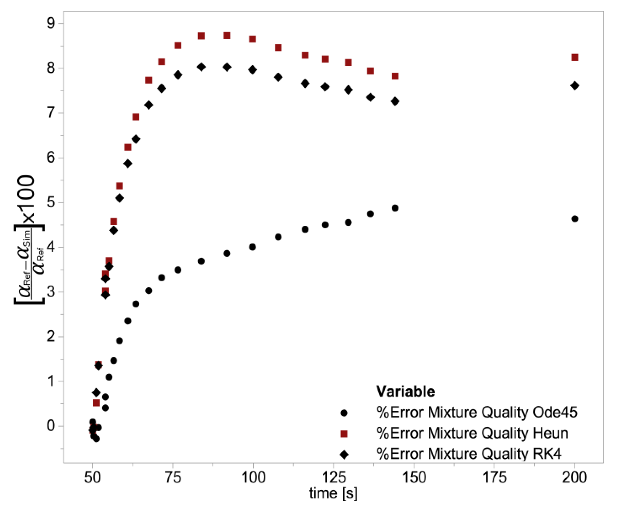
Figure 14 shows the difference between the quality data of the mixture obtained, using the different numerical methods and the quality reports shown in [6]. This difference in results is obtained using Equation (20) and thus determines the approximation error with each of the methods and the report in [6].
Figure 14 shows that for Heun’smethod and the RK4 function in the time range between 75 and 100 s, the error obtained in the calculation of the quality of the mixture tends to stabilize at a value of around 7% after an accelerated increase during the first seconds of the simulation. Undoubtedly, the Ode45 function allows for obtaining the lowest percentage of error in the calculation of the quality of the mixture, stabilizing its value around a maximum of 4.5%, much lower than those reached by RK4 and Heun’smethod of 7.5% and 8.5%, respectively.
4. Discussion
In the present work, the Runge–Kutta numerical method of order 4, Heun’s numerical method, and the MATLAB® Ode 45 function were used to reproduce experimental values of the reference [6], which simulates the behavior of pressure, total volume of water, and quality of the mix in the boiler drum. Based on the results obtained, it is valid to affirm that the three methods can be used solve the ordinary differential equation and represent in general terms the dynamic behavior of the three most important variables in the operation of the boiler, however, when analyzing the percentage of error in the results, it is evidenced that the RK4 method is the best option to represent the behavior of the pressure in the drum and the Ode4 function to determine the quality of the mix. The three methods present very good results to determine the total volume of water with minimum percentages of error that do not exceed 0.6%.
Author Contributions
The author C.Á. contributed to the conceptualization. He also programmed and validated the simulation of the applied model, supervised the execution of the project, prepared the original draft of the work, and made the adjustments based on the editing modifications. The author E.E. contributed to the conceptualization and definition of the methodology applied in the development of the work, as well as in the writing of the original draft and its subsequent revision. The author C.J.N. contributed to the programming of the code in the software, supervised the conservation of the data and validation of the model, as well as the visualization of the results obtained, and also contributed to the revision and editing of the document. All authors have read and agreed to the published version of the manuscript.
Funding
This research received no external funding.
Institutional Review Board Statement
Not applicable.
Informed Consent Statement
Not applicable.
Data Availability Statement
Not applicable.
Acknowledgments
The project was developed with the institutional support of Universidad Francisco de Paula Santander Ocaña, Colombia.
Conflicts of Interest
The authors declare no conflict of interest.
Nomenclature
| Q | Heat flux |
| Mass flow of feed water | |
| Mass flow of steam | |
| Saturated enthalpy of steam | |
| Saturated enthalpy of water | |
| Enthalpy of feed water | |
| Specific heat | |
| Raiser volume | |
| Down-comer area | |
| Total volume | |
| Total mass | |
| Gravity | |
| k | Constant |
References
- International Energy Agency IEA. The Global Authority on Energy. 2018, Volume 12, p. 8. Available online: https://www.iea.org (accessed on 10 October 2020).
- Nordell, B. Thermal pollution causes global warming. Glob. Planet. Chang. 2003, 38, 305–312. [Google Scholar] [CrossRef]
- Sunil, P.; Barve, J.; Nataraj, P. Mathematical modeling, simulation and validation of a boiler drum: Some investigations. Energy 2017, 126, 312–325. [Google Scholar] [CrossRef]
- Butler, R.M. Thermal Recovery of Oil and Bitumen; Prentice Hall: Edmonton, AB, Canada, 1991. [Google Scholar]
- Haagen, M.; Zahler, C.; Zimmermann, E.; Al-Najami, M.M.R. Solar Process Steam for Pharmaceutical Industry in Jordan. Energy Procedia 2015, 70, 621–625. [Google Scholar] [CrossRef] [Green Version]
- Aström, K.; Bell, R. Drum-boiler dynamics. Automatica 2000, 36, 363–378. [Google Scholar] [CrossRef]
- Äström, K.J.; Bell, R.D. Simple drum-boiler models. Power Syst. Model. Control Appl. 1988. [Google Scholar] [CrossRef] [Green Version]
- Adam, E.; Marchetti, J. Dynamic simulation of large boilers with natural recirculation. Comput. Chem. Eng. 1999, 23, 1031–1040. [Google Scholar] [CrossRef]
- Bhambare, K.; Miltra, S. Modeling of a Coal-Fired Natural Circulation Boiler. J. Energy Resour. Technol. 2007, 129, 159–167. [Google Scholar] [CrossRef]
- Taimoor, A.; Alghamdi, M.; Farooqi, O.; Siddiqui, M.; Zain-ul-abdein, M.; Saleem, W.; Ijaz, H.; Ali, A. Comprehensive Dynamic Modeling, Simulation, and Validation for an Industrial Boiler Incident Investigation. Process Saf. Prog. 2019, 38, e12040. [Google Scholar] [CrossRef]
- Tognoli, M.; Najafi, B.; Marchesi, R.; Rinaldi, F. Dynamic modelling, experimental validation, and thermo-economic analysis of industrial fire-tube boilers with stagnation point reverse flow combustor. Appl. Therm. Eng. 2019, 149, 1394–1407. [Google Scholar] [CrossRef]
- González, P.; Gómez, J.; Ferruzza, D.; Haglind, F.; Santana, D. Dynamic performance and stress analysis of the steam generator of parabolic trough solar power plants. Appl. Therm. Eng. 2019, 147, 804–818. [Google Scholar] [CrossRef]
- Keshavar, O.; Jafarian, A.; Shekafti, M. Dynamic simulation of a heat recovery steam generator dedicated to a brine concentration plant. J. Therm. Anal. Calorim. 2018, 135, 1763–1773. [Google Scholar] [CrossRef]
- Ahmed, S.; Elhosseini, M.; Arafat Ali, H. Modelling and practical studying of heat recovery steam generator (HRSG) drum dynamics and approach point effect on control valves. Ain Shams Eng. J. 2018, 9, 3187–3196. [Google Scholar] [CrossRef]
- Huan, L.; Weide, H. A water level dynamics simulation model of AP1000’s steam generator based on Åström-Bell model. In IOP Conference Series: Earth and Environmental Science; IOP Publishing: Bristol, UK, 2019; Volume 310. [Google Scholar] [CrossRef]
- Griffiths, D.V.; Smith, I.M. Numerical methods for engineers. In Numerical Methods for Engineers, 2nd ed.; Mcgraw-Hill: New York, NY, USA, 2006. [Google Scholar]
- Caiza, W. Métodos Numéricos; Prentice Hall: Madrid, Spain, 2015. [Google Scholar]
- MathWorks. Documentation: MATLAB. 2015. Available online: https://la.mathworks.com/ (accessed on 10 October 2020).
- Mezo, J. Encuestas y Margen de Error: Unaguíapráctica. 2015. Available online: http://www.cuadernosdeperiodistas.com/encuestas-y-margen-de-error-una-guia-practica/ (accessed on 10 October 2020).
Figure 1.
Block diagram representing the research development process.

Figure 2.
Schematic representation of the steam generator.

Figure 3.
Flow chart of Heun’s 4th order method in MATLAB®.

Figure 4.
Flow chart of the Runge–Kutta 4th order method in MATLAB®.

Figure 5.
Flow chart of the code develop in MATLAB® for the Ode solution.

Figure 6.
Graph used to determine the density polynomials of saturated liquid and saturated steam through linear regression (curve fitting) in the EES® software.
Figure 6.
Graph used to determine the density polynomials of saturated liquid and saturated steam through linear regression (curve fitting) in the EES® software.

Figure 7.
Graph used to determine the polynomials of enthalpy of water and enthalpy of steam, as a function of saturation pressure through linear regression (curve fitting) in the EES® software.
Figure 7.
Graph used to determine the polynomials of enthalpy of water and enthalpy of steam, as a function of saturation pressure through linear regression (curve fitting) in the EES® software.

Figure 8.
Graph used to determine the saturation temperature polynomial using linear regression (curve fitting) in the EES® software.
Figure 8.
Graph used to determine the saturation temperature polynomial using linear regression (curve fitting) in the EES® software.

Figure 9.
Pressure behavior with different solution methods (Ode45, Runge–Kutta, Heun).

Figure 10.
Behavior of the total volume of water with the different solution method (Ode45, Runge–Kutta, Heun).
Figure 10.
Behavior of the total volume of water with the different solution method (Ode45, Runge–Kutta, Heun).

Figure 11.
Behavior of the mixture quality with the different solution methods (Ode45, Runge–Kutta, Heun).
Figure 11.
Behavior of the mixture quality with the different solution methods (Ode45, Runge–Kutta, Heun).

Figure 12.
The approximation error for the total volume of water in the boiler with respect to the reference volume.
Figure 12.
The approximation error for the total volume of water in the boiler with respect to the reference volume.

Figure 13.
Approximation error for calculations of total water volume in the boiler.

Figure 14.
Approximation error for the quality of the mixture in the boiler.


Table 1.
Data used to perform the dynamic simulation of the steam generator.
| Operation Data | ||
|---|---|---|
| Variable | Units | Value |
| Heat flux | 86,000 | |
| Mass flow of water | 50 | |
| Mass flow of steam | 50 | |
| Specificheat | 500 | |
| Enthalpy of water | 1080.9 | |
| Raiser volume | 37 | |
| Down-comer area | 0.1123 | |
| Total volume | 88 | |
| Total mass | 300,000 | |
| Gravity | 9.81 | |
The table was recreated according to [6].
Publisher’s Note: MDPI stays neutral with regard to jurisdictional claims in published maps and institutional affiliations. |
© 2021 by the authors. Licensee MDPI, Basel, Switzerland. This article is an open access article distributed under the terms and conditions of the Creative Commons Attribution (CC BY) license (https://creativecommons.org/licenses/by/4.0/).
Share and Cite
MDPI and ACS Style
Álvarez, C.; Espinel, E.; Noriega, C.J. Study of Different Alternatives for Dynamic Simulation of a Steam Generator Using MATLAB. Fluids 2021, 6, 175. https://0-doi-org.brum.beds.ac.uk/10.3390/fluids6050175
AMA Style
Álvarez C, Espinel E, Noriega CJ. Study of Different Alternatives for Dynamic Simulation of a Steam Generator Using MATLAB. Fluids. 2021; 6(5):175. https://0-doi-org.brum.beds.ac.uk/10.3390/fluids6050175
Chicago/Turabian StyleÁlvarez, Cristhian, Edwin Espinel, and Carlos J. Noriega. 2021. "Study of Different Alternatives for Dynamic Simulation of a Steam Generator Using MATLAB" Fluids 6, no. 5: 175. https://0-doi-org.brum.beds.ac.uk/10.3390/fluids6050175