Modeling of the Effects of Pleat Packing Density and Cartridge Geometry on the Performance of Pleated Membrane Filters

Abstract

Pleated membrane filters are widely used to remove undesired impurities from a fluid in many applications. A filter membrane is sandwiched between porous support layers and then pleated and packed into an annular cylindrical cartridge with a central hollow duct for outflow. Although this arrangement offers a high surface filtration area to volume ratio, the filter performance is not as efficient as those of equivalent flat filters. In this paper, we use asymptotic methods to simplify the flow throughout the cartridge to systematically investigate how the number of pleats or pleat packing density affects the performance of the pleated membrane filters. The model is used to determine an optimal number of pleats in order to achieve a particular optimum filtration performance. Our findings show that only the “just right”—neither too few nor too many—number of pleats gives optimum performance in a pleated filter cartridge.

1. Introduction

Filtration is the process of separating contaminants from a liquid or gas by using filter membranes. There are a multitude of different applications of membrane filters, but some of the most common examples include use in the pharmaceutical industry, biotechnology, semiconductor fabrication, water treatment, food production, mask production, vacuum cleaners and air purifiers [1,2,3,4,5,6,7,8]. Filters are generally made of porous membranes, whose internal morphologies and pore geometry affect the filtration efficiency [9,10,11,12,13,14,15]. In addition, the solvent and contaminants’ properties may alter the filtration performance. In the case of solid particles, the most practical method of filtration is based on the geometry and shapes of the particles, dictating the best choice of membranes for the filtration process. As a fluid flows through membrane filters, separation of particles can occur either from blockage and/or adsorption, depending on the particle sizes. If a particle enters a pore, in which its narrowest part is smaller than the particle’s typical size, the pore will be blocked; otherwise, the particle can stick to the pore wall. Generally speaking, fouling mechanisms impede filter performance by adsorption (a collection of small particles stick to the pores’ walls and shrink them); complete blocking (pores become fully blocked by large particles); intermediate blocking (medium-sized particles block a portion of the pores’ volume); and by caking (particles at the pores’ inlets accumulate and then form a cake layer on the membrane surface), as described in [10,11,12,13,14,16,17,18]. These mechanisms of fouling add more resistance to the flow, which requires a higher pressure gradient (or more energy) for the fluid to overcome the fouling and pass through the membrane [19,20,21,22,23]. It is important to note, as also later discussed in Section 2.2, that only two mechanisms of fouling are incorporated in this paper: small particle adsorption and blocking or sieving by large particles. It should also be noted that our model does not consider swelling of the porous medium due to water absorption, as discussed in [24].

Pleated membrane filters are considered as an efficient type of filter used in a variety of industrial applications such as drinking water production, vaccine purification, and sterilization of natural gases in order to remove undesired particles from the feed solution [11,25,26,27]. The three crucial design attributes of a pleated filter are the pleat height, pleat packing density, and the pleat type [28]. The pleat height of a filter is the depth of a given pleat; the packing density represents the number of pleats filled within the volume of a cartridge; the pleat type is the pattern in which the fabrics of the filter are folded to construct the pleats. There are various pleated filter geometries and we focus on the cylindrical one in this paper [28]. Typically, in a pleated membrane filter cartridge, the membrane is placed between two supporting layers and the resulting three layers are folded (pleated) and placed into an annular cylindrical cartridge.

The design and construction of a pleated filter is an important process, since it provides a fundamental understanding of the geometry and unique structure of the pleated filter, which in turn affects the filtration performance. Pleated filter cartridges are constructed by heating the membrane to a specific temperature such that the pleats in the membrane become permanent. While this process is taking place, the pleat height and the pleat type are also configured by the manufacturer. To create a cylindrical shape: (i) the ends of the pleats are sealed together and (ii) the lengths are adjusted accordingly in order to fit the dimensions of the cartridge. The pleats can then be packed into the cylindrical housing with both inlet and outlet units to complete the pleated membrane cartridge design [28,29].

Pleated membrane filters are more compact in comparison to equal-area nonpleated (flat) membrane filters. Therefore, they have a greater surface area to volume ratio [11,30,31]; however, this can also introduce various disadvantages. As shown in previous studies [11,31], the performance of the pleated membrane filters are inferior compared to the flat (unpleated) filters with equivalent membrane surface areas. This stems from several factors, such as the additional resistance to the overall system due to the pleat packing density (PPD), as well as the support layers, the complex fluid dynamics within the pleated membrane, and possible damage of the membrane occurring during the pleating process. Multiple studies have demonstrated that membrane permeability is not the only factor that affects the overall filtration performance. Dense pleating can also cause a significant decrease in the filtration efficiency of over 50% in comparison to a flat sheet medium with similar permeability and an equivalent surface area [32,33,34]. While pleated membrane filters have a larger surface area than the flat membrane filters, a greater amount of pleats (or higher PPD) worsens the filter performance by increasing the overall system resistance. Therefore, this presents the question on how to optimize the filter cartridge geometry and the pleat packing density in such a way that the filter yields maximum performance.

Recent works [11,31] only attempted to answer part of this question (the effects of pleat geometry on the filter performance) using highly simplified models that focused only on a 2D flow through the membrane, meaning that the models did not account for any variation along the filter cartridge axial direction. However, our new quasi-3D model (the schematic shown in Figure 1a) addresses the mentioned extension by including two additional regions to make the model more realistic: (i) the empty area, where the flow enters the cartridge and then passes across the pleated membrane; (ii) the hollow region, which is a central hollow duct for outflow. In total, the empty area, the pleated membrane and the hollow region are all incorporated in our model. In this paper, we focus on the pleat packing density and the filter cartridge’s geometry as the main characteristics of a pleated membrane filter to achieve the optimal filtration performance.

The paper is first laid out in Section 2 by describing the flow through the hollow region and the empty area with the incompressible axisymmetric Stokes equations for low Reynolds numbers, while the flow in the membrane area is modeled by Darcy’s law. Each of these equations is given their respective boundary conditions based on the physical geometry. Next, we nondimensionalize the model in Section 2.1.1. In Section 2.1.2, we exploit the small aspect ratios of the filter cartridge and pleats and use asymptotic methods to simplify the system of equations. Then, we arrive at coupled boundary value problems for pressure and velocities in each of the three regions, as well as the permeability of the membrane and support layers, evolving with space and quasi-statically with time. These equations are solved numerically and presented in Section 3 to ultimately demonstrate the effects of pleat packing density and cartridge geometry on the filter performance. Finally, the discussion of the model and results are concluded in Section 4 in the context of industrial pleated membrane filters and of future modeling directions.

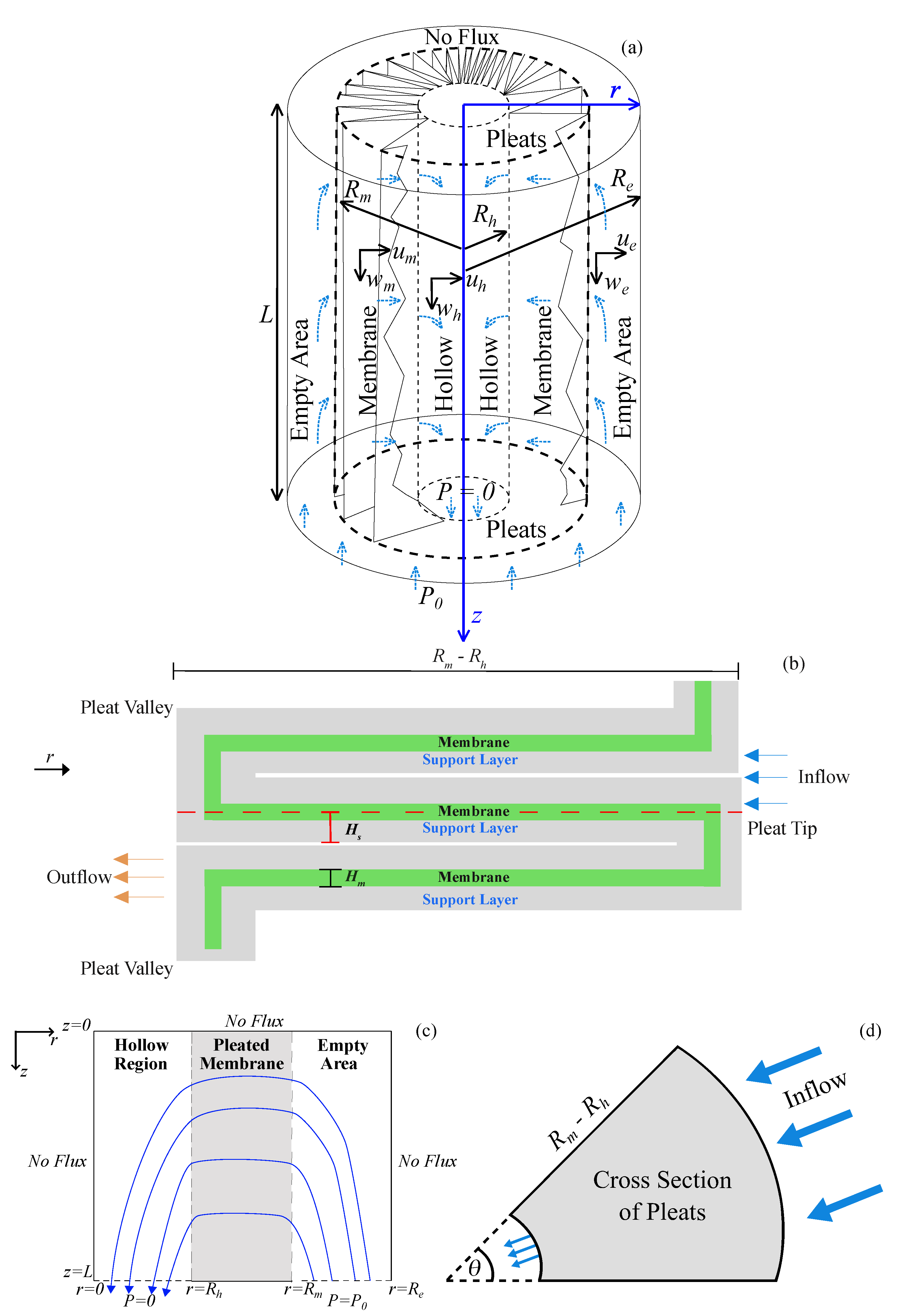
2. Mathematical Description

We consider the filtration flow problem through a pleated membrane filter cartridge consisting of a central duct surrounded by an annular pleated membrane (see Figure 1a), resulting in three different regions of the model: hollow duct, pleated membrane, and empty area. We consider the cartridge to have high pleat packing density, while assuming each pleat to be identical and part of a periodic array along the arc of the cartridge. To make the problem amenable to analytical techniques while still capturing key features of the PPD and the cartridge geometry on the filtration efficiency, we introduce an axisymmetric coordinate system, $(r,z)$. We denote the radius of the hollow region as $R_h$, the length of the pleat (from the inner to outer cartridge boundary) as $R_m-R_h$, and the total radius of the pleated filter cartridge given as $R_e$. The height of the pleated filter cartridge is denoted by L, and we assume that $R_h/L\ll 1$ and $R_m/L\ll 1$. The porous membrane consists of a membrane layer sandwiched between two support layers, as shown in Figure 1b. The membrane thickness $H_m$ and the support layer thickness $H_s$ are both assumed to be much smaller than the pleat length, $R_m-R_h$. In addition, the support layer is much thicker than the membrane, which is typical in pleated membrane filters [28,29], specifically, $H_m\ll H_s\ll R_m-R_h$ (see Figure 1b).

With specified pressure $P_0$, the solvent enters from the cartridge inlet at the bottom of the empty area, $R_m<r<R_e$, $z=L$, to flow upward, travels through the membrane $R_h<r<R_m$, $0<z<L$, and flows down the hollow region towards the outlet, $0<r<R_h$, $z=L$, where the pressure is set to 0 (see Figure 1c). It is important to note that the pressure in each of the three regions is continuous at each interface. The top of the cartridge at $z=0$, the sides of the empty area $r=R_e$, and the center of the cartridge, $r=0$ are all set to have no-flux boundary conditions. Since the geometry has symmetry along the centerline, we show only the right half of the pleated membrane filter cartridge in Figure 1c. While we do not account for angular dependency $\theta$ in our model, we introduce this angle, which sweeps across a pleat in order to derive an equation for the average of the support layers and membrane permeabilities (details of the derivation are included in Appendix A). Figure 1d shows an arbitrary cross section of the pleated membrane filter with angle $\theta$ and pleat length $R_m-R_h$.

2.1. Fluid Transport

We assume the feed is a dilute suspension of particles, which we treat as an incompressible Newtonian fluid. We denote the fluid velocity and pressure by $\mathbf{u}=(u,w)$ and p, with subscripts h, m and e denoting the hollow region, membrane and empty area, respectively. There are two time scales in our model: the first one is related to the filtration flow velocity and the second one is originated from the rate of change in pore radius due to particles deposition. Since the time scale of membrane morphology change due to particle deposition is much longer compared to that of flow velocity, we employ a quasi-static model for the flow here. We describe fluid flow in the hollow region ($0<r<R_h,0<z<L$) by the Stokes equations for an incompressible Newtonian fluid with a low Reynolds number. In axisymmetric cylindrical coordinates, the Stokes equations yield is

$$\frac{\partial p_h}{\partial r}=\mu \left[\frac{1}{r}\frac{\partial }{\partial r}\left(r\frac{\partial u_h}{\partial r}\right)+\frac{{\partial }^2{u}_h}{\partial z^2}-\frac{u_h}{r^2}\right],$$

(1)

$$\frac{\partial p_h}{\partial z}=\mu \left[\frac{1}{r}\frac{\partial }{\partial r}\left(r\frac{\partial w_h}{\partial r}\right)+\frac{{\partial }^2{w}_h}{\partial z^2}\right],$$

(2)

where $\mu$ is the viscosity of the fluid. For incompressible axisymmetric flow, it follows that the continuity equation becomes

$$\frac{1}{r}\frac{\partial }{\partial r}\left(r{u}_h\right)+\frac{\partial w_h}{\partial z}=0.$$

(3)

The pleated membrane occupies $R_h<r<R_m,0<z<L$. We model the fluid transport using Darcy’s law for the flow in porous media,

$${\mathbf{u}}_m=(u_m,w_m)=-\frac{k}{\mu }\nabla p_m,\nabla =({\partial }_r,{\partial }_z),$$

(4)

where $k(r,z)$ is the average of the support layers and membrane permeabilities. Incompressibility of the flow requires

$$\frac{1}{r}\frac{\partial }{\partial r}\left(r{u}_m\right)+\frac{\partial w_m}{\partial z}=0.$$

(5)

In the empty area ($R_m<r<R_e,0<z<L$), the fluid is also modeled using the incompressible axisymmetric Stokes equations

$$\frac{\partial p_e}{\partial r}=\mu \left[\frac{1}{r}\frac{\partial }{\partial r}\left(r\frac{\partial u_e}{\partial r}\right)+\frac{{\partial }^2{u}_e}{\partial z^2}-\frac{u_e}{r^2}\right],$$

(6)

$$\frac{\partial p_e}{\partial z}=\mu \left[\frac{1}{r}\frac{\partial }{\partial r}\left(r\frac{\partial w_e}{\partial r}\right)+\frac{{\partial }^2{w}_e}{\partial z^2}\right],$$

(7)

$$\frac{1}{r}\frac{\partial }{\partial r}\left(r{u}_e\right)+\frac{\partial w_e}{\partial z}=0.$$

(8)

We assume the flow is driven by an imposed pressure difference, $P_0$, at the inlet $z=L$ in the empty area $(R_m<r<R_e)$ and exits the filter through the outlet at $z=L$ in the hollow region $(0<r<R_h)$,

$$p_e=P_0,p_h=0\mathrm{at}z=L,$$

(9)

with the symmetry conditions in the hollow region

$$u_h=0,\frac{\partial w_h}{\partial r}=0\mathrm{at}r=0.$$

(10)

The housing boundaries $z=0$ and $r=R_e$ are solid boundaries on which we impose no flux; therefore,

$$\begin{array}{c}{u}_h=w_h=u_m=w_m=u_e=w_e=0\mathrm{at}z=0,\\ u_e=w_e=0\mathrm{at}r=R_e.\end{array}$$

(11)

At the interface between the hollow region and membrane, we impose continuity of pressure and velocity,

$$p_h=p_m,u_h=\varphi u_m\mathrm{at}r=R_h,$$

(12)

where $\varphi$ is the local pleated membrane porosity [35] (assumed constant). Similarly, at the interface between the membrane and empty area, we impose continuity of pressure and velocity,

$$p_e=p_m,u_e=\varphi u_m\mathrm{at}r=R_m.$$

(13)

The last boundary condition represents a nonvanishing tangential slip velocity [35,36]

$$\begin{array}{c}\frac{\partial w_h}{\partial r}=-\frac{\alpha }{\sqrt{k(r,z)}}(w_h-w_m)\mathrm{at}r=R_h,\\ \frac{\partial w_e}{\partial r}=-\frac{\alpha }{\sqrt{k(r,z)}}(w_e-w_m)\mathrm{at}r=R_m,\end{array}$$

(14)

where $\alpha$ is a dimensionless slip constant that depends on the surface properties. The flux q through the filter boundary at $z=L$ is defined by

$$q={\int }_0^{R_h}2\pi r\left|\right|{\mathbf{u}}_h\left|\right|{|}_{z=L}dr={\int }_0^{R_h}2\pi r\sqrt{u_h^2+w_h^2}{|}_{z=L}dr.$$

(15)

2.1.1. Nondimensionalization

Motivated by the small aspect ratio of the pleated filter cartridge, i.e., $ϵ=R_m/L\ll 1$, we introduce dimensionless variables as follows, using hats to denote dimensionless variables:

$$\begin{array}{c}(r,z)=L(ϵ\widehat{r},\widehat{z}),(p_h,p_m,p_e)=P_0({\widehat{p}}_h,{\widehat{p}}_m,{\widehat{p}}_e),\\ (u_h,w_h)=\frac{L{P}_0{ϵ}^2}{\mu }(ϵ{\widehat{u}}_h,{\widehat{w}}_h),(u_m,w_m)=\frac{K_{}{P}_0}{R_m\mu }({\widehat{u}}_m,{\widehat{w}}_m),\\ \varphi =\frac{L^2{ϵ}^4}{K_{}}\widehat{\varphi },(u_e,w_e)=\frac{L{P}_0{ϵ}^2}{\mu }(ϵ{\widehat{u}}_e,{\widehat{w}}_e),\\ k(r,z)=K_{}\widehat{k}(\widehat{r},\widehat{z}),q=\frac{2\pi P_0{R}_m^4}{L\mu }\widehat{q},\end{array}$$

(16)

where K is the average of the support layers and the membrane permeabilities. We define the parameter $l=R_h/R_m$, which characterizes the dimensionless ratio of the inner to the outer radii of the pleated membrane, and we scale the radius of the external housing $R_e=R_m(1+{ϵ}^{*})$, where ${ϵ}^{*}\ll 1$. Dropping hats, (1)–(3) give the dimensionless system of equations in the hollow region ($0<r<l,0<z<1$)

$$\frac{\partial p_h}{\partial r}={ϵ}^2\frac{1}{r}\frac{\partial }{\partial r}\left(r\frac{\partial u_h}{\partial r}\right)+{ϵ}^4\frac{{\partial }^2{u}_h}{\partial z^2}-{ϵ}^2\frac{u_h}{r^2},$$

(17)

$$\frac{\partial p_h}{\partial z}=\frac{1}{r}\frac{\partial }{\partial r}\left(r\frac{\partial w_h}{\partial r}\right)+{ϵ}^2\frac{{\partial }^2{w}_h}{\partial z^2},$$

(18)

$$\frac{1}{r}\frac{\partial }{\partial r}\left(r{u}_h\right)+\frac{\partial w_h}{\partial z}=0.$$

(19)

Similarly, the porous membrane Equations (4) and (5) become ($l<r<1,0<z<1$)

$$u_m=-k(r,z)\frac{\partial p_m}{\partial r},$$

(20)

$$w_m=-ϵk(r,z)\frac{\partial p_m}{\partial z},$$

(21)

$$\frac{1}{r}\frac{\partial }{\partial r}\left(r{u}_m\right)+ϵ\frac{\partial w_m}{\partial z}=0.$$

(22)

In the empty area ($1<r<1+{ϵ}^{*},0<z<1$), the dimensionless equations,

$$\frac{\partial p_e}{\partial r}={ϵ}^2\frac{1}{r}\frac{\partial }{\partial r}\left(r\frac{\partial u_e}{\partial r}\right)+{ϵ}^4\frac{{\partial }^2{u}_e}{\partial z^2}-{ϵ}^2\frac{u_e}{r^2},$$

(23)

$$\frac{\partial p_e}{\partial z}=\frac{1}{r}\frac{\partial }{\partial r}\left(r\frac{\partial w_e}{\partial r}\right)+{ϵ}^2\frac{{\partial }^2{w}_e}{\partial z^2},$$

(24)

$$\frac{1}{r}\frac{\partial }{\partial r}\left(r{u}_e\right)+\frac{\partial w_e}{\partial z}=0,$$

(25)

are obtained from (6)–(8). The boundary conditions (9)–(14) give the pressure drop boundary conditions that drive the flow

$$p_e=1,p_h=0\mathrm{at}z=1;$$

(26)

the boundary conditions on the hollow region centerline

$$u_h=0,\frac{\partial w_h}{\partial r}=0\mathrm{at}r=0;$$

(27)

on the housing boundaries

$$\begin{array}{c}{u}_h=w_h=u_m=w_m=u_e=w_e=0\mathrm{at}z=0,\\ u_e=w_e=0\mathrm{at}r=1+{ϵ}^{*};\end{array}$$

(28)

at the interface between the hollow region and membrane

$$p_h=p_m,u_h=\varphi u_m\mathrm{at}r=l;$$

(29)

at the interface between the membrane and the empty area

$$p_e=p_m,u_e=\varphi u_m,w_h=0\mathrm{at}r=1;$$

(30)

and finally

$$\begin{array}{c}\frac{\partial w_h}{\partial r}=-\frac{ϵ{\alpha }_0}{\sqrt{k}}\left(w_h-\frac{ϵ}{{\varphi }_0}{w}_m\right)\mathrm{at}r=l,\\ \frac{\partial w_e}{\partial r}=-\frac{ϵ{\alpha }_0}{\sqrt{k}}\left(w_e-\frac{ϵ}{{\varphi }_0}{w}_m\right)\mathrm{at}r=1,\end{array}$$

(31)

where ${\alpha }_0=L\alpha /\sqrt{K}$ and ${\varphi }_0=\left(L^2{ϵ}^4\right)/K$. Note that we assume ${\alpha }_0=\mathcal{O}(1/{ϵ}^2)$ to be able to simplify the boundary conditions (31). The total dimensionless flux q is given by

$$q={\int }_0^{l}r\sqrt{{ϵ}^2{u}_h^2+w_h^2}{|}_{z=1}dr.$$

(32)

2.1.2. Asymptotic Analysis for the Flow

We use asymptotic analysis to derive a reduced system of governing equations at the leading order. We begin by expanding each dependent variable as an asymptotic series in power of $ϵ$ as follows. For example, we let $p_h=p_h^0+ϵp_h^1+{ϵ}^2{p}_h^2+\cdots$ and similarly expand the pressures $p_m,p_e$; the velocities $u_h,w_h,u_m,w_m,u_e,w_e$; the membrane porosity $\varphi$ and the membrane permeability k. At the leading order (omitting the superscript 0 for brevity), the Equations (17)–(31) for the hollow region, membrane and the empty area are reduced to

$$\begin{array}{c}\frac{\partial p_h}{\partial r}=0,\frac{\partial p_h}{\partial z}=\frac{1}{r}\frac{\partial }{\partial r}\left(r\frac{\partial w_h}{\partial r}\right),\\ \frac{1}{r}\frac{\partial }{\partial r}\left(r{u}_h\right)+\frac{\partial w_h}{\partial z}=0,0<r<l,0<z<1,\end{array}$$

(33)

$$\begin{array}{c}{u}_m=-k\frac{\partial p_m}{\partial r},w_m=0,\\ \frac{\partial }{\partial r}\left(r{u}_m\right)=0,l<r<1,0<z<1,\end{array}$$

(34)

$$\begin{array}{c}\frac{\partial p_e}{\partial r}=0,\frac{\partial p_e}{\partial z}=\frac{1}{r}\frac{\partial }{\partial r}\left(r\frac{\partial w_e}{\partial r}\right),\\ \frac{1}{r}\frac{\partial }{\partial r}\left(r{u}_e\right)+\frac{\partial w_e}{\partial z}=0,\\ 1<r<1+{ϵ}^{*},0<z<1,\end{array}$$

(35)

$$p_e=1,p_h=0\mathrm{at}z=1,$$

(36)

$$u_h=0,\frac{\partial w_h}{\partial r}=0\mathrm{at}r=0,$$

(37)

$$u_h=w_h=u_m=w_m=u_e=w_e=0\mathrm{at}z=0,$$

(38)

$$u_e=w_e=0\mathrm{at}r=1+{ϵ}^{*},$$

(39)

$$p_h=p_m,u_h=\varphi u_m,w_h=0\mathrm{at}r=l,$$

(40)

$$p_e=p_m,u_e=\varphi u_m,w_e=0\mathrm{at}r=1,$$

(41)

where the hollow region pressure $p_h\left(z\right)$ and empty area pressure $p_e\left(z\right)$ only vary axially, obtained from (33) and (35), respectively. Note that we use the assumption ${\alpha }_0=\mathcal{O}(1/{ϵ}^2)$ to obtain the boundary conditions in (40) and (41) for the axial velocity in the hollow region and the empty area $w_h$ and $w_e$, respectively. Integrating (33) and using boundary conditions (37) and (40) give the hollow region velocities $u_h$ and $w_h$ in terms of the hollow region pressure gradient as

$$\begin{array}{c}{u}_h(r,z)=\frac{r}{16}(2l^2-r^2)\frac{d^2{p}_h}{d{z}^2},\\ w_h(r,z)=-\frac{1}{4}\left(l^2-r^2\right)\frac{d{p}_h}{dz}.\end{array}$$

(42)

Similarly, by integrating (35) and applying boundary conditions (39) and (41), we obtain the following equations for the empty area velocities $u_e$ and $w_e$ in terms of the empty area pressure gradient

$$\begin{array}{c}{u}_e(r,z)=-\frac{1}{16}M\left(r\right)\frac{d^2{p}_e}{d{z}^2},\\ w_e(r,z)=\frac{1}{4}\left(r^2-1+\gamma lnr\right)\frac{d{p}_e}{dz},\end{array}$$

(43)

where

$$\begin{array}{c}\hfill \gamma =\frac{1-{(1+{ϵ}^{*})}^2}{ln(1+{ϵ}^{*})},M\left(r\right)=r\left(r^2-2+\gamma (2lnr-1)\right)-\\ \hfill {\displaystyle \frac{{(1+{ϵ}^{*})}^2}{r}}\left({(1+{ϵ}^{*})}^2-2+\gamma (2ln(1+{ϵ}^{*})-1)\right).\end{array}$$

(44)

Furthermore, using the boundary conditions (40) and (41) along with integrating of (34) yield the velocity $u_m$ and the $p_m$ in the membrane:

$$\begin{array}{c}{u}_m(r,z)=\frac{{\tilde{u}}_m\left(z\right)}{r},\\ p_m(r,z)=p_e\left(z\right)+{\tilde{u}}_m\left(z\right){\int }_r^1\frac{d{r}^{\prime }}{r^{\prime }k(r^{\prime },z)},\end{array}$$

(45)

where

$${\tilde{u}}_m\left(z\right)=(p_h\left(z\right)-p_e\left(z\right)){\left({\int }_l^1\frac{d{r}^{\prime }}{r^{\prime }k(r^{\prime },z)}\right)}^{-1},$$

(46)

is determined as part of the solution to the reduced model. At this stage, we now emphasize each quantity that depends on space and/or time. Combining (40), (41), (42), (43), (45) and (46) gives the resulting simplified model for $p_h(z,t)$ as

$$\frac{l^4}{16}\left({\int }_l^1\frac{d{r}^{\prime }}{r^{\prime }k(r^{\prime },z,t)}\right)\frac{{\partial }^2{p}_h(z,t)}{\partial z^2}-\varphi p_h(z,t)=-\varphi p_e(z,t),$$

(47)

$$\begin{array}{c}\hfill \frac{M\left(1\right)}{16}\left({\int }_l^1\frac{d{r}^{\prime }}{r^{\prime }k(r^{\prime },z,t)}\right)\frac{{\partial }^2{p}_e(z,t)}{\partial z^2}-\varphi p_e(z,t)=-\varphi p_h(z,t),\end{array}$$

(48)

subject to boundary conditions

$$\frac{\partial p_h}{\partial z}(0,t)=0,p_h(1,t)=0.$$

(49)

$$\frac{\partial p_e}{\partial z}(0,t)=0,p_e(1,t)=1,$$

(50)

obtained by (36), (38), (42) and (43). By adding (47) and (48) together, then integrating and using boundary conditions (49) and (50), the coupled system can be simplified further

$$p_e(z,t)=1-{\displaystyle \frac{l^4}{M\left(1\right)}}{p}_h,$$

(51)

$$\begin{array}{c}\frac{l^4}{16}\left({\int }_l^1\frac{d{r}^{\prime }}{r^{\prime }k(r^{\prime },z,t)}\right)\frac{{\partial }^2{p}_h(z,t)}{\partial z^2}-\left(1+{\displaystyle \frac{l^4}{M\left(1\right)}}\right)\varphi p_h(z,t)=-\varphi ,\\ \frac{\partial p_h}{\partial z}(0,t)=p_h(1,t)=0.\end{array}$$

(52)

Note that, after solving (52), we can obtain the velocities and pressures in all three regions using (42)–(46). In addition, the total dimensionless flux of fluid flowing across the filter outlet, introduced in (32), becomes

$$q={\int }_0^{l}r{w}_h{|}_{z=1}dr,$$

(53)

where $w_h$ can be obtained from (42) and (52).

2.1.3. Fluid Velocity and Streamfunction

For purpose of illustration, we show the visualization of the fluid flow through the membrane and the hollow region. Recall that the flow in our model is two-dimensional (axisymmetric assumption) and quasi-static; therefore, we employ streamfunction ${\psi }_m$ and ${\psi }_h$ in the membrane and the hollow region, respectively,

$$\begin{array}{c}{u}_i(r,z)=-\frac{1}{r}\frac{\partial {\psi }_i}{\partial z},w_i(r,z)=\frac{1}{r}\frac{\partial {\psi }_i}{\partial r},i\in \{m,h\}.\end{array}$$

(54)

Using the flow velocities for the membrane and the hollow region, (42) and (45), respectively, along with (54), give us the streamfunctions in these two regions as

$$\begin{array}{c}{\psi }_h(r,z)=\frac{1}{4}\left(l^2\frac{r^2}{2}-\frac{r^4}{4}\right)\frac{d{p}_h}{dz},\\ {\psi }_m\left(z\right)=-{\int }_0^z\frac{p_h\left(z^{\prime }\right)-p_e\left(z^{\prime }\right)}{{\int }_l^1\frac{d{r}^{\prime }}{r^{\prime }k(r^{\prime },z)}}d{z}^{\prime }.\end{array}$$

(55)

2.2. Membrane Fouling

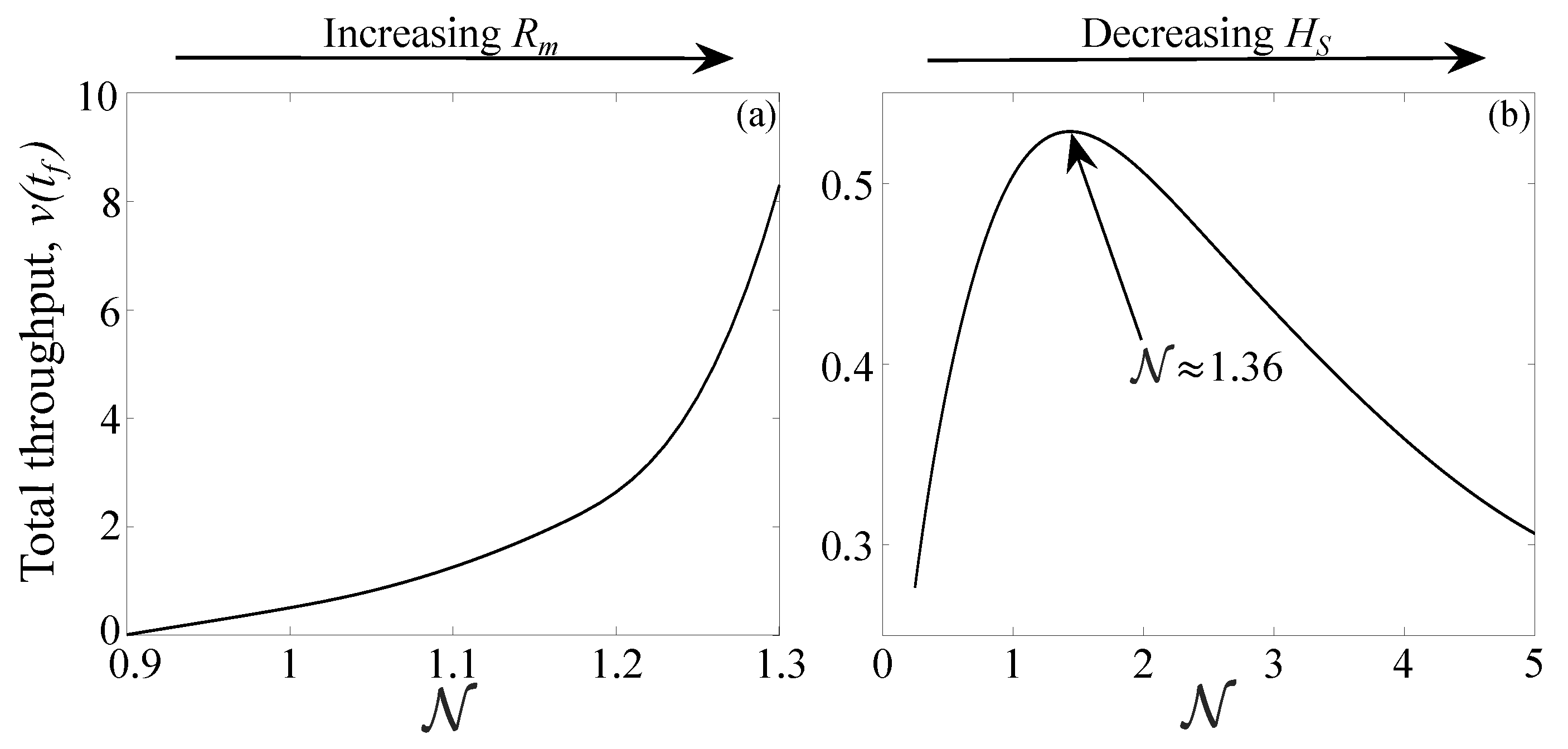
In general, the average of the support layer and membrane permeabilities $k(r,z,t)$ varies in both space and time as membrane fouling occurs. For a given average permeability $k(r,z,t)$, the boundary value problem (52) is solved to determine the velocities in both the hollow region and the membrane, as explained earlier. To close the model, we need an equation for the time evolution of the average permeability due to membrane fouling. Here, we present just the average permeability estimate (the derivation is provided in Appendix A),

$$k(r,z,t)\sim \frac{\mathcal{N}{k}_m(r,z,t)k_s(r,z)}{{\mathcal{N}}^2{k}_m(r,z,t)+k_s(r,z)},\mathcal{N}=\frac{\pi (R_m+R_h)}{H_s},$$

(56)

where $k_s(r,z)$ is the average permeability in the support layers, $k_m(r,z,t)$ is the permeability in the membrane and $\mathcal{N}$ is a dimensionless measure of packing density, which we call the packing density factor. Note that we assume the average permeability of the support layers $k_s(r,z)$ is not a function of time, since fouling does not happen in the support layers.

To derive an asymptotic model for membrane fouling with variations along the z direction, we modify the model described in Sanaei et al. [31] by introducing nonzero z-dependent pressure at the end the membrane. The membrane permeability $k_m$ varies quasi-statically and is expressed as a function of the pore radius $a(z,t)$ and the number of unblocked pores per unit area $n(r,z,t)$. The model assumes that membrane pores are long, thin cylindrical tubes, spanning the membrane, which initially all have the same radius. A more sophisticated model would allow for nonuniform shrinkage of pores due to the adsorption, but in our simple model we assume uniform adsorption so that the pore radius does not vary spatially. The time evolution of the membrane permeability induces time variation for the pressure in the support layer $p_s$. Here, we just present the final reduced model with modifications to account for the axial-dependence pressure at the interface between the membrane and the hollow region, and refer the readers to Sanaei et al. [31] for more details. The full dimensionless system is

$$\begin{array}{c}a(z,t)=1-\beta t,\\ k_m(r,z,t)=a{(z,t)}^4\left(n(r,z,t)+\frac{1-n(r,z,t)}{1+{\rho }_{b}a{(z,t)}^4}\right),\end{array}$$

(57)

$$\begin{array}{c}\frac{\partial n(r,z,t)}{\partial t}=-n(r,z,t)a{(z,t)}^4{e}^{-ba(z,t)}\\ \left(2p_s(r,z,t)+c_1(z,t){\int }_r^1\frac{d{r}^{\prime }}{k_s(r^{\prime },z)}+c_2(z,t)\right),\end{array}$$

(58)

$$\begin{array}{c}\frac{\partial }{\partial r}\left(k_s(r,z)\frac{\partial p_s(r,z,t)}{\partial r}\right)-2\Gamma k_m(r,z,t)p_s(r,z,t)=\\ \Gamma k_m(r,z,t)\left(c_1(z,t){\int }_r^1\frac{d{r}^{\prime }}{k_s(r^{\prime },z)}+c_2(z,t)\right),\end{array}$$

(59)

subject to conditions

$$n(r,z,0)=1,$$

(60)

$$p_s(1,z,t)=p_e(z,t),\frac{\partial p_s}{\partial r}(1,z,t)=\frac{c_1(z,t)}{k_s(1,z)},$$

(61)

$$\begin{array}{c}{p}_s(l,z,t)=-\left(c_1(z,t){\int }_0^1\frac{d{r}^{\prime }}{k_s(z,r^{\prime })}+c_2(z,t)+p_h(z,t)\right),\\ \frac{\partial p_s}{\partial r}(l,z,t)=0,\end{array}$$

(62)

where $p_s$ is the pressure in the support layer, $\beta =\left(8\mu E{H}_m\right)/\left(\pi a_0^4{P}_0{g}_{\infty }\right)$ is the dimensionless pore shrinkage rate representing the time scale in which pores close due to adsorption, relative to that in which particles block individual pores from upstream, $g_{\infty }$ is the total large particle concentration and E is the rate of pore radius shrinkage. $\Gamma =K_{m0}{(R_m-R_h)}^2/\left(K_s{H}_m{H}_s\right)$ is a dimensionless measure of the relative importance of the resistance of the packing material to that of the membrane, b is the ratio of initial pore size to characteristic particle size and ${\rho }_b$ is the dimensionless parameter that characterizes blocking strength.

3. Results

The model consists of various dimensional and dimensionless parameters shown in

Table 1. Dimensional parameter values [11,28,31,37,38,39].

Parameter	Description	Typical Value
L	Length of the pleats	0.2–0.5 m
$R_h$	Radius of the hollow region	1–1.5 cm
$R_m$	Radius of the membrane area	2–3 cm
$R_e$	Radius of the empty area	3–4.5 cm
$H_s$	Support layer thickness	1 mm
$H_m$	Membrane thickness	300 $\mathsf{\mu }$m
$P_0$	Pressure drop	10–100 K Pa
$K_s$	Average support layer permeability	${10}^{-11}$ m ${}^2$
$K_{m0}$	Clean membrane permeability	$5\times {10}^{-13}$ m ${}^2$
K	Average of the support layer and clean membrane permeabilities	${10}^{-13}$ m${}^2$

and

Table 2. Dimensionless parameters and approximate values [11,31,40].

Parameter	Formula	Typical Value
$ϵ$	$R_m/L$	0.04–0.15
l	$R_h/R_m$	0.1–1
$\varphi$	Pleated membrane porosity	0.01–0.9
$\Gamma$	$K_{m0}{(R_m-R_h)}^2/\left(K_s{H}_m{H}_s\right)$	1–100
$\mathcal{N}$	$\pi (R_m+R_h)/H_s$	0.4–5
	Packing density factor
${\rho }_b$	Blocking strength	0.25–10,
		2 used here
b	Ratio of initial pore size to particle size	0.2–10,
		$0.5$ used here
$\beta$	$\left(8\mu E{H}_m\right)/\left(\pi a_0^4{P}_0{g}_{\infty }\right)$	0.001–0.1,
		$0.02$ used here
${ϵ}^{*}$	$R_e/R_m-1$	0.03–1.25

, respectively, with typical ranges of values in practice. The fixed parameter values used in the simulation are shown in the caption of each figure (Figure 2, Figure 3, Figure 4, Figure 5, Figure 6 and Figure 7). Our numerical scheme is based on second-order accurate finite difference spatial discretization of Equations (52) and (59), with a simple first-order implicit time step in the blocking Equation (58), and trapezoidal quadrature to find the integrals in (52), (53), (55), (58), (59) and (62). The solution scheme for this system is straightforward:

• At $t=0$, assign $k_m(r,z,0)=k_{m0}=1$, then find $k(r,z,0)$ from (56) by using $k_s(r,z)=1$ for a given $\mathcal{N}$.
• Solve (52) for the pressure in the hollow region $p_h$, and then use the result in (51) to find the pressure in the empty area $p_e$.
• Solve (59) along with the boundary conditions (61) and (62) in order to find $p_s$, $c_1$, and $c_2$.
• Use these resulting values to update the number of unblocked pores per unit area n, in (58).
• Use (57) to update the pore radius a, and the membrane permeability, $k_m$, respectively.
• Return to step (1) and repeat until the membrane pore radius $a\to 0$.

Figure 2a shows the hollow region and empty area pressures, $p_h$ and $p_e$, respectively, as functions of z for several different values of time t, up to the final filtration time $t_f$, at which the filtration process stops. Our results demonstrate that the hollow region pressure attains its maximum value at the top of the cartridge ($z=0$) and monotonically decreases along the positive z direction, which creates a pressure gradient that allows for downward flow for the entire duration. As time progresses, the fouling in the pleated membrane increases the system resistance, which in turn lowers the hollow region pressure until it eventually reaches a uniform value of 0 at the final time, $t_f$. The maximum pressure of the empty area instead happens at the bottom of the cartridge ($z=1$) and reaches the minimum at the top of the cartridge ($z=0$), which creates a pressure gradient that allows fluid to flow from the bottom of the cartridge to the top of the empty area, as the model intended. At a later stage of filtration, the empty area pressure becomes nearly constant along the entire length of the cartridge due to the complete fouling and blocking of the membrane. In Figure 2b, we investigated the effect of the local porosity $\varphi$ on the initial pressure in the hollow region $p_h(z,0)$, along the axial direction of the pleated filter z. As expected, we observed that the higher pressure drop occurs with higher porosity. It is important to note that for every variation of $\varphi$, as z increases, the initial pressure in the hollow region tends to zero, which is consistent with the boundary condition in (52). For $\varphi$ = 0.9, $p_h(z,0)$ is the largest and also witnesses the steepest drop in comparison to the other values of the local porosity used here.

We plot the streamlines of the hollow and membrane regions side by side in Figure 3 for $t=0.4t_f$ and $0.8t_f$. It shows the fluid enters the membrane region (Figure 3b,d) at $r=1$ from the empty area and flows into the hollow region (Figure 3a,c) and then moves out of the cartridge at $z=1$. The flow in the membrane region is dominated by the radial direction at the leading order; as a result, the fluid travels horizontally through the membrane. In addition, as shown by the contour values, more of the fluid travels near the bottom of the cartridge due to the higher pressure difference across the membrane, which is consistent with the results of Figure 2a. On the other hand, the flow in the hollow region moves in both the radial and axial directions towards the filter outlet ($z=1$). Our results also show that the streamlines in both regions have become more uniformly spread out along the axial direction as time evolves. This uniformity stems from the membrane fouling, which in turn causes the empty area and the hollow region pressures approach constant values of 1 and 0, respectively, as demonstrated in Figure 2a. Furthermore, the additional resistance due to the membrane fouling reduces the flow greatly in both the hollow and membrane regions at $t=0.8t_f$ compared with $t=0.4t_f$, as indicated by the color bars of Figure 3.

Figure 4a,b show the pressure contour plot in the membrane region $p_m(r,z)$, at $t=0.4t_f$ and $0.8t_f$, respectively. We observe that the pressure difference across the membrane has a strong axial dependency at early times (such as $t=0.4t_f$) and becomes nearly independent of z as time evolves (e.g., $t=0.8t_f$). This suggests more fluid travels through the membrane (or higher flow rate) near the bottom initially and gradually turns into uniform flow through the entire membrane, which is consistent with the results shown in Figure 3b,d.

We now examine how the membrane permeability evolves as the membrane fouling occurs. This can provide us with more explanations on how the pressures and fluid streamlines change due to membrane fouling. We first plotted the membrane permeability at a very early time $t=0.01t_f$, in Figure 5a. This figure indicates that the membrane permeability achieves its maximum at the very bottom of the cartridge $z=1$, while the membrane becomes clogged more at the top $z=0$, presumably due to the high fluid velocity caused by the higher pressure drop near the bottom, which results in less clogging. This figure also reveals that the membrane permeability contour curves upwards near the bottom of the membrane, suggesting that fouling occurs preferentially at the middle rather than the membrane pleat valleys and tips. This observation is the exact opposite of an earlier 2D simple model of the filter cartridge [31]. On the other hand, it is consistent with [11] in terms of membrane permeability symmetry about the midway of the membrane.

Figure 5b,c show the membrane permeability at $t=0.4t_f$ and $0.8t_f$, respectively (at the same time that the streamlines and membrane pressure were plotted earlier; see Figure 3 and Figure 4). Our results show that after a moderate amount of fouling ($t=0.4t_f$) as well as almost the end of the filter’s life span ($t=0.8t_f$), the membrane permeability becomes uniform over most of the $(r,z)$ plane.

There are several ways to characterize the performance of a filter and, among them, making a flux-throughput graphs is one of the most common experimental approaches. The dimensionless flux of fluid flowing across the filter outlet $q\left(t\right)$ is given in (53) and the throughput is defined as the amount of filtrate fluid up to a certain time, i.e., $v\left(t\right)={\int }_0^{t}q\left(t^{\prime }\right)d{t}^{\prime }$. Note that it is important for a filter to have high flux, while it attains the maximize total throughput $v\left(t_f\right)$. In other words, the filter with the longer life span $t_f$ and higher total throughput is the most desirable. Note that high flux in a filter can be achieved at the expense of having a low total throughput (e.g., the filter possesses a lower life span) or a filter may have a high throughput but in return very low flux (overall slower filtration). Both scenarios are costly in different ways, and usually in practice some compromise between these two is found [31,41]. Since the flux and throughput are both functions of time, they depend on the amount of fouling that occurs in the filter, where more fouling causes less flux and as a consequence less total throughput. As the resistance increases with time due to fouling, more energy is required to be put into the system to conserve the same initial efficiency of the filter. Therefore, it is more desirable in industry to have the flux remain as high as possible through the filter life cycle so that the minimal amount of energy will be used to overcome fouling [42,43].

Figure 6 shows flux $q\left(t\right)$ versus throughput $v\left(t\right)$, for several different values of membrane porosity $\varphi$. Our results demonstrate two drops for each curve: a very rapid drop at early times and a much more gradual decrease for the remaining time. The initial rapid drop may be interpreted as modeling the scenario where sieving (pore blockage from large particles) is dominant, while the latter gradual drop may be explained as fouling by adsorption (small particles stick to the pores and walls and shrink them) [4,15,17,18]. The simulated results show that the pleated filter’s performance increases for larger values of $\varphi$, providing less resistance to the flow in the membrane.

In order to examine the effects of the PPD and the filter cartridge geometry on the filtration performance, the packing density factor $\mathcal{N}=\pi (R_m+R_h)/H_s$ (defined in (56) previously) was varied in two different ways. We let the radius of the membrane area $R_m$ vary and kept the support layer thickness $H_s$ constant and vice versa in Figure 7a,b, respectively. Note that increasing $R_m$ (equivalently $\mathcal{N}$) corresponds to a higher membrane surface area. These figures represent the total throughput $v\left(t_f\right)$ as a function of $\mathcal{N}$. Note that the dimensionless measure of the relative importance of the resistance of the packing material to that of the membrane ($\Gamma =K_{m0}{(R_m-R_h)}^2/\left(K_s{H}_m{H}_s\right)$, see Table 2), also changed as we varied either $R_m$ or $H_s$. Our results here demonstrate that the total throughput increases with $R_m$, as shown in Figure 7a. The physical significance of our results is that increasing the length of the pleats (as $R_m$ increases), while keeping the support layer thickness constant, will allow more of the membrane’s surface to be packed into the filter cartridge and, as a consequence, more throughput was achieved. Figure 7b investigates how the support layer thickness $H_s$, affects the total throughput. By decreasing $H_s$, the total throughput initially increases rapidly and peaks at $\mathcal{N}\approx 1.36$, but then decreases at a slower rate. Note that, initially, as $H_s$ decreases, $\mathcal{N}$ increases, meaning that more pleats will be in the cartridge and therefore the throughput increases. Continuing to decrease $H_s$ beyond a critical threshold will further increase the overall system resistance from the support layers. Even though there are more pleats in the filter cartridge (as $\mathcal{N}$ increases), the excessive resistance causes the total throughput to decay.

4. Discussion and Conclusions

In this work, we have developed a mathematical model for the fluid flow in a pleated membrane filter cartridge composed of three regions: empty area, pleated membrane, and central hollow duct (see Figure 1). We considered the effect of pressure variations along the axis of the pleated filter cartridge. Fluid was pumped into the empty area via the inlet, it passed through the pleated membrane and then flowed out of the exit into the hollow region. The fluid flow in the empty area and hollow region are governed by the axisymmetric Stokes equations and the pleated membrane region was modeled by the work of Sanaei et al. [31] with modifications to account for the axial pressure variations. The governing equations have been reduced through careful asymptotic analysis to exploit the separation of length scales inherent in the filtration flow problem through a pleated membrane filter cartridge. The resulting leading-order system of equations has been solved numerically.

Our model is able to describe the flow through the whole pleated filter cartridge. Figure 2a shows that the pressure gradients in the empty area and hollow region are positive and negative, respectively, which creates a flow driven through the membrane from the inlet to the outlet. In addition, our model demonstrates that the pressure difference across the membrane increases with the axial direction as well as time (see Figure 2 and Figure 4). These were not investigated in the simple 2D models in the previous studies [11,31]. Our model also reveals the permeability variations in both the axial and radial directions within the membrane region in Figure 5. We examined the change in membrane permeability $k_m$ in the $(r,z)$ plane at various times and found that there is a strong axial dependence at early times, which fades away as time evolves.

The main focus of this work is to understand the importance of the pleat packing density on the performance of pleated membrane filters. When determining the effectiveness of any membrane filter, there are multiple metrics which can be used. Here, we focus on the total throughput, which is the most common experimental characteristic in industry. Specifically speaking, we defined the packing density factor as $\mathcal{N}=\pi (R_m+R_h)/H_s$ in (56) and plotted the total throughput versus $\mathcal{N}$ in Figure 7. Our results show that the optimum filtration performance was achieved under two conditions: (i) when the length of the pleat was relatively long (compared with the cartridge housing radius), in order to increase the total membrane surface area, and (ii) when the optimal number of pleats were packed into the filter cartridge. Taken together, our findings show that only the “just right”—neither too few nor too many—number of pleats, ensures optimum performance in a pleated filter cartridge.

Our model is a valuable step towards a qualitative understanding of the effects of pleat packing density and axial-pressure variations on the filtration performance of pleated membrane filters, which can be used to inform future design. The results of our work in this paper are a novel extension to the earlier effort of Sanaei et al. [31]. Solving the full problem numerically (in the whole filtration region, including the inlet and outlet) would give great insight into the validity of the model reduction presented here. However, this would be very difficult numerically and computationally intensive, and is beyond the scope of this paper. Moreover, we focused on the geometry of the pleated membrane filter rather than particle capture efficiency and more complex fouling mechanisms. It would be an interesting extension of the model to incorporate the transport of particles, which can lead to multiple modes of fouling.

References

1. Noble, R.D.; Stern, S.A. Membrane Separations Technology: Principles and Applications; Elsevier: Amsterdam, The Netherlands, 1995. [Google Scholar]
2. Bowen, W.R.; Jenner, F. Theoretical descriptions of membrane filtration of colloids and fine particles: An assessment and review. Adv. Colloid Interface Sci. 1995, 56, 141–200. [Google Scholar] [CrossRef]
3. Lonsdale, H. The growth of membrane technology. J. Membr. Sci. 1982, 10, 81–181. [Google Scholar] [CrossRef]
4. Sanaei, P.; Cummings, L.J. Flow and fouling in membrane filters: Effects of membrane morphology. J. Fluid Mech. 2017, 818, 744–771. [Google Scholar] [CrossRef] [Green Version]
5. Printsypar, G.; Bruna, M.; Griffiths, I.M. The influence of porous media microstructure on filtration. J. Fluid Mech. 2018, 861, 484–516. [Google Scholar] [CrossRef] [Green Version]
6. O’Dowd, K.; Nair, K.M.; Forouzandeh, P.; Mathew, S.; Grant, J.; Moran, R.; Bartlett, J.; Bird, J.; Pillai, S.C. Face masks and respirators in the fight against the COVID-19 pandemic: A review of current materials, advances and future perspectives. Materials 2020, 13, 3363. [Google Scholar] [CrossRef]
7. Gu, B.; Renaud, D.; Sanaei, P.; Kondic, L.; Cummings, L. On the influence of pore connectivity on performance of membrane filters. J. Fluid Mech. 2020, 902, A5. [Google Scholar] [CrossRef]
8. Griffiths, I.; Mitevski, I.; Vujkovac, I.; Illingworth, M.; Stewart, P. The role of tortuosity in filtration efficiency: A general network model for filtration. J. Membr. Sci. 2020, 598, 117664. [Google Scholar] [CrossRef]
9. Sanaei, P.; Cummings, L.J. Membrane filtration with complex branching pore morphology. Phys. Rev. Fluids 2018, 3, 094305. [Google Scholar] [CrossRef]
10. Griffiths, I.; Kumar, A.; Stewart, P. A combined network model for membrane fouling. J. Colloid Interface Sci. 2014, 432, 10–18. [Google Scholar] [CrossRef] [Green Version]
11. Sun, Y.; Sanaei, P.; Kondic, L.; Cummings, L.J. Modeling and design optimization for pleated membrane filters. Phys. Rev. Fluids 2020, 5, 044306. [Google Scholar] [CrossRef]
12. Sanaei, P.; Cummings, L.J. Membrane filtration with multiple fouling mechanisms. Phys. Rev. Fluids 2019, 4, 124301. [Google Scholar] [CrossRef]
13. Dalwadi, M.P.; Griffiths, I.M.; Bruna, M. Understanding how porosity gradients can make a better filter using homogenization theory. Proc. R. Soc. Math. Phys. Eng. Sci. 2015, 471, 20150464. [Google Scholar] [CrossRef] [Green Version]
14. Dalwadi, M.P.; Bruna, M.; Griffiths, I.M. A multiscale method to calculate filter blockage. J. Fluid Mech. 2016, 809, 264–289. [Google Scholar] [CrossRef]
15. Griffiths, I.; Kumar, A.; Stewart, P. Designing asymmetric multilayered membrane filters with improved performance. J. Membr. Sci. 2016, 511, 108–118. [Google Scholar] [CrossRef] [Green Version]
16. Miller, D.J.; Kasemset, S.; Paul, D.R.; Freeman, B.D. Comparison of membrane fouling at constant flux and constant transmembrane pressure conditions. J. Membr. Sci. 2014, 454, 505–515. [Google Scholar] [CrossRef]
17. Fong, D.; Cummings, L.; Chapman, S.; Sanaei, P. On the performance of multilayered membrane filters. J. Eng. Math. 2021, 127, 1–25. [Google Scholar] [CrossRef]
18. Liu, S.Y.; Chen, Z.; Sanaei, P. Effects of Particles Diffusion on Membrane Filters Performance. Fluids 2020, 5, 121. [Google Scholar] [CrossRef]
19. Jaffrin, M.Y. Hydrodynamic techniques to enhance membrane filtration. Annu. Rev. Fluid Mech. 2012, 44, 77–96. [Google Scholar] [CrossRef]
20. Yang, Z.; Peng, X.; Chen, M.Y.; Lee, D.J.; Lai, J. Intra-layer flow in fouling layer on membranes. J. Membr. Sci. 2007, 287, 280–286. [Google Scholar] [CrossRef]
21. Bessiere, Y.; Abidine, N.; Bacchin, P. Low fouling conditions in dead-end filtration: Evidence for a critical filtered volume and interpretation using critical osmotic pressure. J. Membr. Sci. 2005, 264, 37–47. [Google Scholar] [CrossRef] [Green Version]
22. Herterich, J.G.; Xu, Q.; Field, R.W.; Vella, D.; Griffiths, I.M. Optimizing the operation of a direct-flow filtration device. J. Eng. Math. 2017, 104, 195–211. [Google Scholar] [CrossRef] [Green Version]
23. Mondal, S.; Griffiths, I.M.; Ramon, G.Z. Forefronts in structure–performance models of separation membranes. J. Membr. Sci. 2019, 588, 117166. [Google Scholar] [CrossRef]
24. Matias, A.F.; Coelho, R.C.; Andrade, J.S., Jr.; Araújo, N.A. Flow through time–evolving porous media: Swelling and erosion. J. Comput. Sci. 2021, 53, 101360. [Google Scholar] [CrossRef]
25. Emami, P.; Motevalian, S.P.; Pepin, E.; Zydney, A.L. Impact of module geometry on the ultrafiltration behavior of capsular polysaccharides for vaccines. J. Membr. Sci. 2018, 561, 19–25. [Google Scholar] [CrossRef]
26. Yogarathinam, L.T.; Gangasalam, A.; Ismail, A.F.; Arumugam, S.; Narayanan, A. Concentration of whey protein from cheese whey effluent using ultrafiltration by combination of hydrophilic metal oxides and hydrophobic polymer. J. Chem. Technol. Biotechnol. 2018, 93, 2576–2591. [Google Scholar] [CrossRef]
27. Liu, Z.; Ji, Z.; Shang, J.; Chen, H.; Liu, Y.; Wang, R. Improved design of two-stage filter cartridges for high sulfur natural gas purification. Sep. Purif. Technol. 2018, 198, 155–162. [Google Scholar] [CrossRef]
28. Brown, A.I. An Ultra Scale-down Approach to the Rapid Evaluation of Pleated Membrane Cartridge Filter Performance. Ph.D. Thesis, UCL (University College London), London, UK, 2011. [Google Scholar]
29. Jornitz, M.W. Filter construction and design. In Sterile Filtration; Springer: Berlin/Heisenberg, Germany, 2006; pp. 105–123. [Google Scholar]
30. Chen, D.R.; Pui, D.Y.; Liu, B.Y. Optimization of pleated filter designs using a finite-element numerical model. Aerosol Sci. Technol. 1995, 23, 579–590. [Google Scholar] [CrossRef]
31. Sanaei, P.; Richardson, G.; Witelski, T.; Cummings, L. Flow and fouling in a pleated membrane filter. J. Fluid Mech. 2016, 795, 36–59. [Google Scholar] [CrossRef] [Green Version]
32. Velali, E.; Dippel, J.; Stute, B.; Handt, S.; Loewe, T.; von Lieres, E. Model-Based Performance Analysis of Pleated Filters with Non-Woven Layers. In Separation and Purification Technology; Elsevier: Amsterdam, The Netherlands, 2020; p. 117006. [Google Scholar]
33. Brown, A.; Levison, P.; Titchener-Hooker, N.; Lye, G. Membrane pleating effects in 0.2 μm rated microfiltration cartridges. J. Membr. Sci. 2009, 341, 76–83. [Google Scholar] [CrossRef]
34. Lutz, H. Rationally defined safety factors for filter sizing. J. Membr. Sci. 2009, 341, 268–278. [Google Scholar] [CrossRef]
35. Griffiths, I.; Howell, P.; Shipley, R. Control and optimization of solute transport in a thin porous tube. Phys. Fluids 2013, 25, 033101. [Google Scholar] [CrossRef] [Green Version]
36. Beavers, G.S.; Joseph, D.D. Boundary conditions at a naturally permeable wall. J. Fluid Mech. 1967, 30, 197–207. [Google Scholar] [CrossRef]
37. Lo, L.M.; Hu, S.C.; Chen, D.R.; Pui, D.Y. Numerical study of pleated fabric cartridges during pulse-jet cleaning. Powder Technol. 2010, 198, 75–81. [Google Scholar] [CrossRef]
38. Waghode, A.; Hanspal, N.; Wakeman, R.; Nassehi, V. Numerical analysis of medium compression and losses in filtration area in pleated membrane cartridge filters. Chem. Eng. Commun. 2007, 194, 1053–1064. [Google Scholar] [CrossRef]
39. Wakeman, R.; Hanspal, N.; Waghode, A.; Nassehi, V. Analysis of pleat crowding and medium compression in pleated cartridge filters. Chem. Eng. Res. Des. 2005, 83, 1246–1255. [Google Scholar] [CrossRef]
40. Fotovati, S.; Hosseini, S.; Tafreshi, H.V.; Pourdeyhimi, B. Modeling instantaneous pressure drop of pleated thin filter media during dust loading. Chem. Eng. Sci. 2011, 66, 4036–4046. [Google Scholar] [CrossRef]
41. Van der Sman, R.; Vollebregt, H.; Mepschen, A.; Noordman, T. Review of hypotheses for fouling during beer clarification using membranes. J. Membr. Sci. 2012, 396, 22–31. [Google Scholar] [CrossRef]
42. Meng, F.; Chae, S.R.; Drews, A.; Kraume, M.; Shin, H.S.; Yang, F. Recent advances in membrane bioreactors (MBRs): Membrane fouling and membrane material. Water Res. 2009, 43, 1489–1512. [Google Scholar] [CrossRef] [PubMed]
43. Zhang, W.; Zhu, Z.; Jaffrin, M.Y.; Ding, L. Effects of hydraulic conditions on effluent quality, flux behavior, and energy consumption in a shear-enhanced membrane filtration using box-behnken response surface methodology. Ind. Eng. Chem. Res. 2014, 53, 7176–7185. [Google Scholar] [CrossRef]
Figure 1. (a) Schematic of the pleated filter cartridge with height L, containing (i) a hollow duct with radius R h ; (ii) a pleated membrane with the pleat length of R m R h ; and (iii) an empty area with an outer radius R e . (b) A close-up of the pleats with the membrane layer and two support layers with thicknesses of H m and H s , respectively. (c) The inlet specified pressure drop is P 0 at z = L and R m < r < R e , while the outlet specified drop is 0 at z = L and 0 < r < R h . The flow velocity is ( u i , w i ) , where i { h , m , e } are for the hollow region, membrane and empty area, respectively. A no-flux condition is applied at the top of the cartridge ( z = 0 ), as well as its center and walls ( r = 0 and r = R e ). (d) Cross section of the filter cartridge with pleat length of R m R h , where θ represents the angle that sweeps across the given pleat. The filtrate enters from the empty area and travels through the pleat, exiting to the hollow region.
Fluids 06 00209 g001
Figure 2. (a) Pressure in the hollow region p h ( z , t ) (blue) and empty area p e ( z , t ) (red), for ϕ = 0.5 at several different times t = 0 , 0.2 t f , 0.4 t f , 0.6 t f , 0.8 t f , and t f (the final filtration time) with the membrane porosity ϕ = 0.5 . (b) The initial pressure in the hollow region p h ( z , 0 ) for several different values of local porosity, ϕ . In both figures, we use the parameters l = 0.5 , Γ = 10 , N = 1 , β = 0.02 , ρ b = 2 , b = 0.5 , and ϵ * = 0.5 .
Fluids 06 00209 g002
Figure 3. Contour plots showing the streamlines at time t = 0.4 t f in (a) the hollow region and (b) in the membrane region. Plots (c,d) show the streamlines in the hollow region and membrane region, respectively, at time t = 0.8 t f . Parameter values are ϕ = 0.5 , l = 0.5 , Γ = 10 , N = 1 , β = 0.02 , ρ b = 2 , b = 0.5 , and ϵ * = 0.5 .
Fluids 06 00209 g003
Figure 4. Contour plots showing pressure in the membrane region p m ( r , z ) at (a) t = 0.4 t f ; and (b) t = 0.8 t f . Parameter values are ϕ = 0.5 , l = 0.5 , Γ = 10 , N = 1 , β = 0.02 , ρ b = 2 , b = 0.5 , and ϵ * = 0.5 .
Fluids 06 00209 g004
Figure 5. Contour plot showing membrane permeability k m ( r , z ) at times (a) t = 0.01 t f , (b) t = 0.4 t f , and (c) t = 0.8 t f . Parameter values are ϕ = 0.5 , l = 0.5 , Γ = 10 , N = 1 , β = 0.02 , ρ b = 2 , b = 0.5 , and ϵ * = 0.5 .
Fluids 06 00209 g005
Figure 6. Flux q ( t ) , as a function of throughput v ( t ) = 0 t q ( t ) d t , for several different values of porosity ϕ , with l = 0.5 , Γ = 10 , N = 1 , β = 0.02 , ρ b = 2 , b = 0.5 , and ϵ * = 0.5 .
Fluids 06 00209 g006
Figure 7. Total throughput v ( t f ) as a function of the packing density factor N , with parameter values ϕ = 0.5 , β = 0.02 , ρ b = 2 , b = 0.5 when: (a) the radius of the membrane area R m and (b) the support layer thickness H s , varies. In (b), l = 0.5 , ϵ * = 0.5 .
Fluids 06 00209 g007