Stochastic Galerkin Reduced Basis Methods for Parametrized Linear Convection–Diffusion–Reaction Equations

Abstract

We consider the estimation of parameter-dependent statistics of functional outputs of steady-state convection–diffusion–reaction equations with parametrized random and deterministic inputs in the framework of linear elliptic partial differential equations. For a given value of the deterministic parameter, a stochastic Galerkin finite element (SGFE) method can estimate the statistical moments of interest of a linear output at the cost of solving a single, large, block-structured linear system of equations. We propose a stochastic Galerkin reduced basis (SGRB) method as a means to lower the computational burden when statistical outputs are required for a large number of deterministic parameter queries. Our working assumption is that we have access to the computational resources necessary to set up such a reduced-order model for a spatial-stochastic weak formulation of the parameter-dependent model equations. In this scenario, the complexity of evaluating the SGRB model for a new value of the deterministic parameter only depends on the reduced dimension. To derive an SGRB model, we project the spatial-stochastic weak solution of a parameter-dependent SGFE model onto a reduced basis generated by a proper orthogonal decomposition (POD) of snapshots of SGFE solutions at representative values of the parameter. We propose residual-corrected estimates of the parameter-dependent expectation and variance of linear functional outputs and provide respective computable error bounds. We test the SGRB method numerically for a convection–diffusion–reaction problem, choosing the convective velocity as a deterministic parameter and the parametrized reactivity or diffusivity field as a random input. Compared to a standard reduced basis model embedded in a Monte Carlo sampling procedure, the SGRB model requires a similar number of reduced basis functions to meet a given tolerance requirement. However, only a single run of the SGRB model suffices to estimate a statistical output for a new deterministic parameter value, while the standard reduced basis model must be solved for each Monte Carlo sample.

1. Introduction

Convection–diffusion–reaction equations appear in many fields of science and engineering when modelling flow phenomena. They describe the behavior of a physical quantity of interest in a considered domain under the influence of diffusive and convective effects when there is also production. These types of equations are, for example, used to model combustion and chemotaxis, and also appear in the context of the incompressible Navier–Stokes equations when solving the Oseen system or vorticity formulations. An overview of different applications can, for example, be found in [1]. We investigate convection–diffusion–reaction equations in the abstract framework of linear elliptic partial differential equations and revisit the concrete equations in the Results Section 3. We consider boundary-value problems subject to a finite number of random and deterministic input parameters. Our goal is to compute the parameter-dependent expected value and variance of a functional output of interest. In this context, a reduced basis model provides a computationally inexpensive map between the deterministic input parameters and the corresponding output statistics. Moreover, it provides a computable a posteriori bound for the error between the reduced basis statistical estimate and a corresponding high-fidelity estimate. Reduced basis methods for linear elliptic boundary value problems with affinely parametrized deterministic data are well-understood [2,3,4]. We consider two approaches to include stochastic parameters:

• The Monte Carlo reduced basis (MCRB) method: The underlying equations are formulated weakly regarding the physical space, that is, the problem depends on both the deterministic and stochastic parameters. Monte Carlo sampling is used to estimate the parameter-dependent expected value and variance of a functional output of interest. An MCRB method for linear elliptic problems with error bounds for the expectation and variance of a linear functional output is derived in [5]. Improved error bounds are provided by [6]. Further advances are the introduction of a weighted error estimator [7] and the embedding in a multi-level procedure [8]. MCRB methods have also been applied to parabolic problems [9], saddle point problems [10], Bayesian inverse problems [11,12,13], and the assessment of rare events [14].
• Stochastic Galerkin reduced basis (SGRB) method: The underlying equations are formulated weakly regarding the spatial and stochastic dimensions, so that the problem depends on the deterministic parameters only. Parameter-dependent estimates of the expected value and variance of a functional output are obtained by direct integration of the reduced solution. The principle of SGRB methods is introduced in [15] for stochastic time-dependent incompressible Navier–Stokes problems, formulated weakly regarding the spatial and stochastic dimensions, with time acting as a parameter. Applications to linear dynamical systems are studied in [16,17]. SGRB methods can be related to space-time reduced basis methods [18,19], which rely on a weak formulation with respect to space and time. The idea of using SGRB methods to estimate parameter-dependent expected values is discussed in ([20], Section 8.2.1).

The main contributions of the paper can be split into three parts: First, we derive a novel residual-corrected parameter-dependent estimate of the variance of a functional output of interest of a linear elliptic partial differential equation for a Monte Carlo reduced basis approach by carefully combining techniques from [5,6]. In contrast to some other available variance estimators as the one described in [21], our estimator converges quadratically in terms of residual norms, see also [6]. Second, we adopt ideas from [22,23] to derive a new computable residual-corrected estimate for the variance of a functional output of interest for an SGRB method in the same setting. Estimates for the variance of functional outputs without residual correction are, for example, considered in [24]. We eventually show that the SGRB method can yield an online speedup with respect to the MCRB method in the order of magnitude of the Monte Carlo samples for two numerical examples.

The creation of a stochastic Galerkin reduced basis model requires an underlying stochastic Galerkin finite element (SGFE) model or an equivalent high-fidelity Galerkin approximation. At least a few snapshots of the SGFE solution for different values of the deterministic parameters are needed to provide a suitable reduced basis. Moreover, evaluations of the SGFE linear and bilinear forms are necessary to derive the respective reduced-order Galerkin model and error bounds. We assume that the resources necessary for these computations are available in the setup phase. We briefly discuss the associated costs in Section 3.3 but refer to [25] for a more detailed analysis of the costs of stochatic Galerkin methods. We point out that the presented SGRB method is not a tool to reduce the computational burden associated with a single solution of an SGFE model as it is the objective in, for example, [26,27] using proper generalized decomposition, in [28,29] using a rational Krylov method and a low-rank tensor approximation, respectively, and in [30,31] using problem-tailored preconditioned iterative solvers. Instead, the SGRB approach targets the situation where a certain number of SGFE simulations are feasible in an expensive pre-processing step to create a reduced-order model which can be evaluated cheaply for any given deterministic parameter. As an extreme scenario, one could imagine having supercomputer resources available in the setup phase, whereas the reduced-order model shall be evaluated on a microcontroller in real time. Therefore, SGRB models can be particularly useful in settings where statistical estimates are required for many values of the deterministic parameters, like in robust optimal control or the real-time exploration of parameter-dependent statistics.

Compared to Monte Carlo reduced basis methods, stochastic Galerkin reduced basis methods can substantially decrease the computational cost of estimating the expectation and variance for a given value of the deterministic parameters. The reason is that MCRB methods require sampling the reduced-order solution, which may lead to a large number of reduced-order simulations for a single query of the deterministic parameters. The same issue arises when a stochastic collocation method is applied instead of Monte Carlo [32]. SGRB methods overcome this drawback by evaluating the stochastic integrals in the offline stage, that is, during the setup of the reduced-order model. As a result, the cost of solving an SGRB model is similar to the cost of a single solution of a comparable RB model within an MC loop. At the same time, the SGRB model directly delivers a statistical estimate without sampling. Therefore, one can expect a speed-up factor in the order of magnitude of the number of MC samples.

2. Materials and Methods

2.1. Monte Carlo Reduced Basis Method

We introduce a complete probability space $(\Theta ,\mathcal{F},{\mathbb{P}}_{})$ consisting of a set $\Theta$ of elementary events, a $\sigma$-algebra $\mathcal{F}$ on $\Theta$, and a probability measure ${\mathbb{P}}_{}$ on $\mathcal{F}$. For $k=1,\cdots ,K$ with $K\in \mathbb{N}$, we define independent random variables ${\xi }_k:\Theta \to {\Xi }_k$, where ${\Xi }_k\subset \mathbb{R}$ is the image of ${\xi }_k$. We introduce respective probability distributions ${\mathbb{P}}_{{\xi }_k}$ and probability densities $p_{{\xi }_k}:{\Xi }_k\to {\mathbb{R}}^{+}$, so that ${\mathbb{P}}_{{\xi }_k}\left(B\right)={\int }_B{p}_{{\xi }_k}\left(y_{}\right)\mathrm{d}{y}_{}={\mathbb{P}}_{}\left({\xi }_k^{-1}\left(B\right)\right)$ for all B in the Borel $\sigma$-algebra of ${\xi }_k$. We collect the random variables in a random vector ${\xi }_{}:\Theta \to {\Xi }_{}$, where ${\xi }_{}={({\xi }_1,\cdots ,{\xi }_K)}^T$ and ${\Xi }_{}={\Xi }_1\times \cdots \times {\Xi }_K$, with joint distribution ${\mathbb{P}}_{{\xi }_{}}$ and density $p_{{\xi }_{}}:{\xi }_{}\to {\mathbb{R}}^{+}$. We denote the expectation of any ${\mathbb{P}}_{{\xi }_{}}$-measurable function $g:{\Xi }_{}\to \mathbb{R}$ with density $p_{{\xi }_{}}$ by $\mathbb{E}\left[g\right]={\int }_{{\Xi }_{}}g\left(y_{}\right)\mathrm{d}{\mathbb{P}}_{{\xi }_{}}\left(y_{}\right)={\int }_{{\Xi }_{}}g\left(y_{}\right)p_{{\xi }_{}}\left(y_{}\right)\mathrm{d}{y}_{}$. We define the variance $\mathbb{V}\left[g\right]=\mathbb{E}\left[{(g-\mathbb{E}\left[g\right])}^2\right]$ for any $g\in L_{{\xi }_{}}^2\left({\Xi }_{}\right)$, where $L_{{\xi }_{}}^2\left({\Xi }_{}\right):=\{v:{\Xi }_{}\to \mathbb{R}\mid {\int }_{{\Xi }_{}}v{\left(y_{}\right)}^2{p}_{{\xi }_{}}\left(y_{}\right)\mathrm{d}{y}_{}<\infty \}$.

We introduce a deterministic parameter ${\mu }_{}\in \mathcal{P}$ with a domain $\mathcal{P}\subset {\mathbb{R}}^P$ with $P\in \mathbb{N}$. The final statistical outputs are scalar-valued ${\mu }_{}$-dependent functions representing approximations to the expectation and variance of a linear functional of a PDE solution.

We let $\{{\xi }_{}^1,\cdots ,{\xi }_{}^{N_{{\xi }_{}}}\}$ be a set of independent copies of the random vector ${\xi }_{}$. For some $g\in L_{{\xi }_{}}^2\left({\Xi }_{}\right)$, we define Monte Carlo estimators

$$E\left[g\right]:=\frac{1}{N_{{\xi }_{}}}\sum _{n=1}^{N_{{\xi }_{}}}g\left({\xi }_{}^n\right),\underline{E}\left[g\right]:=\frac{1}{N_{{\xi }_{}}-1}\sum _{n=1}^{N_{{\xi }_{}}}g\left({\xi }_{}^n\right),V\left[g\right]:=\underline{E}\left[g^2\right]-\underline{E}\left[g\right]E\left[g\right],$$

(1)

for which $\mathbb{E}\left[E\right[g\left]\right]=\mathbb{E}\left[g\right]$ and $\mathbb{E}\left[V\right[g\left]\right]=\mathbb{V}\left[g\right]$ hold, that is, the estimators are unbiased. They are thus estimators of the true expectation and variance of g and converge to the true values almost surely as $N_{{\xi }_{}}\to \infty$, see ([33], Section 4.3). These different estimators also appear in the derivation of the output bounds as explained in Section 2.1.3. We let ${\Xi }_{}^{N_{{\xi }_{}}}:=\{y_{}^1,\cdots ,y_{}^{N_{{\xi }_{}}}\}$ be a realization of $\{{\xi }_{}^1,\cdots ,{\xi }_{}^{N_{{\xi }_{}}}\}$. A realization of a Monte Carlo estimate is obtained after substituting ${\xi }_{}^n$ by $y_{}^n$ in (1), assuming that $g\left(y_{}\right)$ is computable for any $y_{}\in {\Xi }_{}^{N_{{\xi }_{}}}$. In our approach, we view $N_{{\xi }_{}}$ as a discretization parameter and fix ${\Xi }_{}^{N_{{\xi }_{}}}$ before we build the reduced basis model.

We focus on the case where g depends on its argument via a discretized PDE problem. In the following, we provide a full-order model (Section 2.1.1) and a reduced-order model (Section 2.1.2) to approximate the solution of the PDE for a given realization of the deterministic and random input parameters. The computation of linear outputs and the corresponding statistics are described in Section 2.1.3, together with the respective error bounds. For the separation of the computation into an expensive offline phase and an inexpensive online phase, we refer to [5,6].

2.1.1. Monte Carlo Finite Element (MCFE) Model

We use a stochastic strong form of a parametrized PDE problem with random data to formulate an MCFE model. Samples of the solution of the PDE problem are characterized by a separable Hilbert space X with inner product ${(·,·)}_X$ and norm ${\parallel ·\parallel }_X$. We introduce a parametrized bilinear and linear form $a(·,·;y_{},{\mu }_{}):X\times X\to \mathbb{R}$ and $f(·;y_{},{\mu }_{}):X\to \mathbb{R}$, respectively. This allows a stochastic strong formulation of a linear elliptic PDE problem:

Problem 1

(MCFE model). For given $(y_{},{\mu }_{})\in {\Xi }_{}^{N_{{\xi }_{}}}\times \mathcal{P}$, find

$$u(y_{},{\mu }_{})\in X:a(u(y_{},{\mu }_{}),v;y_{},{\mu }_{})=f(v;y_{},{\mu }_{})\forall v\in X.$$

(2)

We assume that $a(·,·;y_{},{\mu }_{})$ is $(y_{},{\mu }_{})$-uniformly bounded and coercive on X and that $f(·;y_{},{\mu }_{})$ is $(y_{},{\mu }_{})$-uniformly bounded on X. Then, Problem 1 has a unique solution for any given $(y_{},{\mu }_{})\in {\Xi }_{}^{N_{{\xi }_{}}}\times \mathcal{P}$ according to the Lax–Milgram lemma.

It is a usual premise in reduced basis methods that the discretization space of the underlying full-order model is assumed to be large enough to capture the solution with sufficient precision, see [4]. The assessment of the error of the full-order solution with respect to the infinite-dimensional exact solution is delegated to the choice of the full-order discretization. In this spirit, we assume X to be a sufficiently well-resolving finite element space with $M_{\mathrm{FE}}$ degrees of freedom. Similarly, we assume ${\Xi }_{}^{N_{{\xi }_{}}}$ to be a large enough sample set so that the error associated with the MC sampling is sufficiently small. Consequently, the errors associated with the MC sampling and the FE discretization are not represented in our error estimates.

2.1.2. Monte Carlo Reduced Basis Model

Let $X^R\subset X$ be an R-dimensional subspace. An example is given in Section 2.3.1. A reduced-order model of Problem 1 is:

Problem 2

(MCRB model). For given $(y_{},{\mu }_{})\in {\Xi }_{}^{N_{{\xi }_{}}}\times \mathcal{P}$, find

$$u^R(y_{},{\mu }_{})\in X^R:a(u^R(y_{},{\mu }_{}),v;y_{},{\mu }_{})=f(v;y_{},{\mu }_{})\forall v\in X^R.$$

The unique solvability of Problem 2 is a direct consequence of Problem 1 being well-posed and $X^R$ being a subspace of X.

2.1.3. Output Statistics and Error Estimates

We derive residual-corrected RB approximations of MCFE estimates of the expectation and variance of linear outputs of the parametrized PDE problem. We provide error bounds converging quadratically in terms of residual norms. In particular, we transfer the dual-based error bounds of [6], considering the true expectation and variance of RB outputs, to the setting of [5], considering MC approximations of the expectation and variance. This requires an additional dual problem, as well as a careful handling of different MC discretizations of the expected value, namely $E[·]$ and $\underline{E}[·]$, according to (1). Throughout this section, we assume the same dependency on the deterministic and stochastic parameters as in Section 2.1.1 and Section 2.1.2, but often omit an explicit notation of the parameter dependence for clarity.

We introduce a parametrized linear form $l(·;y_{},{\mu }_{}):X\to \mathbb{R}$, assumed to be $(y_{},{\mu }_{})$-uniformly bounded on X. This linear form is the quantity of interest for the MCRB model. We complement Problems 1 and 2 with auxiliary sets of dual problems to allow for residual-corrected output computations by carefully combining techniques presented in [5,6]. These auxiliary problems are essential for the estimates of the output statistics below. For brevity, we provide the definitions and problems all at once as they fit in the same structural framework:

Definition 1.

Subspaces $X_{\left(1\right)}^R,\cdots ,X_{\left(4\right)}^R$ and linear forms $l_{\left(1\right)},\cdots ,l_{\left(4\right)}$ are given by

$$\begin{array}{cccc}\hfill X_{\left(1\right)}^R& \subset X,\hfill & \hfill l_{\left(1\right)}(·)& :=l(·),\hfill \\ \hfill X_{\left(2\right)}^R& \subset X,\hfill & \hfill l_{\left(2\right)}(·)& :=2(l\left(u^R\right)-r\left(u_{\left(1\right)}^R\right))l(·),\hfill \\ \hfill X_{\left(3\right)}^R& \subset X,\hfill & \hfill l_{\left(3\right)}(·)& :=E[l\left(u^R\right)-r\left(u_{\left(1\right)}^R\right)]l(·),\hfill \\ \hfill X_{\left(4\right)}^R& \subset X,\hfill & \hfill l_{\left(4\right)}(·)& :=\underline{E}[l\left(u^R\right)-r\left(u_{\left(1\right)}^R\right)]l(·).\hfill \end{array}$$

Problem 3

(dual MCFE models). For given $(y_{},{\mu }_{})\in {\Xi }_{}^{N_{{\xi }_{}}}\times \mathcal{P}$, find

$$\begin{array}{cccccccc}\hfill u_{\left(i\right)}\in X& :\hfill & \hfill a(v,u_{\left(i\right)})& =-l_{\left(i\right)}\left(v\right)\hfill & \hfill & \forall v\in X,\hfill & \hfill & i=1,\cdots ,4.\hfill \end{array}$$

Problem 4

(dual MCRB models). For given $(y_{},{\mu }_{})\in {\Xi }_{}^{N_{{\xi }_{}}}\times \mathcal{P}$, find

$$\begin{array}{cccccccc}\hfill u_{\left(i\right)}^R\in X_{\left(i\right)}^R& :\hfill & \hfill a(v,u_{\left(i\right)}^R)& =-l_{\left(i\right)}\left(v\right)\hfill & \hfill & \forall v\in X_{\left(i\right)}^R,\hfill & \hfill & i=1,\cdots ,4.\hfill \end{array}$$

Definition 2.

A primal residual r and dual residuals $r_{\left(1\right)},\cdots ,r_{\left(4\right)}$ are given by

$$\begin{array}{cc}\hfill r(·)& :=f(·)-a(u^R,·),\hfill \end{array}$$

(3)

$$\begin{array}{cccc}\hfill r_{\left(i\right)}(·)& :=-l_{\left(i\right)}(·)-a(·,u_{\left(i\right)}^R),\hfill & \hfill & i=1,\cdots 4.\hfill \end{array}$$

(4)

The following error bounds require a coercivity factor

$$\alpha (y_{},{\mu }_{}):=\underset{v\in X\setminus \left\{0\right\}}{inf}\frac{a(v,v;y_{},{\mu }_{})}{{\parallel v\parallel }_X^2}\forall (y_{},{\mu }_{})\in {\Xi }_{}^{N_{{\xi }_{}}}\times \mathcal{P},$$

(5)

and a dual space $X^{\prime }$ of X, with norm

$${\parallel F\parallel }_{X^{\prime }}:=\underset{v\in X\setminus \left\{0\right\}}{sup}\frac{\left|F\right(v\left)\right|}{{\parallel v\parallel }_X}\forall F\in X^{\prime }.$$

(6)

For efficiency, an offline/online decomposition of the dual norms of the functional is possible, and the coercivity factor can be replaced by a strictly positive lower bound [5,6].

First, we provide a bound for the error of the RB solution to Problem 2 with respect to the FE solution to Problem 1, point-wise in ${\Xi }_{}^{N_{{\xi }_{}}}\times \mathcal{P}$, see ([6], Proposition 3.1):

Theorem 1

(solution bound). For given $(y_{},{\mu }_{})\in {\Xi }_{}^{N_{{\xi }_{}}}\times \mathcal{P}$,

$$\begin{array}{c}\hfill \parallel u-u^R{\parallel }_X\le \frac{{\parallel r\parallel }_{X^{\prime }}}{\alpha }.\end{array}$$

(7)

Proof. 

We define $e:=u-u^R$ and derive

$${\alpha \parallel e\parallel }_X^2\stackrel{(5)}{\le }a(e,e)\stackrel{(2)}{=}f\left(e\right)-a(u^R,e)\stackrel{(3)}{=}r\left(e\right)\stackrel{(6)}{\le }{\parallel r\parallel }_{X^{\prime }}{\parallel e\parallel }_X.$$

Dividing by ${\alpha \parallel e\parallel }_X$ gives the result.    □

We approximate a parameter-dependent linear output $l(u(y_{},{\mu }_{});y_{},{\mu }_{})$ point-wise with a residual-corrected reduced-order approximation, see ([6], Theorem 3.6):

Theorem 2

(output bound). For given $(y_{},{\mu }_{})\in {\Xi }_{}^{N_{{\xi }_{}}}\times \mathcal{P}$,

$$\begin{array}{cc}\hfill |l\left(u\right)-l\left(u^R\right)+r\left(u_{(1)}^R\right)|& \le \frac{{\parallel r\parallel }_{X^{\prime }}{\parallel r_{(1)}\parallel }_{X^{\prime }}}{\alpha }.\hfill \end{array}$$

(8)

Proof. 

We define $e:=u-u^R$ and reformulate

$$\begin{array}{cc}\hfill & |l\left(u\right)-l\left(u^R\right)+r\left(u_{\left(1\right)}^R\right)|\stackrel{(3)}{=}|l\left(e\right)+f\left(u_{\left(1\right)}^R\right)-a(u^R,u_{\left(1\right)}^R)|\stackrel{(2)}{=}|l\left(e\right)+a(e,u_{\left(1\right)}^R)|\hfill \\ \hfill & \stackrel{(4)}{=}|r_{\left(1\right)}\left(e\right)|\stackrel{(6)}{\le }\parallel r_{\left(1\right)}{\parallel }_{X^{\prime }}{\parallel e\parallel }_X\stackrel{(7)}{\le }\frac{\parallel r_{\left(1\right)}{\parallel }_{X^{\prime }}{\parallel r\parallel }_{X^{\prime }}}{\alpha }.\hfill \end{array}$$

   □

We approximate the MCFE estimate $E\left[l(u(·,{\mu }_{});·,{\mu }_{})\right]$ of the parameter-dependent expected linear output as follows, see ([6], Corollary 4.2.):

Theorem 3

(expected output bound). For given ${\mu }_{}\in \mathcal{P}$,

$$\begin{array}{cc}\hfill & |E\left[l\left(u\right)\right]-E\left[l\left(u^R\right)\right]+E\left[r\left(u_{\left(1\right)}^R\right)\right]|\le E\left[\frac{{\parallel r\parallel }_{X^{\prime }}{\parallel r_{\left(1\right)}\parallel }_{X^{\prime }}}{\alpha }\right].\hfill \end{array}$$

Proof. 

By Jensen’s inequality

$$|E\left[l\left(u\right)\right]-E\left[l\left(u^R\right)\right]+E\left[r\left(u_{\left(1\right)}^R\right)\right]|\le E[|l\left(u\right)-l\left(u^R\right)+r\left(u_{\left(1\right)}^R\right)\left|\right]\stackrel{(8)}{\le }E\left[\frac{{\parallel r\parallel }_{X^{\prime }}{\parallel r_{\left(1\right)}\parallel }_{X^{\prime }}}{\alpha }\right].$$

   □

Finally, we approximate the MCFE estimate $V\left[l(u(·,{\mu }_{});·,{\mu }_{})\right]$ of the parameter-dependent variance of the linear output, see ([6], Theorem 4.5):

Theorem 4

(output variance bound). For given ${\mu }_{}\in \mathcal{P}$,

$$\begin{array}{cc}\hfill & |V\left[l\left(u\right)\right]-V\left[l\left(u^R\right)\right]+V\left[r\left(u_{\left(1\right)}^R\right)\right]+\underline{E}\left[r\left(u_{\left(2\right)}^R\right)\right]-\underline{E}\left[r\left(u_{\left(3\right)}^R\right)\right]-E\left[r\left(u_{\left(4\right)}^R\right)\right]|\hfill \\ \hfill & \le \underline{E}\left[\frac{{\parallel r\parallel }_{X^{\prime }}^2{\parallel r_{\left(1\right)}\parallel }_{X^{\prime }}^2}{{\alpha }^2}\right]+E\left[\frac{{\parallel r\parallel }_{X^{\prime }}{\parallel r_{\left(1\right)}\parallel }_{X^{\prime }}}{\alpha }\right]\underline{E}\left[\frac{{\parallel r\parallel }_{X^{\prime }}{\parallel r_{\left(1\right)}\parallel }_{X^{\prime }}}{\alpha }\right]\hfill \\ \hfill & +\underline{E}\left[\frac{\parallel r_{\left(2\right)}-r_{\left(3\right)}-\frac{N_{{\xi }_{}}-1}{N_{{\xi }_{}}}{r}_{\left(4\right)}{\parallel }_{X^{\prime }}\parallel r{\parallel }_{X^{\prime }}}{\alpha }\right].\hfill \end{array}$$

Proof. 

By (1), defining $e:=u-u^R$,

$$\begin{array}{cc}\hfill & |\underline{E}\left[l{\left(u\right)}^2\right]-\underline{E}\left[l\left(u\right)\right]E\left[l\left(u\right)\right]-\underline{E}\left[l{\left(u^R\right)}^2\right]+\underline{E}\left[l\left(u^R\right)\right]E\left[l\left(u^R\right)\right]\hfill \\ & +\underline{E}\left[r{\left(u_{\left(1\right)}^R\right)}^2\right]-\underline{E}\left[r\left(u_{\left(1\right)}^R\right)\right]E\left[r\left(u_{\left(1\right)}^R\right)\right]+\underline{E}\left[r\left(u_{\left(2\right)}^R\right)\right]-\underline{E}\left[r\left(u_{\left(3\right)}^R\right)\right]-E\left[r\left(u_{\left(4\right)}^R\right)\right]|\hfill \\ & \le \underset{\stackrel{(8)}{\le }\underline{E}\left[\frac{{\parallel r\parallel }_{X^{\prime }}^2{\parallel r_{\left(1\right)}\parallel }_{X^{\prime }}^2}{{\alpha }^2}\right]}{\underbrace{\left|\underline{E}\left[{(l\left(u\right)-l\left(u^R\right)+r\left(u_{\left(1\right)}^R\right))}^2\right]\right|}}\hfill \\ & +\underset{\stackrel{(8)}{\le }\underline{E}\left[\frac{{\parallel r\parallel }_{X^{\prime }}{\parallel r_{\left(1\right)}\parallel }_{X^{\prime }}}{\alpha }\right]}{\underbrace{\left|\underline{E}[l\left(u\right)-l\left(u^R\right)+r\left(u_{\left(1\right)}^R\right)]\right|}}\underset{\stackrel{(8)}{\le }E\left[\frac{{\parallel r\parallel }_{X^{\prime }}{\parallel r_{\left(1\right)}\parallel }_{X^{\prime }}}{\alpha }\right]}{\underbrace{\left|E\right[l\left(u\right)-l\left(u^R\right)+r\left(u_{\left(1\right)}^R\right)\left]\right|}}\hfill \\ & +|\underline{E}\left[\underset{\stackrel{(3),(2),(4)}{=}-r_{\left(2\right)}\left(e\right)}{\underbrace{2(l\left(u^R\right)-r\left(u_{\left(1\right)}^R\right))l\left(e\right)+r\left(u_{\left(2\right)}^R\right)}}\right]-\underline{E}\left[\underset{\stackrel{(3),(2),(4)}{=}-r_{\left(3\right)}\left(e\right)}{\underbrace{E[l\left(u^R\right)-r\left(u_{\left(1\right)}^R\right)]l\left(e\right)+r\left(u_{\left(3\right)}^R\right)}}\right]\hfill \\ & -E\left[\underset{\stackrel{(3),(2),(4)}{=}-r_{\left(4\right)}\left(e\right)}{\underbrace{\underline{E}[l\left(u^R\right)-r\left(u_{\left(1\right)}^R\right)]l\left(e\right)+r\left(u_{\left(4\right)}^R\right)}}\right]|,\hfill \end{array}$$

where

$$|\underline{E}\left[r_{\left(2\right)}\left(e\right)\right]-\underline{E}\left[r_{\left(3\right)}\left(e\right)\right]-E\left[r_{\left(4\right)}\left(e\right)\right]|\stackrel{(6),(7)}{\le }\underline{E}\left[\frac{\parallel r_{\left(2\right)}-r_{\left(3\right)}-\frac{N_{{\xi }_{}}-1}{N_{{\xi }_{}}}{r}_{\left(4\right)}{\parallel }_{X^{\prime }}\parallel r{\parallel }_{X^{\prime }}}{\alpha }\right].$$

   □

2.2. Stochastic Galerkin Reduced Basis Method

In the following, we replace the Monte Carlo sampling by a stochastic Galerkin procedure, see [33]. One can also use stochastic collocation methods in this context, see [32]. The benefit of the stochastic Galerkin method is, however, that no additional sampling is necessary in the online phase. We provide a full-order model (Section 2.2.1) and a reduced-order model (Section 2.2.2) to approximate the stochastic solution of the PDE problem for a given realization of the deterministic input parameters. The computation of statistics of linear outputs are described in Section 2.2.3, together with the respective error bounds. The computation can be separated into an expensive offline phase and an inexpensive online phase by standard means [3].

2.2.1. Stochastic Galerkin Finite Element Model

We introduce a stochastic Galerkin discretization space $S\subset L_{{\xi }_{}}^2\left({\Xi }_{}\right)$. An example is given in Section 3.2. We define the product space $\overline{X}:=S\otimes X$, which is a Hilbert space with inner product ${(·,·)}_{\overline{X}}:={(·,·)}_{L_{{\xi }_{}}^2({\Xi }_{},X)}$ and norm ${\parallel ·\parallel }_{\overline{X}}:={\parallel ·\parallel }_{L_{{\xi }_{}}^2({\Xi }_{},X)}$ in terms of the Bochner-type space $L_{{\xi }_{}}^2({\Xi }_{},X):=\{v:{\Xi }_{}\to X\mid {\int }_{{\Xi }_{}}\parallel v\left(y_{}\right){\parallel }_X^2{p}_{{\xi }_{}}\left(y_{}\right)\mathrm{d}{y}_{}<\infty \}$.

We derive a spatial-stochastic weak formulation by taking the expectation of (2). Defining $\overline{a}(w,v;{\mu }_{}):=\mathbb{E}\left[a(w,v;·,{\mu }_{})\right]$ and $\overline{f}(v;{\mu }_{}):=\mathbb{E}\left[f(v;·,{\mu }_{})\right]$ provides

Problem 5

(SGFE model). For given ${\mu }_{}\in \mathcal{P}$, find

$$\overline{u}\left({\mu }_{}\right)\in \overline{X}:\overline{a}(\overline{u}\left({\mu }_{}\right),v;{\mu }_{})=\overline{f}(v;{\mu }_{})\forall v\in \overline{X}.$$

(9)

As a consequence of the coercivity and boundedness properties associated with Problem 1, the bilinear form $\overline{a}(·,·;{\mu }_{})$ is ${\mu }_{}$-uniformly bounded and coercive on $\overline{X}$ and the linear form $\overline{f}(·;{\mu }_{})$ is ${\mu }_{}$-uniformly bounded on $\overline{X}$. Therefore, Problem 5 has a unique solution for any given ${\mu }_{}\in \mathcal{P}$ according to the Lax–Milgram lemma.

2.2.2. Stochastic Galerkin Reduced Basis Model

We introduce an R-dimensional reduced space ${\overline{X}}^R\subset \overline{X}$. Suitable reduced spaces are provided in Section 2.3.2. A reduced form of Problem 5 is given as follows:

Problem 6

(SGRB model). For given ${\mu }_{}\in \mathcal{P}$, find

$${\overline{u}}^R\left({\mu }_{}\right)\in {\overline{X}}^R:\overline{a}({\overline{u}}^R\left({\mu }_{}\right),v;{\mu }_{})=\overline{f}(v;{\mu }_{})\forall v\in {\overline{X}}^R.$$

The subspace property ${\overline{X}}^R\subset \overline{X}$ and the well-posedness of Problem 5 imply that Problem 6 has a unique solution.

2.2.3. Output Statistics and Error Estimates

We derive SGRB approximations of the expectation and variance of linear outputs together with error bounds with respect to the corresponding SGFE approximations. The variance can be interpreted in terms of quadratic outputs. We follow the ideas of [22,23] to derive the respective error bounds.

We introduce a linear form $\overline{l}(v;{\mu }_{}):=\mathbb{E}\left[l(v;·,{\mu }_{})\right]$, which is ${\mu }_{}$-uniformly bounded on $\overline{X}$. This linear form is the quantity of interest in the SGRB model. We complement the primal problem of Section 2.2.1 with corresponding dual problems:

Problem 7

(dual SGFE models). For given ${\mu }_{}\in \mathcal{P}$, find

$$\begin{array}{cccccc}\hfill {\overline{u}}_{\left(1\right)}\in \overline{X}& :\hfill & \hfill \overline{a}(v,{\overline{u}}_{\left(1\right)})& =-\overline{l}\left(v\right)\hfill & \hfill & \forall v\in \overline{X},\hfill \\ \hfill {\overline{u}}_{\left(2\right)}\in \overline{X}& :\hfill & \hfill \overline{a}(v,{\overline{u}}_{\left(2\right)})& =-\mathbb{E}\left[l(\overline{u}+{\overline{u}}^R)l\left(v\right)\right]\hfill & \hfill & \forall v\in \overline{X},\hfill \\ \hfill {\overline{u}}_{\left(3\right)}\in \overline{X}& :\hfill & \hfill \overline{a}(v,{\overline{u}}_{\left(3\right)})& =-\left(\overline{l}\left(\overline{u}\right)+\overline{l}\left({\overline{u}}^R\right)-2\overline{r}\left({\overline{u}}_{\left(1\right)}^R\right)\right)\overline{l}\left(v\right)\hfill & \hfill & \forall v\in \overline{X}.\hfill \end{array}$$

Letting ${\overline{X}}_{\left(1\right)}^R\subset \overline{X}$, ${\overline{X}}_{\left(2\right)}^R\subset \overline{X}$ and ${\overline{X}}_{\left(3\right)}^R\subset \overline{X}$ be R-dimensional subspaces, we introduce the following set of reduced dual equations:

Problem 8

(dual SGRB models). For given ${\mu }_{}\in \mathcal{P}$, find

$$\begin{array}{cccccc}\hfill {\overline{u}}_{\left(1\right)}^R\in {\overline{X}}_{\left(1\right)}^R& :\hfill & \hfill \overline{a}(v,{\overline{u}}_{\left(1\right)}^R)& =-\overline{l}\left(v\right)\hfill & \hfill & \forall v\in {\overline{X}}_{\left(1\right)}^R,\hfill \\ \hfill {\overline{u}}_{\left(2\right)}^R\in {\overline{X}}_{\left(2\right)}^R& :\hfill & \hfill \overline{a}(v,{\overline{u}}_{\left(2\right)}^R)& =-2\mathbb{E}\left[l\left({\overline{u}}^R\right)l\left(v\right)\right]\hfill & \hfill & \forall v\in {\overline{X}}_{\left(2\right)}^R,\hfill \\ \hfill {\overline{u}}_{\left(3\right)}^R\in {\overline{X}}_{\left(3\right)}^R& :\hfill & \hfill \overline{a}(v,{\overline{u}}_{\left(3\right)}^R)& =-2\left(\overline{l}\left({\overline{u}}^R\right)-\overline{r}\left({\overline{u}}_{\left(1\right)}^R\right)\right)\overline{l}\left(v\right)\hfill & \hfill & \forall v\in {\overline{X}}_{\left(3\right)}^R.\hfill \end{array}$$

The error bounds will be provided in terms of dual norms of residuals:

Definition 3.

Based on Problems 5, 6, 7 and 8,

$$\begin{array}{cc}\hfill \overline{r}(·)& :=\overline{f}(·)-\overline{a}({\overline{u}}^R,·),\hfill \end{array}$$

(10)

$$\begin{array}{cc}\hfill {\overline{r}}_{\left(1\right)}(·)& :=-\overline{l}(·)-\overline{a}(·,{\overline{u}}_{\left(1\right)}^R),\hfill \end{array}$$

(11)

$$\begin{array}{cc}\hfill {\overline{r}}_{\left(2\right)}(·)& :=-2\mathbb{E}\left[l\left({\overline{u}}^R\right)l(·)\right]-\overline{a}(·,{\overline{u}}_{\left(2\right)}^R),\hfill \end{array}$$

(12)

$$\begin{array}{cc}\hfill {\overline{r}}_{\left(3\right)}(·)& :=-2\left(\overline{l}\left({\overline{u}}^R\right)-\overline{r}\left({\overline{u}}_{\left(1\right)}^R\right)\right)\overline{l}(·)-\overline{a}(·,{\overline{u}}_{\left(3\right)}^R).\hfill \end{array}$$

(13)

We define, for any ${\mu }_{}\in \mathcal{P}$, the coercivity factor

$$\overline{\alpha }\left({\mu }_{}\right)=\underset{v\in \overline{X}\setminus \left\{0\right\}}{inf}\frac{\overline{a}(v,v;{\mu }_{})}{{\parallel v\parallel }_{\overline{X}}^2}$$

and the continuity factor

$${\overline{\gamma }}_{\left(2\right)}\left({\mu }_{}\right)=\underset{w,v\in \overline{X}\setminus \left\{0\right\}}{sup}\frac{\mathbb{E}\left[l(w;{\mu }_{},·)l(v;{\mu }_{},·)\right]}{{\parallel w\parallel }_{\overline{X}}{\parallel v\parallel }_{\overline{X}}}.$$

(14)

It is possible to replace these factors by efficiently computable upper and lower bounds [22]. We introduce the dual space ${\overline{X}}^{\prime }$ of $\overline{X}$ with norm

$${\parallel F\parallel }_{{\overline{X}}^{\prime }}:=\underset{v\in \overline{X}\setminus \left\{0\right\}}{sup}\frac{\left|F\right(v\left)\right|}{{\parallel v\parallel }_{\overline{X}}}\forall F\in {\overline{X}}^{\prime }.$$

(15)

We can derive the following error bound for the error in the reduced-order approximation of the solution:

Theorem 5

(solution bound). For given ${\mu }_{}\in \mathcal{P}$,

$$\parallel \overline{u}-{\overline{u}}^R{\parallel }_{\overline{X}}\le \frac{\parallel \overline{r}{\parallel }_{{\overline{X}}^{\prime }}}{\overline{\alpha }}.$$

(16)

Proof. 

Analog to the proof of Theorem 1.    □

In view of the definition of the weak linear form $\overline{l}$, we obtain the following bounds for the expected value and variance of the output:

Theorem 6

(expected output bound). For given ${\mu }_{}\in \mathcal{P}$,

$$|\mathbb{E}\left[l\left(\overline{u}\right)\right]-\overline{l}\left({\overline{u}}^R\right)+\overline{r}\left({\overline{u}}_{\left(1\right)}^R\right)|\le \frac{\parallel \overline{r}{\parallel }_{{\overline{X}}^{\prime }}{\parallel {\overline{r}}_{\left(1\right)}\parallel }_{{\overline{X}}^{\prime }}}{\overline{\alpha }}.$$

(17)

Proof. 

Analog to the proof of Theorem 2.    □

Theorem 7

(output variance bound). For given ${\mu }_{}\in \mathcal{P}$,

$$\begin{array}{cc}\hfill & |\mathbb{V}\left[l\left(\overline{u}\right)\right]-\mathbb{V}\left[l\left({\overline{u}}^R\right)\right]-\overline{r}{\left({\overline{u}}_{\left(1\right)}^R\right)}^2+\overline{r}\left({\overline{u}}_{\left(2\right)}^R\right)-\overline{r}\left({\overline{u}}_{\left(3\right)}^R\right)|\hfill \\ \hfill & \le \frac{{\overline{\gamma }}_{\left(2\right)}{\parallel \overline{r}\parallel }_{{\overline{X}}^{\prime }}^2}{{\overline{\alpha }}^2}+\frac{\parallel \overline{r}{\parallel }_{{\overline{X}}^{\prime }}^2{\parallel {\overline{r}}_{\left(1\right)}\parallel }_{{\overline{X}}^{\prime }}^2}{{\overline{\alpha }}^2}+\frac{\parallel {\overline{r}}_{\left(2\right)}-{\overline{r}}_{\left(3\right)}{\parallel }_{{\overline{X}}^{\prime }}{\parallel \overline{r}\parallel }_{{\overline{X}}^{\prime }}}{\overline{\alpha }}.\hfill \end{array}$$

(18)

Proof. 

Setting $e=\overline{u}-{\overline{u}}^R$, we rewrite

$$\begin{array}{cc}\hfill \overline{r}\left({\overline{u}}_{\left(2\right)}^R\right)& \stackrel{(9),(10)}{=}\overline{a}(e,{\overline{u}}_{\left(2\right)}^R)\stackrel{(12)}{=}-2\mathbb{E}\left[l\left({\overline{u}}^R\right)l\left(e\right)\right]-{\overline{r}}_{\left(2\right)}\left(e\right),\hfill \end{array}$$

(19)

$$\begin{array}{cc}\hfill \overline{r}\left({\overline{u}}_{\left(3\right)}^R\right)& \stackrel{(9),(10)}{=}\overline{a}(e,{\overline{u}}_{\left(3\right)}^R)\stackrel{(13)}{=}-2(\overline{l}\left({\overline{u}}^R\right)-\overline{r}\left({\overline{u}}_{\left(1\right)}^R\right))\overline{l}\left(e\right)-{\overline{r}}_{\left(3\right)}\left(e\right).\hfill \end{array}$$

(20)

After expressing the variance in terms of expectations, the left-hand side of (18) becomes

$$\begin{array}{cc}\hfill & \left|\underset{=\mathbb{E}\left[l{\left(e\right)}^2\right]-{\overline{r}}_{\left(2\right)}\left(e\right)\mathrm{by}(19)}{\underbrace{\mathbb{E}\left[l{\left(\overline{u}\right)}^2\right]-\mathbb{E}\left[l{\left({\overline{u}}^R\right)}^2\right]+\overline{r}\left({\overline{u}}_{\left(2\right)}^R\right)}}\underset{={\overline{r}}_{\left(3\right)}\left(e\right)-{(\overline{l}\left(e\right)+\overline{r}\left({\overline{u}}_{\left(1\right)}^R\right))}^2\mathrm{by}(20)}{\underbrace{-\overline{l}{\left(\overline{u}\right)}^2+\overline{l}{\left({\overline{u}}^R\right)}^2-\overline{r}{\left({\overline{u}}_{\left(1\right)}^R\right)}^2-\overline{r}\left({\overline{u}}_{\left(3\right)}^R\right)}}\right|\hfill \\ & \le \left|\mathbb{E}\left[l{\left(e\right)}^2\right]\right|+{(\overline{l}\left(e\right)+\overline{r}\left({\overline{u}}_{\left(1\right)}^R\right))}^2+|{\overline{r}}_{\left(2\right)}\left(e\right)-{\overline{r}}_{\left(3\right)}\left(e\right)|.\hfill \end{array}$$

The final result follows from the following bounds:

$$\begin{array}{cc}\hfill \left|\mathbb{E}\right[l{\left(e\right)}^2\left]\right|& \stackrel{\left(14\right)}{\le }{\overline{\gamma }}_{\left(2\right)}{\parallel e\parallel }_{\overline{X}}^2\stackrel{\left(16\right)}{\le }\frac{{\overline{\gamma }}_{\left(2\right)}{\parallel \overline{r}\parallel }_{{\overline{X}}^{\prime }}^2}{{\overline{\alpha }}^2},\hfill \end{array}$$

(21)

$$\begin{array}{cc}\hfill {(\overline{l}\left(e\right)+\overline{r}\left({\overline{u}}_{\left(1\right)}^R\right))}^2& \stackrel{\left(17\right)}{\le }\frac{\parallel \overline{r}{\parallel }_{{\overline{X}}^{\prime }}^2{\parallel {\overline{r}}_{\left(1\right)}\parallel }_{{\overline{X}}^{\prime }}^2}{{\overline{\alpha }}^2},\hfill \\ \hfill |{\overline{r}}_{\left(2\right)}\left(e\right)-{\overline{r}}_{\left(3\right)}\left(e\right)|& \stackrel{\left(15\right)}{\le }\parallel {\overline{r}}_{\left(2\right)}-{\overline{r}}_{\left(3\right)}{\parallel }_{{\overline{X}}^{\prime }}{\parallel e\parallel }_{\overline{X}}\stackrel{\left(16\right)}{\le }\frac{\parallel {\overline{r}}_{\left(2\right)}-{\overline{r}}_{\left(3\right)}{\parallel }_{{\overline{X}}^{\prime }}{\parallel \overline{r}\parallel }_{{\overline{X}}^{\prime }}}{\overline{\alpha }}.\hfill \end{array}$$

(22)

   □

A different estimate for the expectation and variance of a functional output of interest for an SGRB method without residual correction can be found in [24].

2.3. Reduced Spaces

We introduce candidate reduced spaces $X^R$ and ${\overline{X}}^R$ to be used in Problems 2 and 6, respectively. For simplicity, we focus on spaces generated by snapshot-based proper orthogonal decomposition (POD), but the theory of Section 2.1 and Section 2.2 does not depend on this choice. For instance, the availability of computable error bounds also allows the use of greedy snapshot sampling [5,6,34].

The procedures described in this section can also be applied to create the dual reduced spaces encountered in Problems  4 and 8, by applying the POD to snapshots of the corresponding discretized dual solutions. The creation of the dual reduced spaces must follow a certain sequence because some of the discretized dual problems contain reduced primal and dual solutions on their right-hand sides. For instance, creating ${\overline{X}}_{\left(3\right)}^R$ from samples of ${\overline{u}}_{\left(3\right)}$ requires the availability of ${\overline{X}}^R$ and ${\overline{X}}_{\left(1\right)}^R$ due to the right-hand side of the discretized dual problem that defines ${\overline{u}}_{\left(3\right)}$, see Problem  7.

We motivate the POD spaces by corresponding continuous minimization problems. We discretize these minimization problems using quadrature ([4], Section 6.4 and 6.5). The discrete minimization problems can be solved using a weighted singular value decomposition of a snapshot matrix, based on [35]. Algorithm 1 provides a definition of the POD algorithm in terms of linear algebra, assuming N snapshot vectors of length M. The algorithm is formulated in a way that allows for general snapshot weighting and the maximum possible number of output vectors. Actual implementations can benefit from using a simpler (diagonal) snapshot weighting matrix and assuming a small number of output vectors. Section 2.3.1 and Section 2.3.2 describe how to generate the input to the algorithm in order to compute POD basis vectors from available FE or SGFE snapshots.

Algorithm 1 Proper orthogonal decomposition.

Input: Snapshot matrix $\mathcal{U}=\left(U_{}^1,\cdots ,U_{}^N\right)\in {\mathbb{R}}^{M\times N}$. Symmetric positive definite weighting matrices $\mathcal{S}\in {\mathbb{R}}^{M\times M}$ and $\mathcal{W}\in {\mathbb{R}}^{N\times N}$. Output: POD basis matrix $\Phi =({\Phi }_1,\cdots ,{\Phi }_M)\in {\mathbb{R}}^{M\times M}$.  1: Compute Cholesky factor $\tilde{\mathcal{S}}$ such that $\mathcal{S}={\tilde{\mathcal{S}}}^T\tilde{\mathcal{S}}$.  2: Compute Cholesky factor $\tilde{\mathcal{W}}$ such that $\mathcal{W}={\tilde{\mathcal{W}}}^T\tilde{\mathcal{W}}$.  3: Compute singular value decomposition $\tilde{\Phi }\Sigma {\tilde{\mathcal{V}}}^T$ of $\tilde{\mathcal{S}}\mathcal{U}{\tilde{\mathcal{W}}}^T$.  4: Solve $\tilde{\mathcal{S}}\Phi =\tilde{\Phi }$ for $\Phi$.

2.3.1. Spatial POD

We provide a POD of snapshots of the solution u of Problem 1, resulting in a spatial POD space $X^R=span({\phi }_1,\cdots ,{\phi }_R)$ for $R\le M_{\mathrm{FE}}$. One can define a POD basis as a set of functions which solve the continuous minimization problems

$$\underset{{\phi }_1,\cdots ,{\phi }_R\in X}{min}{\int }_{\mathcal{P}}{\int }_{{\Xi }_{}}{∥u(y_{},{\mu }_{})-\sum _{r=1}^R{(u(y_{},{\mu }_{}),{\phi }_r)}_X{\phi }_r∥}_X^2\mathrm{d}{\mathbb{P}}_{{\xi }_{}}\left(y_{}\right)\mathrm{d}{\mu }_{},{({\phi }_i,{\phi }_j)}_X={\delta }_{ij},$$

(23)

for $R=1,\cdots ,M_{\mathrm{FE}}$. We approximate the double integral using Monte Carlo quadrature.

Concerning the Monte Carlo quadrature of the ${\Xi }_{}$-integral on the one hand, we already know that the reduced-order model will only be evaluated at the random parameter points $y_{}^1,\cdots ,y_{}^{N_{{\xi }_{}}}$, because the Monte Carlo discretization of the final stochastic estimates is fixed from the beginning. We use exactly these points for the discretization of the POD minimization problem, too, because with this choice, our reduced basis will be optimal in a mean-square sense with respect to approximating the finite element solution at $y_{}^1,\cdots ,y_{}^{N_{{\xi }_{}}}$.

Concerning the Monte Carlo quadrature of the $\mathcal{P}$-integral on the other hand, our model should be able to estimate the output statistics reasonably well at any point in $\mathcal{P}$. Having no further information about how the reduced-order model will ultimately be used, we discretize the deterministic parameter domain using a training set ${\mathcal{P}}^{N_{{\mu }_{}}^{\mathrm{train}}}=\{{\mu }_{}^1,\cdots ,{\mu }_{}^{N_{{\mu }_{}}^{\mathrm{train}}}\}$, with ${\mu }_{}^1,\cdots ,{\mu }_{}^{N_{{\mu }_{}}^{\mathrm{train}}}$ distributed independently and uniformly over $\mathcal{P}$. When testing the performance of the resulting reduced-order model, we use a different set of points in the parameter domain in order to verify the robustness of the model with respect to the deterministic parameter.

The Monte Carlo quadrature of the double integral in (23) finally results in a set of discretized POD minimization problems

$$\underset{{\phi }_1,\cdots ,{\phi }_R\in X}{min}\frac{1}{N_{{\xi }_{}}{N}_{{\mu }_{}}^{\mathrm{train}}}\sum _{i=1}^{N_{{\xi }_{}}}\sum _{j=1}^{N_{{\mu }_{}}^{\mathrm{train}}}{∥u(y_{}^i,{\mu }_{}^j)-\sum _{r=1}^R{(u(y_{}^i,{\mu }_{}^j),{\phi }_r)}_X{\phi }_r∥}_X^2,{({\phi }_i,{\phi }_j)}_X={\delta }_{ij},$$

(24)

for $R=1,\cdots ,M_{\mathrm{FE}}$. For the POD computation in terms of Algorithm 1, we set $N=N_{{\xi }_{}}{N}_{{\mu }_{}}^{\mathrm{train}}$ and $M=M_{\mathrm{FE}}$ and let $U_{}^{(i-1)N_{{\xi }_{}}+j}\in {\mathbb{R}}^M$ be the coefficient vector corresponding to the expansion of $u(y_{}^i,{\mu }_{}^j)\in X$ in a basis of X for $i=1,\cdots ,N_{{\xi }_{}}$ and $j=1,\cdots ,N_{{\mu }_{}}^{\mathrm{train}}$. By substituting the finite element basis expansions into (24), we find

$$\mathcal{S}={\mathcal{M}}_X,\mathcal{U}=\left(U_{}^1,\cdots ,U_{}^N\right),\mathcal{W}=\frac{1}{N}{I}_N,$$

where ${\mathcal{M}}_X$ denotes the mass matrix corresponding to X and $I_N$ denotes the $N\times N$ identity matrix. The output of Algorithm 1 is a POD basis matrix $\Phi =({\Phi }_1,\cdots ,{\Phi }_{M_{\mathrm{FE}}})\in {\mathbb{R}}^{M_{\mathrm{FE}}\times M_{\mathrm{FE}}}$. The i-th POD basis function ${\phi }_i$ can be obtained from the i-th POD basis vector ${\Phi }_i$ via an expansion in the available basis of X, using the elements of ${\Phi }_i$ as expansion coefficients. Finally, an R-dimensional POD reduced space is given by $X^R=span({\phi }_1,\cdots ,{\phi }_R)$ for any $R=1,\cdots ,M_{\mathrm{FE}}$ and the trivial space $X^0\subset X$ contains only the zero function.

2.3.2. Spatial-Stochastic POD

We introduce a reduced basis space that can be used to derive a stochastic Galerkin reduced basis method. It employs a simultaneous reduction of the spatial and stochastic degrees of freedom of a stochastic Galerkin finite element discretization.

Spatial-stochastic POD reduced basis functions can be defined as solutions to a set of $\mathcal{P}$-continuous POD minimization problems

$$\underset{{\overline{\phi }}_1,\cdots ,{\overline{\phi }}_R\in \overline{X}}{min}{\int }_{\mathcal{P}}{∥\overline{u}\left({\mu }_{}\right)-\sum _{r=1}^R{(\overline{u}\left({\mu }_{}\right),{\overline{\phi }}_r)}_{\overline{X}}{\overline{\phi }}_r∥}_{\overline{X}}^2\mathrm{d}{\mu }_{},{({\overline{\phi }}_i,{\overline{\phi }}_j)}_{\overline{X}}={\delta }_{ij},$$

for $R=1,\cdots ,M_{\mathrm{FE}}{M}_{\mathrm{SG}}$. A Monte Carlo quadrature of the $\mathcal{P}$-integral raises the issue of choosing the sample points. Using the same training set ${\mathcal{P}}^{N_{{\mu }_{}}^{\mathrm{train}}}=\{{\mu }_{}^1,\cdots ,{\mu }_{}^{N_{{\mu }_{}}^{\mathrm{train}}}\}$ as in Section 2.3.1 leads to discrete POD minimization problems

$$\underset{{\overline{\phi }}_1,\cdots ,{\overline{\phi }}_R\in \overline{X}}{min}\frac{1}{N_{{\mu }_{}}^{\mathrm{train}}}\sum _{n=1}^{N_{{\mu }_{}}^{\mathrm{train}}}{∥\overline{u}\left({\mu }_{}^n\right)-\sum _{r=1}^R{(\overline{u}\left({\mu }_{}^n\right),{\overline{\phi }}_r)}_{\overline{X}}{\overline{\phi }}_r∥}_{\overline{X}}^2,{({\overline{\phi }}_i,{\overline{\phi }}_j)}_{\overline{X}}={\delta }_{ij}$$

(25)

for $R=1,\cdots ,M_{\mathrm{FE}}{M}_{\mathrm{SG}}$. Regarding the POD computation in terms of Algorithm 1, we set $N=N_{{\mu }_{}}^{\mathrm{train}}$ and $M=M_{\mathrm{FE}}{M}_{\mathrm{SG}}$ and denote the stochastic Galerkin finite element coefficient vector of $\overline{u}\left({\mu }_{}^n\right)$ by $U_{}^n$. By substituting the stochastic Galerkin finite element basis expansions into (25), we obtain

$$\mathcal{S}={\mathcal{M}}_S\otimes {\mathcal{M}}_X,\mathcal{U}=\left(U_{}^1,\cdots ,U_{}^{N_{{\mu }_{}}^{\mathrm{train}}}\right),\mathcal{W}=\frac{1}{N_{{\mu }_{}}^{\mathrm{train}}}{I}_{N_{{\mu }_{}}^{\mathrm{train}}},$$

where $I_{N_{{\mu }_{}}^{\mathrm{train}}}$ is the $N_{{\mu }_{}}^{\mathrm{train}}\times N_{{\mu }_{}}^{\mathrm{train}}$ identity matrix and ${\mathcal{M}}_S$ is the mass matrix containing the mutual S-inner products of the basis functions used to represent S. In view of Algorithm 1, the i-th POD basis function ${\overline{\phi }}_i$ can be obtained from the i-th POD basis vector ${\Phi }_i$ via an expansion in the available basis of $\overline{X}$, using the elements of ${\Phi }_i$ as expansion coefficients. Finally, an R-dimensional POD reduced space is given by ${\overline{X}}^R=span({\overline{\phi }}_1,\cdots ,{\overline{\phi }}_R)$ for any $R=1,\cdots ,M_{\mathrm{FE}}{M}_{\mathrm{SG}}$ and the trivial space ${\overline{X}}^0\subset \overline{X}$ contains only the zero function.

3. Results

We assess the provided error bounds and compare the accuracy of the MCRB and SGRB models in terms of computing the expectation and variance of a linear output for two different convection–diffusion–reaction problems.

3.1. Convection–Diffusion–Reaction Model

Let $y_{}={(y_1,\cdots ,y_K)}^T\in {\Xi }_{}\subset {\mathbb{R}}^K$ denote the value of a sample of a random parameter vector, ${\mu }_{}={({\mu }_1,{\mu }_2)}^T\in \mathcal{P}\subset {\mathbb{R}}^2$ the value of a deterministic parameter vector and $x_{}={(x_1,x_2)}^T\in \Omega \subset {\mathbb{R}}^2$ the coordinate in the computational domain $\Omega$. We model the random input by a second-order random field with expected value ${\tau }_0$. We use two different covariances for two different test cases. For the first one, we use a separable exponential covariance $c_1\left(x_{}\right)={\sigma }^{2}exp(-|x_1|/L-|x_2|/L)$, where $\sigma$ is the standard deviation and L is the correlation length, see [36]. For the second one, we use a Gaussian covariance $c_2\left(x_{}\right)={\sigma }^{2}exp(-\parallel x_1-x_2{\parallel }^2/L^2)$, see [33]. We approximate the random field using a truncated Karhunen–Loève expansion $\tau (x_{};y_{})={\tau }_0+{\sigma }_{\tau }{\sum }_{k=1}^K\sqrt{{\lambda }_k}{\tau }_k\left(x_{}\right)y_k,$ where ${\lambda }_k$ denote the eigenvalues of the corresponding eigenvalue problem, ordered decreasingly by magnitude, and ${\tau }_k\left(x_{}\right)$ denote respective eigenfunctions. The covariance function $c_1\left(x\right)$ allows for an analytical solution of the eigenvalue problem [36]. The eigenvalue problem for covariance $c_2\left(x\right)$ is solved numerically using finite elements, see, for example, [37]. We assume that the parameters of the Karhunen–Loève expansion originate from independent uniformly distributed random variables. This is done frequently in the uncertainty quantification literature, see, for example, [31,33]. The truncation index K can be interpreted as a modeling parameter because it enters the definition of the bilinear form. The convection–diffusion–reaction equations then take the following form.

Problem 9

(spatial strong form). For any $(y_{},{\mu }_{})\in {\Xi }_{}\times \mathcal{P}$, find $u(·;y_{},{\mu }_{}):\Omega \to \mathbb{R}$ such that

$$\begin{array}{cccc}\hfill {\mu }_{}·\nabla u(x_{};y_{},{\mu }_{})-\nabla ·\left(\epsilon (x_{};y_{})\nabla u(x_{};y_{},{\mu }_{})\right)-{\kappa }_{}(x_{};y_{})u(x_{};y_{},{\mu }_{})& =1,\hfill & \hfill & x_{}\in \Omega ,\hfill \\ \hfill u(x_{};y_{},{\mu }_{})& =0,\hfill & & x_{}\in \partial \Omega .\hfill \end{array}$$

The deterministic parameter vector ${\mu }_{}\in \mathcal{P}\subset {\mathbb{R}}^2$ can be interpreted as a spatially uniform convective velocity. The random parameter vector $y_{}\in {\Xi }_{}\subset {\mathbb{R}}^K$ enters either via a parametrized random reactivity (test case 1) or diffusivity (test case 2). For the first example, the reactivity is given by ${\kappa }_{}(x_{};y_{})={\kappa }_0+{\sigma }_{{\kappa }_{}}{\sum }_{k=1}^K\sqrt{{\lambda }_k}{\kappa }_k\left(x_{}\right)y_k$ as described above and the diffusivity is constant, that is, $\epsilon (x_{};y_{})={\epsilon }_0$. For the second example, the reactivity is constant, that is, ${\kappa }_{}(x_{};y_{})={\kappa }_0$, and the diffusivity is given as $\epsilon (x_{};y_{})={\epsilon }_0+{\sigma }_{\epsilon }{\sum }_{k=1}^K\sqrt{{\lambda }_k}{\epsilon }_k\left(x_{}\right)y_k$. The concrete instances of the example problems are determined by the model parameters given in

Table 1. Model parameters of the test problems.

Symbol	Value	Description
${\kappa }_0$	$-1000$	expected value of reactivity
${\epsilon }_0$	1	expected value of diffusivity
${\sigma }_{{\kappa }_{}}$	200	standard deviation of reactivity
${\sigma }_{\epsilon }$	$0.2$	standard deviation of diffusivity
L	1	correlation length
K	5	Karhunen-Loève truncation index
$\Omega$	${(-0.5,0.5)}^2$	spatial domain with boundary $\partial \Omega$
$\mathcal{P}$	${[-200,200]}^2$	deterministic parameter domain
${\Xi }_{}$	${[-\sqrt{3},\sqrt{3}]}^K$	random parameter domain

. The output of the example problems is given by $l(u(y_{},{\mu }_{});y_{},{\mu }_{})$, where

$$l(v;y_{},{\mu }_{})={\int }_0^{\frac{1}{2}}{\int }_0^{\frac{1}{2}}v\left(x_{}\right)\mathrm{d}{x}_1\mathrm{d}{x}_2.$$

(26)

In order to express the example problems in terms of the spatial weak form of Problem 1, we set

$$\begin{array}{cc}\hfill a(w,v;y_{},{\mu }_{})& =a^0(w,v)+\sum _{k=1}^K{y}_k{a}_{y_{}}^k(w,v)+\sum _{p=1}^2{\mu }_p{a}_{{\mu }_{}}^p(w,v),\hfill \end{array}$$

(27)

with

$$\begin{array}{cccc}\hfill a^0(w,v)& ={\epsilon }_0{\int }_{\Omega }\nabla w\left(x_{}\right)·\nabla v\left(x_{}\right)\mathrm{d}{x}_{}-{\kappa }_0{\int }_{\Omega }w\left(x_{}\right)v\left(x_{}\right)\mathrm{d}{x}_{},\hfill & & \\ \hfill a_{y_{}}^k(w,v)& ={\sigma }_{{\kappa }_{}}\sqrt{{\lambda }_k}{\int }_{\Omega }{\kappa }_k\left(x_{}\right)w\left(x_{}\right)v\left(x_{}\right)\mathrm{d}{x}_{},(\mathrm{test}\mathrm{case}1\mathrm{or})\hfill \\ \hfill a_{y_{}}^k(w,v)& ={\sigma }_{\epsilon }\sqrt{{\lambda }_k}{\int }_{\Omega }{\epsilon }_k\left(x_{}\right)\nabla w\left(x_{}\right)·\nabla v\left(x_{}\right)\mathrm{d}{x}_{},(\mathrm{test}\mathrm{case}2)\hfill & \hfill & k=1,\cdots ,K,\hfill \\ \hfill a_{{\mu }_{}}^p(w,v)& ={\int }_{\Omega }{\partial }_{x_p}w\left(x_{}\right)v\left(x_{}\right)\mathrm{d}{x}_{},\hfill & & p=1,2\hfill \end{array}$$

and

$$f(v;y_{},{\mu }_{})={\int }_{\Omega }v\left(x_{}\right)\mathrm{d}{x}_{}.$$

(28)

A spatial weak form of Problem 9 is provided in terms of the standard infinite-dimensional Sobolev space $H_0^1(\Omega )$, as follows:

Problem 10

(spatial weak form). For given $(y_{},{\mu }_{})\in {\Xi }_{}\times \mathcal{P}$, find

$$\begin{array}{cccccc}\hfill u(y_{},{\mu }_{})\in H_0^1(\Omega )& :\hfill & \hfill a(u(y_{},{\mu }_{}),v;y_{},{\mu }_{})& =f(v;y_{},{\mu }_{})\hfill & \hfill & \forall v\in H_0^1(\Omega ).\hfill \end{array}$$

By taking the expectation and using the notation of Section 2.2.1, a spatial-stochastic weak form is given by:

Problem 11

(spatial-stochastic weak form). For given ${\mu }_{}\in \mathcal{P}$, find

$$\overline{u}\left({\mu }_{}\right)\in L_{{\xi }_{}}^2({\Xi }_{},H_0^1(\Omega )):\overline{a}(\overline{u}\left({\mu }_{}\right),v;{\mu }_{})=\overline{f}(v;{\mu }_{})\forall v\in L_{{\xi }_{}}^2({\Xi }_{},H_0^1(\Omega )).$$

The bilinear forms of Problems 10 and 11 are $(y_{},{\mu }_{})$- and ${\mu }_{}$-uniformly bounded and coercive, respectively, because ${\mu }_{}$ is constant, that is, divergence-free, the random parameters $y_{}$ are bounded, and the problems have Dirichlet boundary conditions. In that setting, the convective parts of the bilinear forms are skew-self-adjoint and their contributions to the coercivity estimates are always positive, see, for example, ([38], Section 6.2). The example problems thus fit in the abstract settings of Section 2.1 and Section 2.2 and are well-posed.

3.2. Discretization

The MCFE and SGFE discretizations (Problems 1 and 5) provide necessary links between the infinite-dimensional test problems (Problems 10 and 11) and the respective reduced-order models (Problems 2 and 6). We compute the coercivity and continuity constants necessary for the output bounds by solving eigenvalue problems associated with the discrete counterparts of the bilinear forms in Problems 10 and 11. These steps can be replaced by more efficient procedures, as pointed out in Section 2.1. In the following, we describe the computational details of the MCFE and SGFE discretizations of the test problems.

Table 2. Discretization parameters of the test problems. The default values are used in the snapshot simulations. The reference values are used to assess the accuracy of the snapshot discretizations.

Symbol	Default	Reference	Description
$M_{\mathrm{FE}}$	225	961	number of FE degrees of freedom
$N_{{\xi }_{}}$	1024	16384	number of MC samples of $y_{}\in {\Xi }_{}$
d	2	3	degree of SG polynomials
$M_{\mathrm{SG}}$	243	1024	number of SG degrees of freedom: ${(d+1)}^K$

lists our choice of the relevant discretization parameters.

3.2.1. Finite Element Method

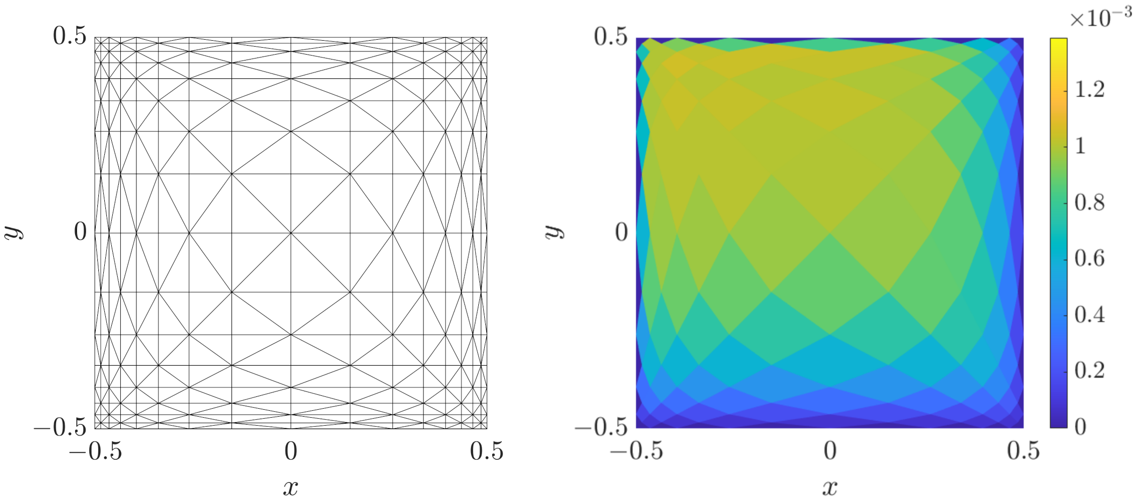
We derive an instance of the stochastic strong finite element problem by replacing $H_0^1(\Omega )$ in Problem 10 with a finite-dimensional subspace. In particular, we employ the space $X\subset H_0^1(\Omega )$ formed by continuous piecewise linear finite elements corresponding to a regular graded simplicial triangulation of $\Omega$, characterized by the number $M_{\mathrm{FE}}$ of finite element degrees of freedom. The triangulation of the computational domain $\Omega$ is shown in Figure 1. We estimate the spatial discretization error using simulations on a finer reference triangulation as a substitute for the exact solution.

3.2.2. Monte Carlo Method

We provide estimates of the expectation and variance by discretizing the respective stochastic integrals using Monte Carlo quadrature in the sense of Section 2.1.1. To this end, we generate random samples $y_{}^1,\cdots ,y_{}^{N_{{\xi }_{}}}\in {\Xi }_{}$ according to the distribution ${\mathbb{P}}_{{\xi }_{}}$ with a standard pseudorandom number generator. A reference simulation with a higher number of samples delivers an estimate of the sampling error. An exemplary solution of Problem 10 approximated by an MCFE method is shown in the right plot of Figure 1.

3.2.3. Stochastic Galerkin Method

Stochastic Galerkin methods estimate the expectation and variance by directly evaluating the respective stochastic integrals, given a stochastic Galerkin solution based on a finite-dimensional subspace of $L_{{\xi }_{}}^2\left({\Xi }_{}\right)$. In general, a stochastic Galerkin finite element method applied to a linear elliptic problem with a random elliptic coefficient leads to a large, block-structured system of linear algebraic equations. In our case, however, the underlying random variables $y_1,\cdots ,y_K$ are independent and enter the bilinear form linearly, see (27). Under these conditions, it is possible to find a double-orthogonal polynomial basis which decouples the blocks in the system matrix [39,40]. The resulting block-diagonal system of equations can be solved efficiently due to the relatively small bandwidth and the ability to treat the blocks in parallel. To define a suitable double-orthogonal basis, we start with K spaces of possibly different dimensions, spanned by univariate Legendre polynomials over the interval $[-\sqrt{3},\sqrt{3}]$. We normalize the polynomials regarding the underlying uniform distribution and rotate the bases such that they consist of double-orthogonal univariate polynomials, as described in [39]. Finally, a tensor product of these univariate double-orthogonal polynomial bases forms a basis of an $M_{\mathrm{SG}}$-dimensional subspace $S\subset L_{{\xi }_{}}^2\left({\Xi }_{}\right)$. In our experiments, we use the same polynomial degree d in all directions. We assess the error associated with the choice of d by comparing with a reference solution using a higher degree.

3.2.4. Reduced Basis

The considered reduced-order models rely on POD spaces generated from snapshots of the underlying discretized solution. We choose $N_{{\mu }_{}}^{\mathrm{train}}=64$ as the number of training samples in the deterministic parameter domain. Consequently, Section 2.3 specifies the creation of the reduced spaces.

3.3. Computational Costs

We analyze the computational costs associated with the MCRB and SGRB method. We focus on the offline costs, that is, the costs necessary to set up the reduced models and estimators. The costs of the online phase depend on the dimensions of the reduced spaces which are not known a priori. The computational costs of the online phase for the numerical examples considered in Section 3 are briefly analyzed in Section 4.

The offline phase consists of several steps which are necessary to construct the reduced-order models and estimators. In the following, we list the computations that dominate the overall costs. At first, all coercivity constants necessary for the estimators in Section 2.1.3 and Section 2.2.3 are computed. As a second step, we construct the reduced spaces for the primal and dual Problems 2, 4, 6 and 8 based on the POD Algorithm 1. This must be done five times for the MCRB method (one primal problem and four dual problems) and four times for the SGRB method (one primal problem and three dual problems). Constructing a reduced space consists of the snapshot computations and the singular value decomposition of the weighted snapshot matrix. The systems of equations to compute the snapshots for the SGRB method are decoupled with respect to the SG basis because of the double-orthogonal polynomials. An overview of the listed computations is given in

Table 3. Primary computational costs of the offline phase of the MCRB approach.

#	Dimension	Problem to Solve	Output
$N_{{\xi }_{}}$	$M_{\mathrm{FE}}\times M_{\mathrm{FE}}$	eigenvalue problem	coercivity constant
$5N_{{\xi }_{}}·N_{{\mu }_{}}^{\mathrm{train}}$	$M_{\mathrm{FE}}\times M_{\mathrm{FE}}$	system of equations	snapshots
5	$M_{\mathrm{FE}}\times N_{{\xi }_{}}·N_{{\mu }_{}}^{\mathrm{train}}$	singular value decomposition	reduced basis

for the MCRB method and in

Table 4. Primary computational costs of the offline phase of the SGRB approach.

#	Dimension	Problem to Solve	Output
1	$M_{\mathrm{FE}}{M}_{\mathrm{SG}}\times M_{\mathrm{FE}}{M}_{\mathrm{SG}}$	eigenvalue problem	coercivity constant
$4M_{\mathrm{SG}}·N_{{\mu }_{}}^{\mathrm{train}}$	$M_{\mathrm{FE}}\times M_{\mathrm{FE}}$	system of equations	snapshots
4	$M_{\mathrm{FE}}{M}_{\mathrm{SG}}\times N_{{\mu }_{}}^{\mathrm{train}}$	singular value decomposition	reduced basis

for the SGRB method. We only state the problems that must be solved and their dimensions as we use the same algorithms for both methods. For the MCRB approach, the coercivity constant is computed $N_{{\xi }_{}}$ times, that is, for every MC sample of the random parameters, see Section 2.1.3. Using a strictly positive lower bound instead reduces the costs to the computation of one single eigenvalue problem.

One can see that the difference in the offline costs primarily results from the difference between the number of MC samples $N_{{\xi }_{}}$ and the dimension of the SG basis $M_{\mathrm{SG}}$. Consequently, the SGRB method will be competitive in scenarios where $M_{\mathrm{SG}}$, that is, the number of random parameters and the polynomial degree, is small. For problems with a large number of random parameters, $M_{\mathrm{SG}}$ can become orders of magnitude larger than $N_{{\xi }_{}}$.

3.4. Numerical Results

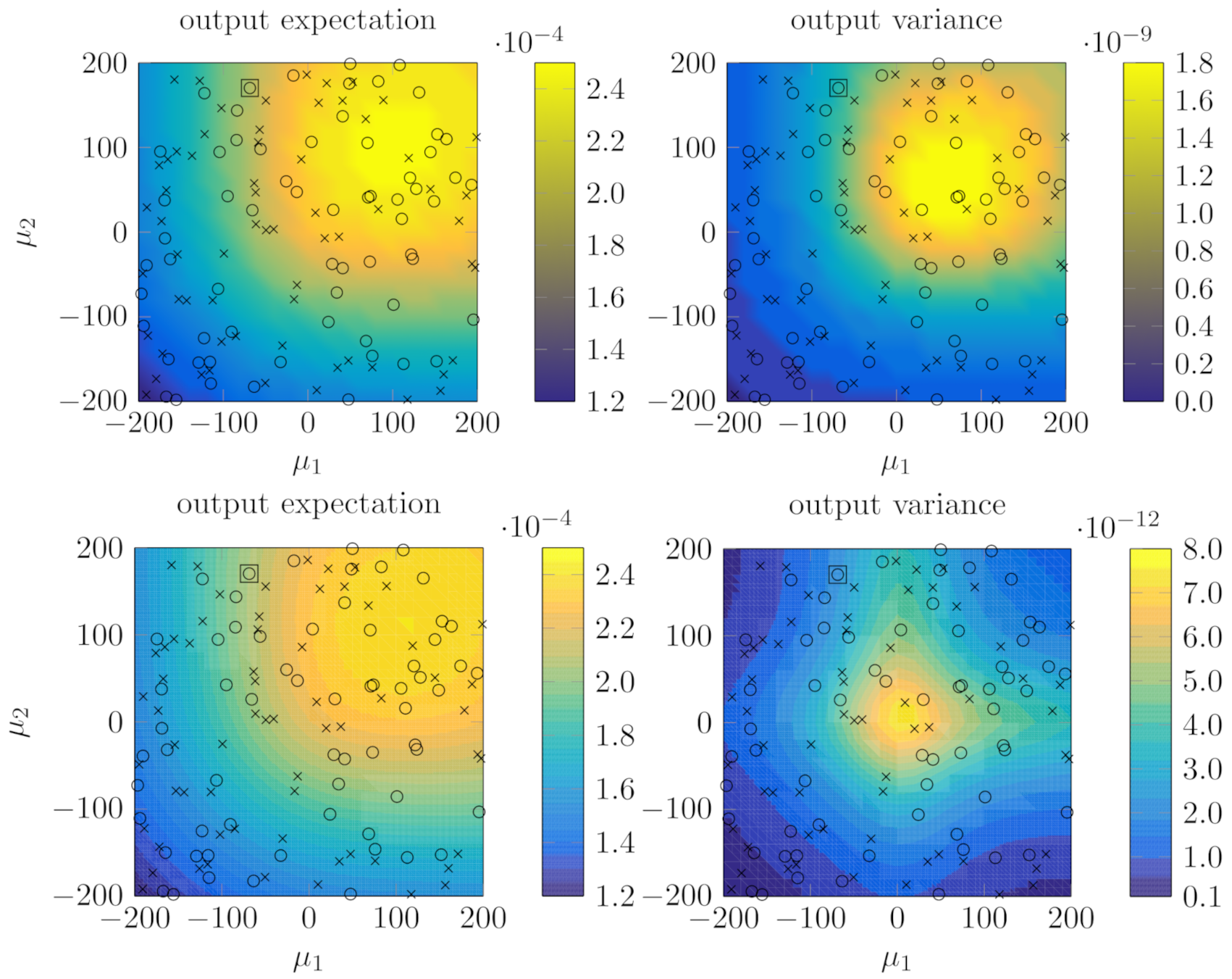
Figure 2 presents the parameter-dependent output statistics obtained with the default parameter-dependent SGFE models. The top row shows the results for test case 1 and the bottom row shows the results for test case 2. The crosses in Figure 2 correspond to the snapshot training parameter values provided by the pseudorandom number generator. Additionally, Figure 2 shows the test parameter values that are used to assess the model.

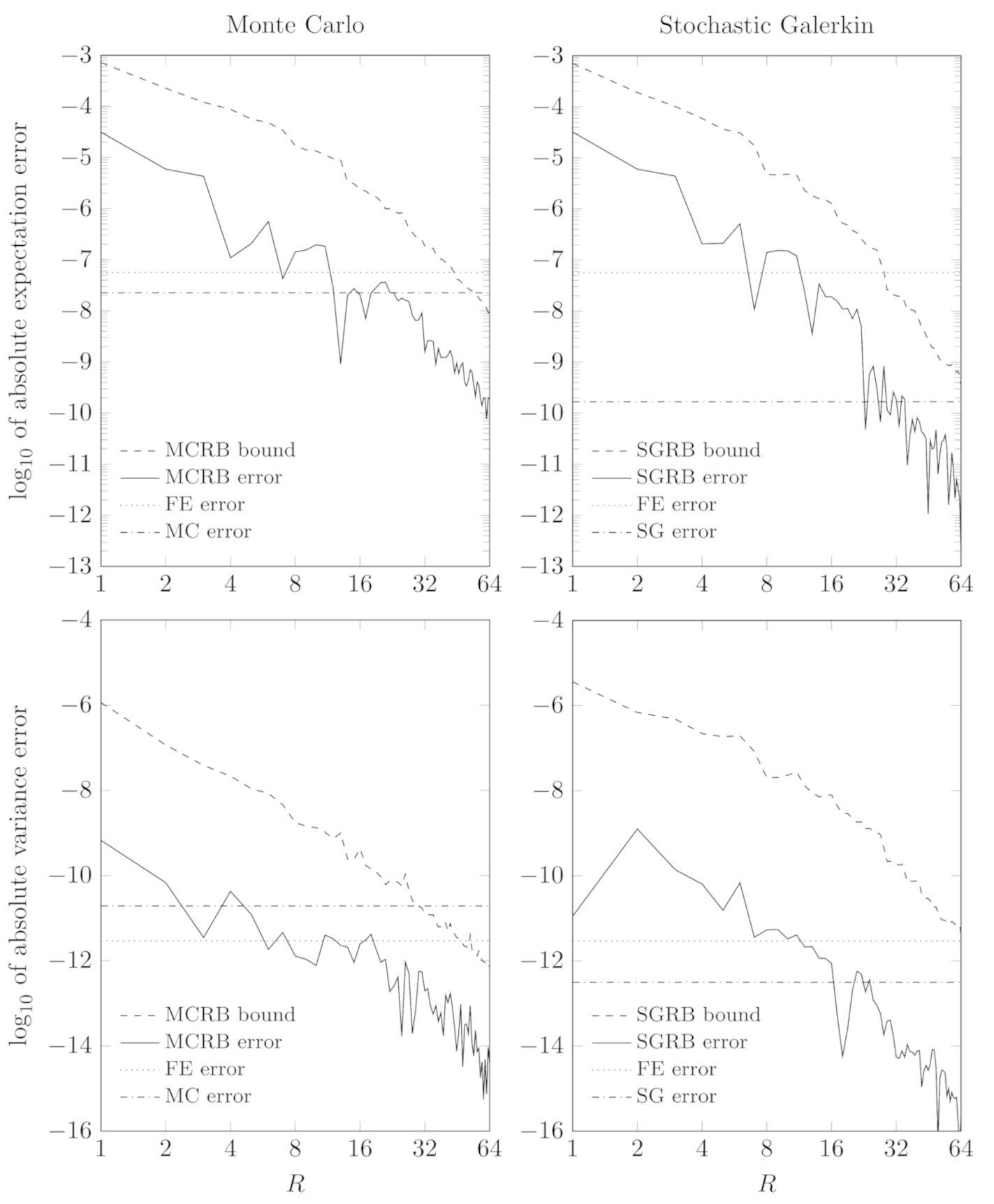
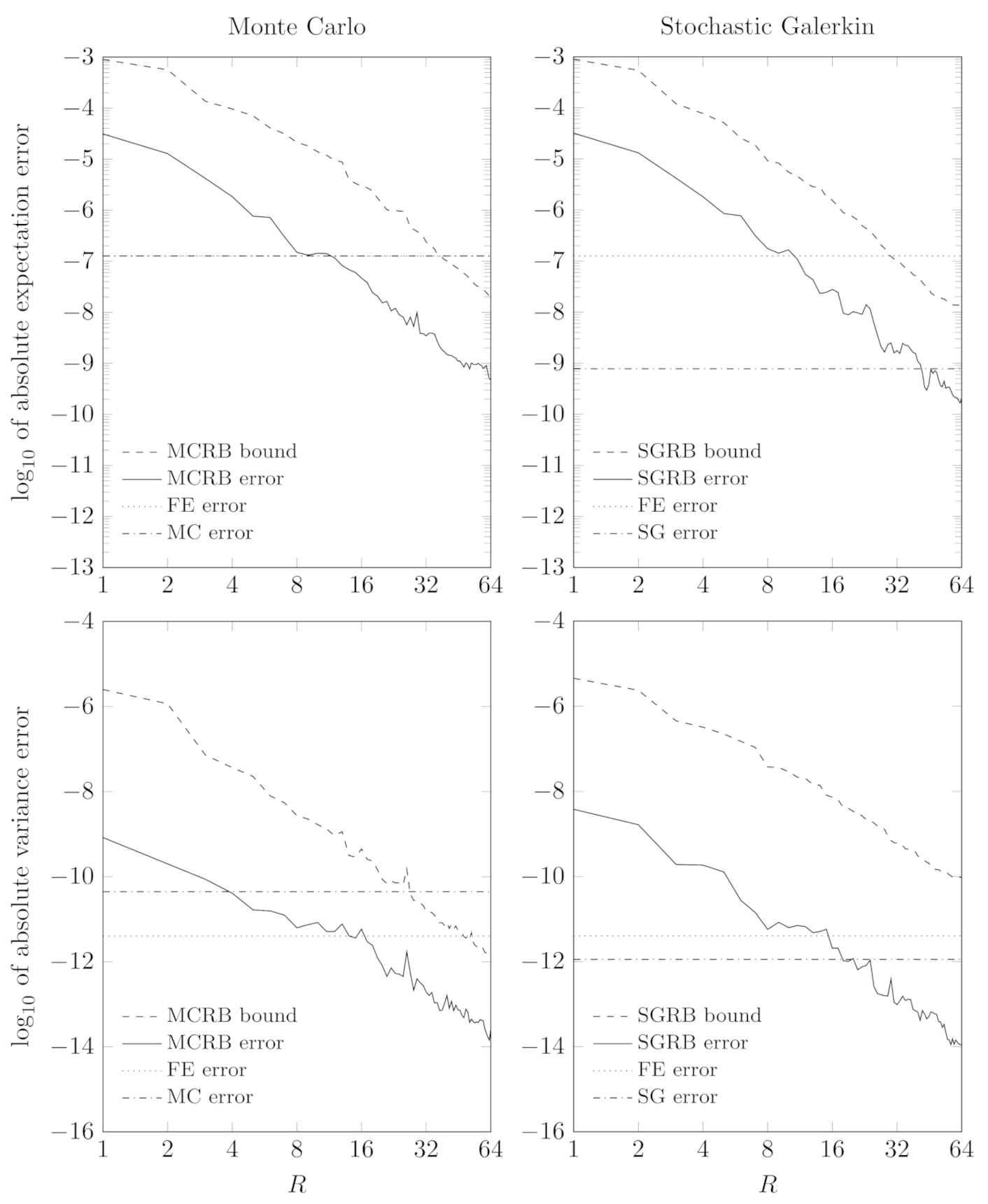
The reduced basis estimates of the output statistics together with the respective error bounds are provided by Theorems 3 and 4 for the MCRB method, and Theorems 6 and 7 for the SGRB method. First, we validate the error bounds for a single random realization of the deterministic parameter, marked by a square in Figure 2. The convergence regarding the number of reduced basis functions R is presented in Figure 3 and Figure 4. The error components of the underlying discretized solutions are provided as references. Looking at the discretization errors only, we see that the number of MC samples is sufficient to approximate the expectation, but is actually too small to balance the FE error in case of the variance. The SG error, on the other hand, is smaller than the FE error in all cases, which provides evidence that the stochastic Galerkin discretization of the stochastic domain is sufficiently fine. Concerning the reduced basis models, we observe that $R\approx 16$ reduced basis functions are sufficient to obtain reduced-order estimates which are on a par with the full-order estimates in all considered cases. The plots suggest that all error bounds converge at the same rates as the respective errors. This is useful, because it implies that efficiency of the error bounds does not become significantly worse when the number of reduced basis functions is increased.

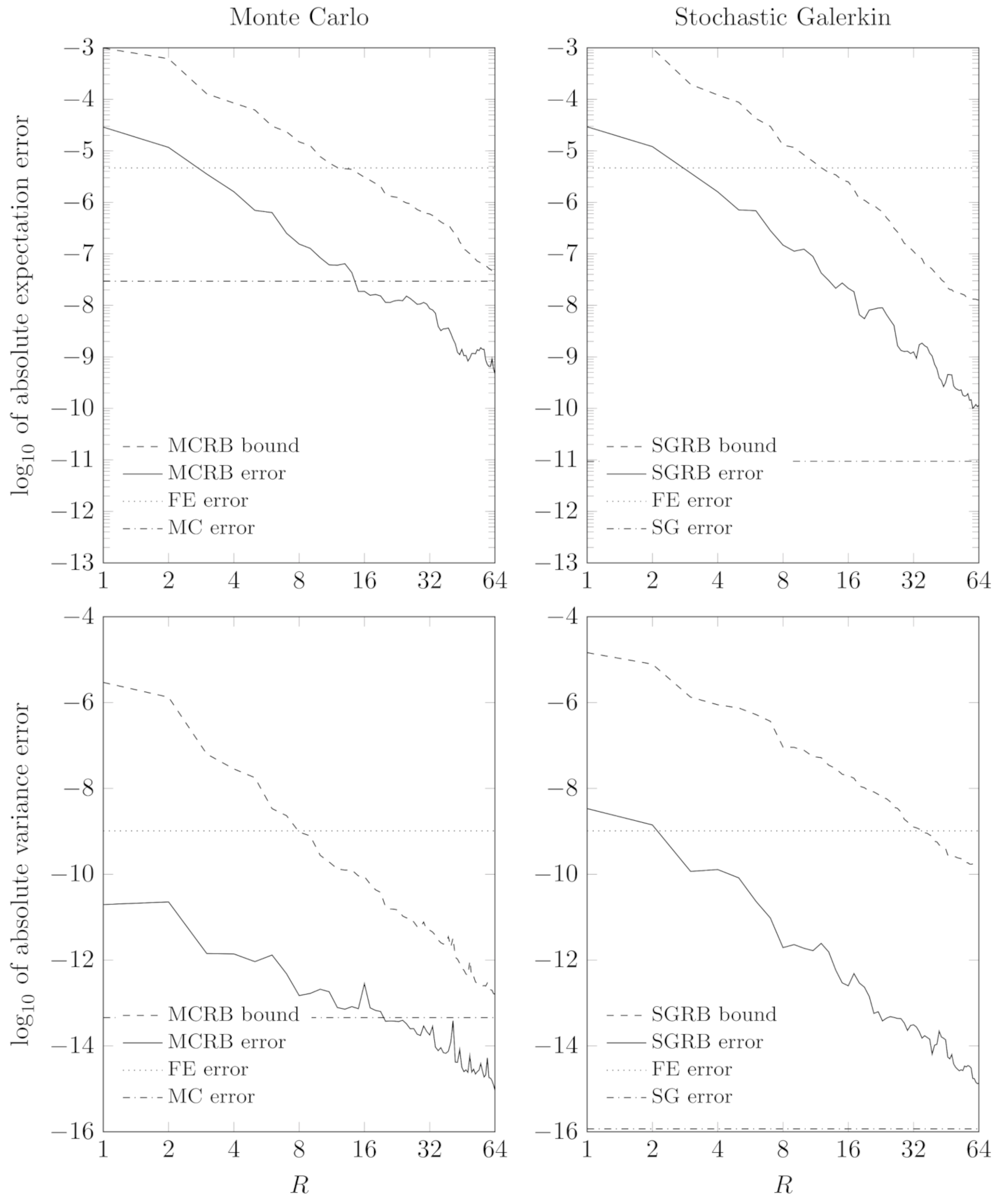
We assess the convergence globally over $\mathcal{P}$ in order to confirm that the point-wise observations in the deterministic parameter space provided by Figure 3 and Figure 4 is not a lucky coincidence. To this end, we employ an $L_{}^2\left(\mathcal{P}\right)$-norm, approximated using Monte Carlo quadrature with $N_{{\mu }_{}}^{\mathrm{test}}=64$ samples shown as circles in Figure 2. The convergence results are presented in Figure 5 and Figure 6. Since we have averaged over the parameter space, the plots appear less random than the plots in Figure 3 and Figure 4. The convergence of the estimates and the corresponding bounds correspond quite well. Moreover, the MCRB and SGRB methods perform similarly in terms of accuracy per number of basis functions.

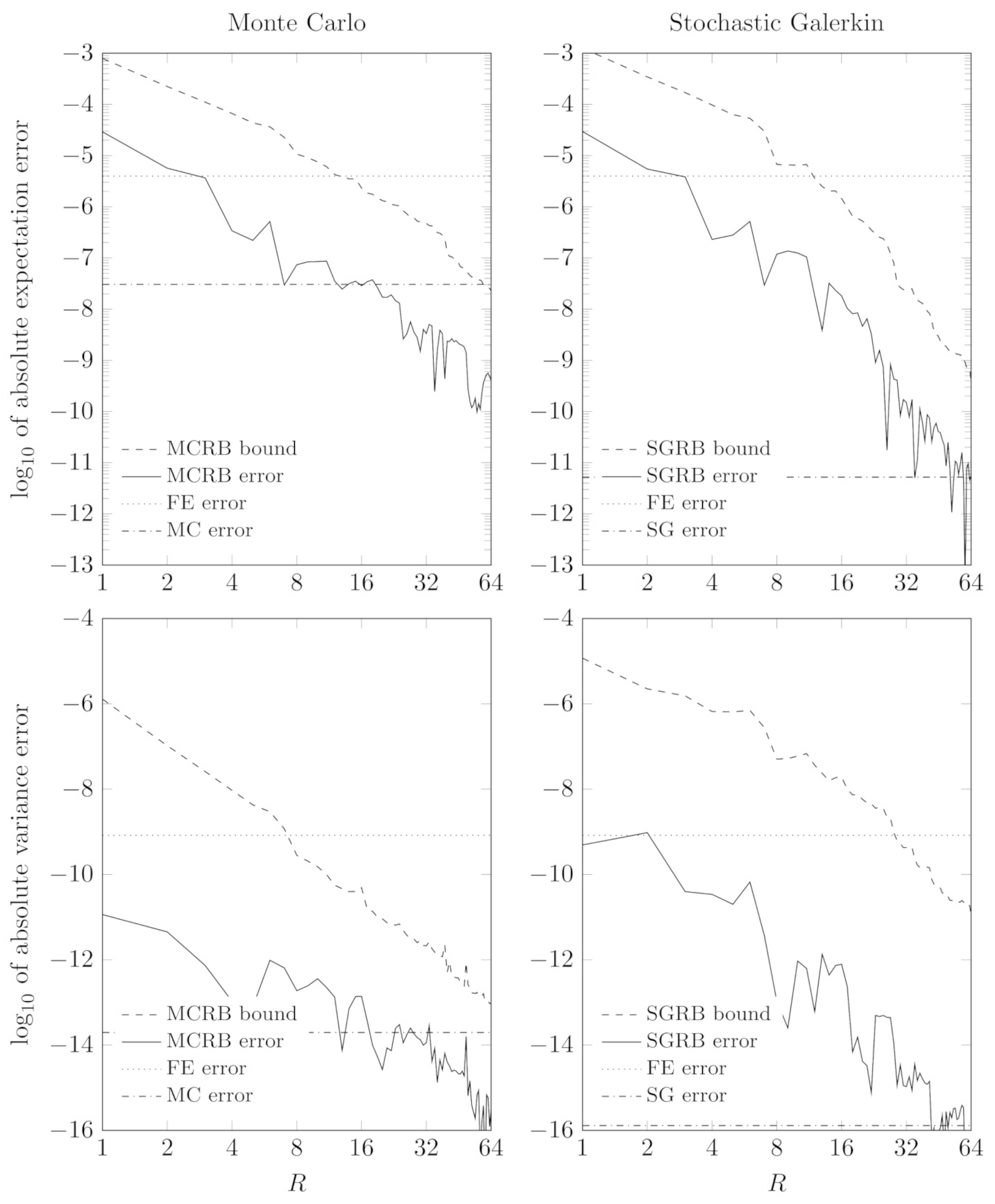
In Figure 3, Figure 4, Figure 5 and Figure 6, it appears that the SGRB error bound over-estimates the actual error more severely (by four orders of magnitude) than the MCRB error bound (two orders of magnitude). A closer inspection of the individual components of the error estimate reveals that for larger R, the lower-order term involving the continuity factor becomes responsible for the major portion of the error estimate. In particular, for $R=64$ at the parameter point corresponding to Figure 3, the terms on the right-hand side of Theorem 7 amount to approximately $4.2·{10}^{-12}$, $1.2·{10}^{-19}$ and $5.2·{10}^{-14}$, respectively.

4. Discussion

We have investigated the use of MCRB and SGRB methods to estimate parameter-dependent statistics of functional outputs of interest of elliptic PDEs with parametrized random and deterministic input data. Our analysis is restricted to linear elliptic variational problems and cannot be generalized to nonlinear or non-elliptic equations in a straightforward way. It further relies on the fact that all parameters enter the equations affinely. For more complex, non-affine input representations, additional approximation steps, such as empirical interpolation techniques, are necessary for the analysis and methods to be applicable. Furthermore, reduced-order methods, as considered in this work, are only reasonable surrogates for the high-fidelity models when the parameter-dependent output of interest lives on a low-dimensional manifold. This is the case for our numerical examples, as can be seen by the fast decay of the error contributions.

We have observed that the SGRB method can deliver estimates of the expectation and variance of linear outputs with an accuracy similar to the MCRB method for the convection–diffusion–reaction model problems. Additionally, the SGRB error bounds regarding the expected value were very close to the respective MCRB bounds in our experiments. Concerning the variance, the presented SGRB bounds overestimate the error more severely than the available MCRB bounds, which opens opportunities for future improvement of the SGRB variance bound. Nevertheless, the MCRB and SGRB variance bounds both converge at the same order depending on the number of reduced basis functions. This behavior is reflected by the theory, which predicts the same order of convergence in terms of dual norms of residuals.

The MCRB statistical output estimates and error bounds require a Monte Carlo sampling of the reduced quantities point-wise in the random parameter domain. In our convection-diffusion-rection model problems, 1024 samples were sufficient to balance the finite element error for the expectation, but an accurate prediction of the variance would require even more samples. The SGRB estimates and bounds, on the other hand, are obtained by an exact integration of the corresponding reduced basis expansions in the setup phase of the reduced-order model, and, thus, do not rely on Monte Carlo sampling. As a consequence, the primal and dual SGRB problems need to be solved only once for each new deterministic parameter. This benefit comes at the cost of a more expensive offline phase. In our tests, the SGRB and the MCRB methods achieved a similar reduction of degrees of freedom for a given error tolerance. As a consequence, the possible online speedup of SGRB methods compared to MCRB methods is in the order of magnitude of the number of Monte Carlo samples. This is particularly attractive in scenarios where evaluating the reduced-order model shall be as inexpensive as possible, while the offline costs are not a primary concern.

References

- Morton, K.W. Numerical Solution of Convection-Diffusion Problems; Chapman & Hall: London, UK, 1996. [Google Scholar]
- Hesthaven, J.; Rozza, G.; Stamm, B. Certified Reduced Basis Methods for Parametrized Partial Differential Equations; Springer: Cham, Switzerland, 2016. [Google Scholar]
- Prud’homme, C.; Rovas, D.V.; Veroy, K.; Machiels, L.; Maday, Y.; Patera, A.T.; Turinici, G. Reliable real-time solution of parametrized partial differential equations: Reduced-basis output bound methods. J. Fluid. Eng. Trans. ASME 2002, 124, 70–80. [Google Scholar] [CrossRef]
- Quarteroni, A.; Manzoni, A.; Negri, F. Reduced Basis Methods for Partial Differential Equations; Springer: Cham, Switzerland, 2016. [Google Scholar]
- Boyaval, S.; Bris, C.; Maday, Y.; Nguyen, N.; Patera, A. A reduced basis approach for variational problems with stochastic parameters: Application to heat conduction with variable Robin coefficient. Comput. Methods Appl. Mech. Eng. 2009, 198, 3187–3206. [Google Scholar] [CrossRef]
- Haasdonk, B.; Urban, K.; Wieland, B. Reduced basis methods for parametrized partial differential equations with stochastic influences using the Karhunen–Loève Expansion. SIAM/ASA J. Uncertain. Quantif. 2013, 1, 79–105. [Google Scholar] [CrossRef]
- Chen, P.; Quarteroni, A.; Rozza, G. A weighted reduced basis method for elliptic partial differential equations with random input data. SIAM J. Numer. Anal. 2013, 51, 3163–3185. [Google Scholar] [CrossRef] [Green Version]
- Vidal-Codina, F.; Nguyen, N.C.; Giles, M.B.; Peraire, J. An empirical interpolation and model-variance reduction method for computing statistical outputs of parametrized stochastic partial differential equations. SIAM/ASA J. Uncertain. Quantif. 2016, 4, 244–265. [Google Scholar] [CrossRef] [Green Version]
- Spannring, C.; Ullmann, S.; Lang, J. A weighted reduced basis method for parabolic PDEs with random data. In Recent Advances in Computational Engineering; Schäfer, M., Behr, M., Mehl, M., Wohlmuth, B., Eds.; Springer International Publishing: Cham, Switzerland, 2018; pp. 145–161. [Google Scholar] [CrossRef] [Green Version]
- Newsum, C.; Powell, C. Efficient reduced basis methods for saddle point problems with applications in groundwater flow. SIAM/ASA J. Uncertain. Quantif. 2017, 5, 1248–1278. [Google Scholar] [CrossRef] [Green Version]
- Boyaval, S. A fast Monte–Carlo method with a reduced basis of control variates applied to uncertainty propagation and Bayesian estimation. Comput. Methods Appl. Mech. Eng. 2012, 241-244, 190–205. [Google Scholar] [CrossRef] [Green Version]
- Chen, P.; Schwab, C. Sparse-grid, reduced-basis Bayesian inversion: Nonaffine-parametric nonlinear equations. J. Comp. Phys. 2016, 316, 470–503. [Google Scholar] [CrossRef]
- Manzoni, A.; Pagani, S.; Lassila, T. Accurate solution of Bayesian inverse uncertainty quantification problems combining reduced basis methods and reduction error models. SIAM/ASA J. Uncertain. Quantif. 2016, 4, 380–412. [Google Scholar] [CrossRef] [Green Version]
- Chen, P.; Quarteroni, A. Accurate and efficient evaluation of failure probability for partial different equations with random input data. Comput. Methods Appl. Mech. Eng. 2013, 267, 233–260. [Google Scholar] [CrossRef]
- Venturi, D.; Wan, X.; Karniadakis, G.E. Stochastic low-dimensional modelling of a random laminar wake past a circular cylinder. J. Fluid. Mech. 2008, 606, 339–367. [Google Scholar] [CrossRef] [Green Version]
- Freitas, F.; Pulch, R.; Rommes, J. Fast and accurate model reduction for spectral methods in uncertainty quantification. Int. J. Uncertain. Quantif. 2016, 6, 271–286. [Google Scholar] [CrossRef]
- Pulch, R.; ter Maten, E. Stochastic Galerkin methods and model order reduction for linear dynamical systems. Int. J. Uncertain. Quantif. 2015, 5, 255–273. [Google Scholar] [CrossRef]
- Glas, S.; Mayerhofer, A.; Urban, K. Two ways to treat time in reduced basis methods. In Model Reduction of Parametrized Systems; Modeling, Simulation and Applications; Benner, P., Ohlberger, M., Patera, A., Rozza, G., Urban, K., Eds.; Springer International Publishing: Cham, Switzerland, 2017; Volume 17, Chapter 1; pp. 1–16. [Google Scholar] [CrossRef]
- Urban, K.; Patera, A. A new error bound for reduced basis approximation of parabolic partial differential equations. CR Math. 2012, 350, 203–207. [Google Scholar] [CrossRef] [Green Version]
- Wieland, B. Reduced Basis Methods for Partial Differential Equations with Stochastic Influences. Ph.D. Thesis, Universität Ulm, Ulm, Germany, 2013. [Google Scholar] [CrossRef]
- Vidal-Codina, F.; Nguyen, N.; Giles, M.; Peraire, J. A model and variance reduction method for computing statistical outputs of stochastic elliptic partial differential equations. J. Comput. Phys. 2015, 297, 700–720. [Google Scholar] [CrossRef] [Green Version]
- Huynh, D.B.P.; Peraire, J.; Patera, A.T.; Liu, G.R. Real-time reliable prediction of linear-elastic mode-i stress intensity factors for failure analysis. In Proceedings of the Singapore MIT Alliance Conference, Singapore, 7 July 2006. [Google Scholar]
- Sen, S. Reduced Basis Approximation and a Posteriori Error Estimation for Non-Coercive Elliptic Problems: Application to Acoustics. Ph.D. Thesis, Massachusetts Institute of Technology, Cambridge, MA, USA, 2007. [Google Scholar]
- Jiang, J.; Chen, Y.; Narayan, A. A Goal-Oriented Reduced Basis Methods-Accelerated Generalized Polynomial Chaos Algorithm. SIAM/ASA J. Uncertain. Quantif. 2016, 4, 1398–1420. [Google Scholar] [CrossRef]
- Dexter, N.C.; Webster, C.G.; Zhang, G. Explicit cost bounds of stochastic Galerkin approximations for parameterized PDEs with random coefficients. Comput. Math. Appl. 2016, 71, 2231–2256. [Google Scholar] [CrossRef] [Green Version]
- Nouy, A. A generalized spectral decomposition technique to solve a class of linear stochastic partial differential equations. Comput. Methods Appl. Mech. Eng. 2007, 4521–4537. [Google Scholar] [CrossRef] [Green Version]
- Tamellini, L.; Maître, O.L.; Nouy, A. Model reduction based on proper generalized decomposition for the stochastic steady incompressible Navier-Stokes equations. SIAM J. Sci. Comput. 2014, 36, A1089–A1117. [Google Scholar] [CrossRef] [Green Version]
- Powell, C.E.; Silvester, D.; Simoncini, V. An efficient reduced basis solver for stochastic Galerkin matrix equations. SIAM J. Sci. Comput. 2017, A141–A163. [Google Scholar] [CrossRef] [Green Version]
- Lee, K.; Elman, H.C. A preconditioned low-rank projection method with a rank-reduction scheme for stochastic partial differential equations. SIAM J. Sci. Comput. 2017, 39, S828–S850. [Google Scholar] [CrossRef] [Green Version]
- Powell, C.E.; Elman, H.C. Block-diagonal preconditioning for spectral stochastic finite-element systems. IMA J. Numer. Anal. 2009, 29, 350–375. [Google Scholar] [CrossRef] [Green Version]
- Müller, C.; Ullmann, S.; Lang, J. A Bramble–Pasciak conjugate gradient method for discrete Stokes equations with random viscosity. SIAM/ASA J. Uncertain. Quantif. 2019, 7, 787–805. [Google Scholar] [CrossRef]
- Elman, H.C.; Liao, Q. Reduced basis collocation methods for partial differential equations with random coefficients. SIAM/ASA J. Uncertain. Quantif. 2013, 1, 192–217. [Google Scholar] [CrossRef] [Green Version]
- Powell, C.; Lord, G.; Shardlow, T. An Introduction to Computational Stochastic PDEs, 1st ed.; Cambridge University Press: Cambridge, UK, 2014. [Google Scholar]
- Ngoc Cuong, N.; Veroy, K.; Patera, A.T. Certified real-time solution of parametrized partial differential equations. In Handbook of Materials Modeling: Methods; Yip, S., Ed.; Springer: Dordrecht, The Netherlands, 2005; pp. 1529–1564. [Google Scholar] [CrossRef]
- Kunisch, K.; Volkwein, S. Control of the Burgers equation by a reduced-order approach using proper orthogonal decomposition. J. Optim. Theory App. 1999, 102, 345–371. [Google Scholar] [CrossRef]
- Ghanem, R.G.; Spanos, P.D. Stochastic Finite Elements: A Spectral Approach; Springer: New York, NY, USA, 1991. [Google Scholar]
- LeMaître, O.P.; Knio, O.M. Spectral Methods for Uncertainty Quantification—With Applications to Computational Fluid Dynamics; Springer: New York, NY, USA, 2010. [Google Scholar]
- Elman, H.; Silvester, D.; Wathen, A. Finite Elements and Fast Iterative Solvers—With Applications in Incompressible Fluid Dynamics, 2nd ed.; Oxford University Press: Oxford, UK, 2014. [Google Scholar]
- Babuška, I.; Tempone, R.; Zouraris, G.E. Galerkin finite element approximations of stochastic elliptic partial differential equations. SIAM J. Numer. Anal. 2004, 42, 800–825. [Google Scholar] [CrossRef]
- Frauenfelder, P.; Schwab, C.; Todor, R.A. Finite elements for elliptic problems with stochastic coefficients. Comput. Methods Appl. Mech. Eng. 2005, 194, 205–228. [Google Scholar] [CrossRef]
Figure 1.
Computational domain with triangulation (left) and exemplary mean value of the solution of Problem 9 with a randomly chosen convective velocity, approximated by an MCFE approach (right).
Figure 2.
Parameter-dependent output expectation and variance for the functional l given by (26). The top row shows the results for test case 1 and the bottom row shows the results for test case 2. Crosses mark the snapshot parameter values. The square marks the parameter value corresponding to Figure 3 and Figure 4. Circles mark the parameter values used to obtain Figure 5 and Figure 6.
Figure 3.
Log–log plots of the errors in the approximation of the expectation (top row) and variance (bottom row) of a linear functional with an MCRB method (left column) and an SGRB method (right column) depending on the dimension R of the reduced spaces, for a random point in the deterministic parameter domain, for the first test case. Respective error bounds and approximate FE/SG/MC discretization errors.
Figure 4.
Log–log plots of the errors in the approximation of the expectation (top row) and variance (bottom row) of a linear functional with an MCRB method (left column) and an SGRB method (right column) depending on the dimension R of the reduced spaces, for a random point in the deterministic parameter domain, for the second test case. Respective error bounds and approximate FE/SG/MC discretization errors.
Figure 5.
Log–log plots of the errors in the approximation of the expectation (top row) and variance (bottom row) of a linear functional with an MCRB method (left column) and an SGRB method (right column) depending on the dimension R of the reduced spaces, measured in terms of an approximate -norm, for the first test case. Respective error bounds and approximate FE/SG/MC discretization errors. It is a coincidence that the approximate FE and MC errors of the estimated expectation are very close in this outcome of the random experiment.
Figure 6.
Log–log plots of the errors in the approximation of the expectation (top row) and variance (bottom row) of a linear functional with an MCRB method (left column) and an SGRB method (right column) depending on the dimension R of the reduced spaces, measured in terms of an approximate -norm, for the second test case. Respective error bounds and approximate FE/SG/MC discretization errors.