
A Revisit of Implicit Monolithic Algorithms for Compressible Solids Immersed Inside a Compressible Liquid


McCoy School of Engineering, Midwestern State University, 3410 Taft Blvd., Wichita Falls, TX 76308, USA
Fluids 2021, 6(8), 273; https://0-doi-org.brum.beds.ac.uk/10.3390/fluids6080273
Submission received: 10 June 2021
/
Revised: 16 July 2021
/
Accepted: 22 July 2021
/
Published: 3 August 2021
(This article belongs to the Special Issue Fluid Structure Interaction: Methods and Applications)
Abstract
:With the development of mature Computational Fluid Dynamics (CFD) tools for fluids (air and liquid) and Finite Element Methods (FEM) for solids and structures, many approaches have been proposed to tackle the so-called Fluid–Structure Interaction or Fluid–Solid Interaction (FSI) problems. Traditional partitioned iterations are often used to link available FEM codes with CFD codes in the study of FSI systems. Although these procedures are convenient, fluid mesh adjustments according to the motion and finite deformation of immersed solids or structures can be challenging or even prohibitive. Moreover, complex dynamic behaviors of coupled FSI systems are often lost in these iterative processes. In this paper, the author would like to review the so-called monolithic approaches for the solution of coupled FSI systems as a whole in the context of the immersed boundary method. In particular, the focus is on the implicit monolithic algorithm for compressible solids immersed inside a compressible liquid. Notice here the main focus of this paper is on liquid or more precisely liquid phase of water as working fluid. Using the word liquid, the author would like to emphasize the consideration of the compressibility of the fluid and the assumption of constant density and temperature. It is a common practice to assume that the pressure variations are not strong enough to alter the liquid density in any significant fashion for acoustic fluid–solid interactions problems. Although the algorithm presented in this paper is not directly applicable to aerodynamics in which the density change is significant along with its relationship with the pressure and the temperature, the author did revisit his earlier work on merging immersed boundary method concepts with a fully-fledged compressible aerodynamic code based on high-order compact scheme and energy conservative form of governing equations. In the proposed algorithm, on top of a uniform background (ghost) mesh, a fully implicit immersed method is implemented with mixed finite element methods for compressible liquid as well as immersed compressible solids with a matrix-free Newton–Krylov iterative solution scheme. In this monolithic approach, with the simple modulo function, the immersed solid or structure points can be easily located and thus the displacement projections and force distributions stipulated in the immersed boundary method can be effectively and efficiently implemented. This feature coupled with the key concept of the immersed boundary method helps to avoid topologically challenging mesh adjustments and to incorporate parallel processing commands such as Message Passing Interface (MPI) and further vectorization of the numerical operation. Once these high-performance procedures are implemented coupled with the monolithic implicit matrix-free Newton–Krylov iterative scheme with immersed methods, effective and efficient reduced order modeling techniques can then be employed to explore phase and parametric spaces. The in-house developed programs are at the moment two-dimensional. Furthermore, based on the same approach implemented in one-dimensional test example with one continuum immersed in another continuum, such monolithic implicit matrix-free Newton–Krylov iterative approach can be extended for the study of composites with deformable aggregates and matrix.
1. Introduction
Fluid-Structure interactions (FSI) are ubiquitous in many engineering problems. Many research efforts have been invested in the development of modeling methods over the past few decades [1,2,3,4]. In practice, iterations are used between existing finite element methods (FEM) for solids and computational fluid dynamics (CFD) for fluids [5,6]. In engineering practices, such iterative approaches are effective and convenient, yet complex dynamic behaviors of coupled systems can also be filtered out [7,8]. Furthermore, mesh adaption processes such as the arbitrary Lagrangian Eulerian (ALE) and other mesh updating methods can be topologically challenging and computationally prohibitive [9,10,11,12,13]. In this paper, the focus is on the immersed boundary method and its concepts which are initially established in applied mathematics communities. Interface tracking procedures also include level set methods [14,15], immersed interface methods [16,17], and front tracking methods [18,19,20] which have been proposed to eliminate or bypass numerical problems associated with large motions of immersed objects [21,22,23,24,25]. Immersed methods do provide a very direct and simple coupling between immersed deformable solids with the surrounding fluid without specific interface tracking, which enable effective and efficient exploration of phase and parametric spaces in the design of complex FSI systems [26,27,28,29]. Since its inception [30,31,32], the immersed boundary method has been employed for the solutions of wave propagation in cochlea [33], swimming motions of marine worms [34], wood pulp fiber dynamics [35], and biofilm processes [36]. In fact, it has been discovered that the modeling philosophy of immersed methods is similar to the fictitious domain method [28,37,38,39]. In fact, such a principle can also be implemented to handle deformable solids immersed in another deformable solid medium as discussed in Ref. [40]. In early developments of immersed boundary methods, immersed elastic fibers are employed to construct various objects. As proposed in Ref. [41], torsion, bending, and transverse shear effects have also been added to immersed structures, namely beams instead of fibers. In this paper, the author would like to revisit immersed methods for compressible FSI systems ranging from acoustic fluid-solid interactions to compressible (or rather nearly incompressible) liquid interacting with deformable structures. In particular, mixed finite element formulations are used for both immersed solids and background fluids [42,43]. The communication between immersed solids and background fluids is accomplished with various kernels or radial-based interpolation functions widely implemented for meshless methods [44]. Such delta functions provide a higher order smoothness and can be extended to non-uniform fluid grids [45,46,47]. The focus of this paper is on some earlier results presented by the author and his collaborators [41,43,48,49], in particular those of acoustic fluid-solid interaction systems for which mixed finite element formulations and mixed finite elements which either satisfy the Inf-Sup conditions or pass the numerical Inf-Sup tests are essential in lieu of immersed methods. Similar immersed methods have already been implemented to electrokinetics and mass and heat transfers [48,50,51]. A fairly comprehensive review from the perspective of a merger between traditional aerodynamics and the immersed boundary method is available in Ref. [52].
2. Formulations and Theories
2.1. Mixed Finite Element Formulations
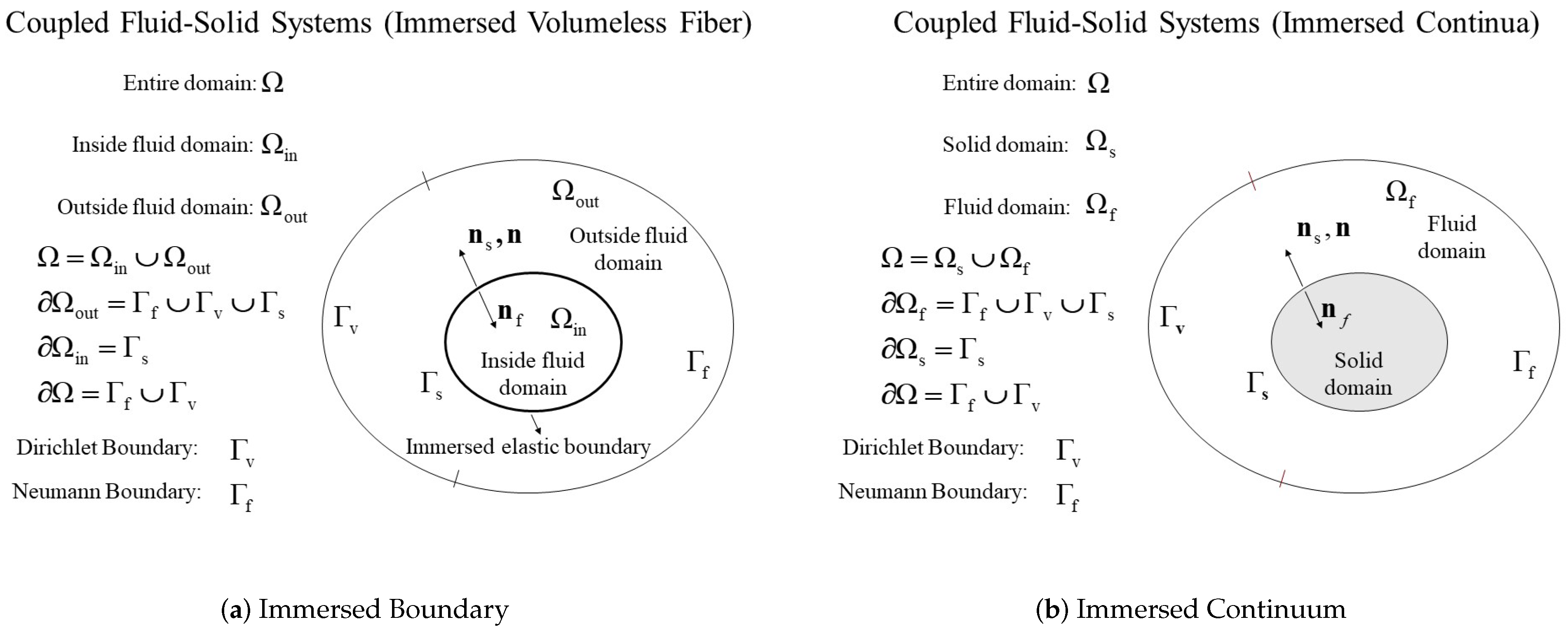
The key feature of immersed methods is to allow independent Lagrangian mesh of immersed solids to move on top of the background fluid which consists of a fixed Eulerian mesh. However, in order to be consistent with the actual physics, it is important to combine the immersed domain () and the physical exterior domain () into a complete background domain () as illustrated in Figure 1 and Figure 2. It is this complete domain that stays the same for any instantaneous position of the immersed continuum. Thus, there will be no need for frequent mesh adjustments. In fact, a background uniform mesh, namely ghost mesh is often used to effectively locate the vicinity of the immersed solids with modulo functions.
As illustrated in Refs. [53,54], the underlining principle of immersed methods is the energy conservation. In summary, the energy and power inputs to the fluid domain introduced by the immersed solids or immersed structures are identical to those from the equivalent body forces. To secure this key feature, the same delta function or kernel function must be used in both the distribution of the resultant nodal forces and the interpolation of the solid velocities based on the surrounding or rather background fluid velocities. In fact, this treatment in immersed methods can be viewed as the synchronization of the fluid motion with the solid motion within the immersed solid domain , namely . This important feature is also very similar to what is employed in the fictitious domain methods [37,38] along with the so-called distributed Lagrange multipliers as the equivalent body forces. Although in theory, the equivalent body forces can be directly calculated along with independent fluid and solid velocity vectors [55], the coupling of equivalent body forces and solid motions is implicit and nonlinear. Therefore, a matrix-free Newton–Krylov iterative procedures must be established to link both fluid and solid domains. Moreover, if the surrounding fluid is viscous and incompressible, the immersed solid or immersed structure must be incompressible in immersed methods and vice versa [56,57,58,59].
In this work, we review the implemented mixed finite element formulations for both compressible immersed solids or rather nearly incompressible solids and compressible liquid or rather nearly incompressible fluid. First, the weak form of the fluid-solid system can be written as
with
In continuum model for Newtonian fluids, the stress components is a combination of the pressure p and the deviatoric stress components ,
with .
Furthermore, the continuity equation of the compressible viscous fluid can be expressed as
where is the bulk modulus of the fluid.
Notice here we focus on liquid or more precise liquid phase of water as working fluid in the context of acoustic fluid-solid interactions namely the pressure variations are not strong enough to alter the water density in any significant fashion as in the case of underwater detonation where strong shock will trigger both phase transition of water and density changes must be included. Moreover, from
we have
For water, the bulk modulus is around and the density is around . It is clear that as long as the pressure variation is within the ambient pressure which is . The change of the water density is very minimum and should be ignored, so is the density of the immersed solid. Notice that when we deal with the air as the working fluid, fully-fledged energy conservation form of governing equations must be used along with non-oscillatory time incremental schemes [60,61].
Likewise, for immersed solids, the solid stress components can be decomposed as the pressure and the deviatoric stress components ,
In nonlinear mechanics, the solid deformation gradient is introduced along with the Green-Lagrangian strain component , also defined in the tensor form as with an identity matrix . Consequently, the energy conjugate stress of the Green-Lagrangian strain, namely the second Piola–Kirchhoff stress can be derived from the elastic energy , which is often related to the three invariants of the Cauchy-Green deformation tensor also defined in the tensor form as .
We must also point out that the solid domain and the material point position all refer to the current solid configurations, and for clarity they could be denoted as and , respectively. To properly introduce the material constitutive laws, we must first introduce elastic energy , which is often related to the invariants of the Cauchy-Green deformation tensor . A typical hyperelastic material can be described by the Mooney-Rivlin material model with large displacements and large strains. Hence, the strain energy potential at time t, is defined as
where the invariants are functions of the invariants , namely , , and with , , and .
In the formulations for acoustoelastic FSI systems, in order to avoid locking issues due to high bulk modulus for almost compressible solids, an additional elastic energy term , or is added to the elastic energy , along with solid unknown pressure . In the mixed finite element formulation, is an independent pressure unknown completely different from the background fluid pressure p,
where is the solid bulk modulus and stands for the determinant of the deformation gradient.
To delineate this pressure unknown from the pressure calculated based on the volumetric strain and the bulk modulus, we introduce
Naturally, the continuity equation becomes a constraint between the pressure unknown expressed as and the pressure as the function of the volumetric strain expressed as . In the displacement-based finite element formulation, such a constraint is strictly enforced, with . However, for almost incompressible materials with large bulk modulus, which covers many soft materials such as biological materials, the displacement-based finite element formulation will introduce so-called checkerboard pressure distributions and need to be replaced with mixed finite element formulations or combined with reduced integration techniques. Therefore, the second Piola-Kirchhoff stress can be expressed as
with .
Of course, to relate to the expression in Equation (7), the solid Cauchy stress can often be recovered from the second Piola-Kirchhoff stress, which is an energy conservative dual of the Green-Lagrangian strain,
In immersed methods, within the immersed domain, the solid displacement is dependent on the velocity of the fluid occupying the same immersed domain. Hence, the primary unknowns for the coupled fluid-solid system are the fluid velocity , the fluid pressure p, and the solid pressure . Define the Sobolev spaces, the weak form of governing equations can be expressed as: , , , which includes , and find and , , such that
For the fluid domain the following interpolations are introduced for the entire domain :
where and are the interpolation functions at node I for the fluid velocity vector and the fluid pressure; and , , , and represent the nodal values of the discretized fluid velocity vector, admissible fluid velocity variation, fluid pressure, and admissible fluid pressure variation, respectively.
Please note that the interpolation functions for the velocity vector unknowns in general are denoted by the superscript v, the independent pressure unknowns for immersed solids are denoted by and the independent pressure unknowns for background fluids are denoted by p.
Likewise for the solid domain , the discretization is based on the following:
where and are the interpolation functions at node J for the solid displacement vector dependent of the background fluid velocity vector and the independent solid pressure unknowns; and , , , and stand for the nodal values of the discretized solid displacement vector, admissible solid displacement variation, solid pressure, admissible solid pressure variation, respectively.
Now if we substitute both discretizations (13) and (14) into Equation (12), we can have the following discretization of the weak form: , , , which includes ,
Therefore, in the entire domain , the arbitrariness of the fluid velocity variations , fluid pressure variations , and independent solid pressure variations yields four equations for three velocity components and one pressure at each fluid node denoted as I and one equation for the independent solid pressure at each solid node denoted as J,
where the residuals are defined as
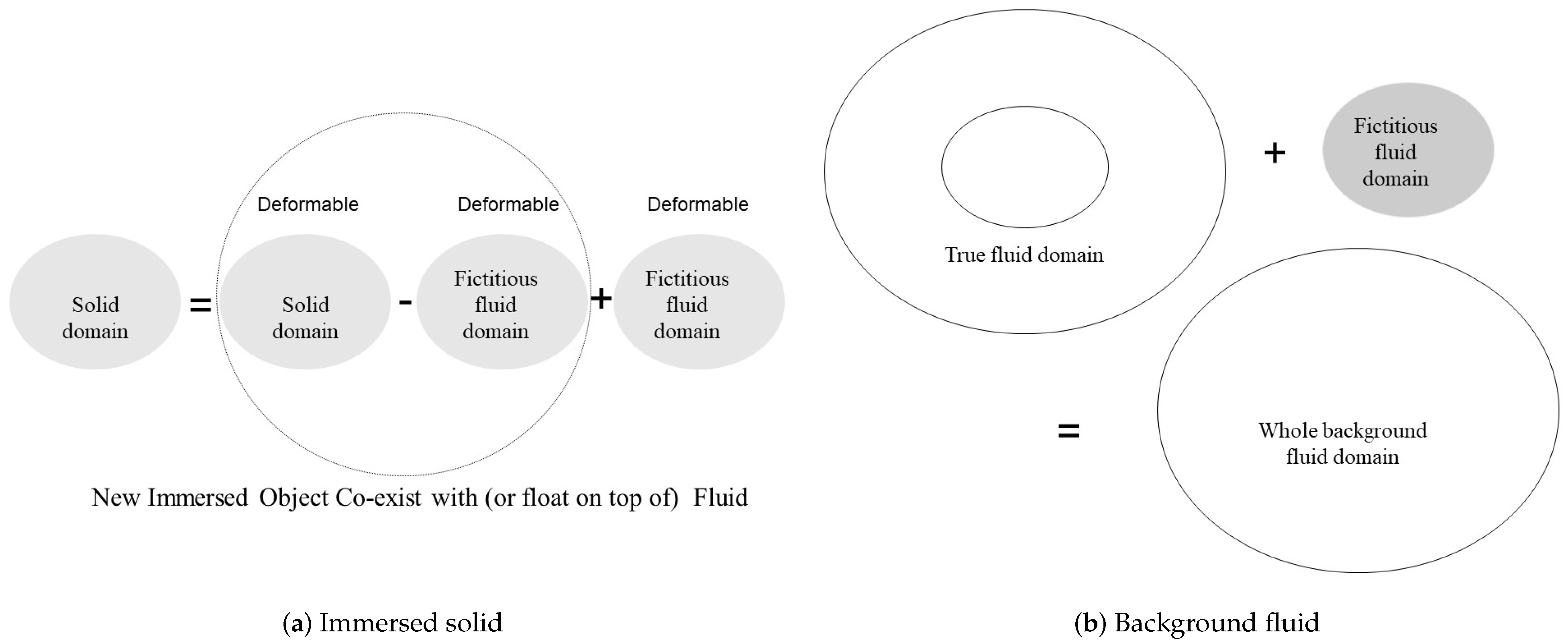
Please note that in both Equations (15) and (17) an implicit function is introduced to map from to , namely from the fluid mesh to the solid mesh, with the kernel functions. It is the implicit and nonlinear mapping between the immersed solid and the background fluid that consolidates the solid displacement unknowns with the fluid velocity unknowns. This nonlinear mapping can be better illustrated in specific nestings of subroutines although it is difficult to assign explicit analytical expression. Furthermore, a mapping function represents the mapping from the fluid domain implemented with background ghost mesh to the immersed sold domain the position of which is identified by the modulo function and projection will make that mapping efficient and straightforward. Furthermore, both Equations (12) and (15) are fully-fledged nonlinear form of the governing equation before any linearization. In fact, in the monolithic approach, the linearization will be coupled with the geometrical increment of the immersed solids in the program. The geometrical nonlinearity of the moving structures/solids are hidden in the so-called solid domain which is also occupied by the fluid. Therefore, the immersed solid in computation is the original solid subtract the background fluid which is physically not present as depicted in Figure 1 and in our monolithic implementation will also be constrained to follow the same kinematic motions as the immersed solid though with distinct fluid material constitutive laws identical to the surrounding fluid.
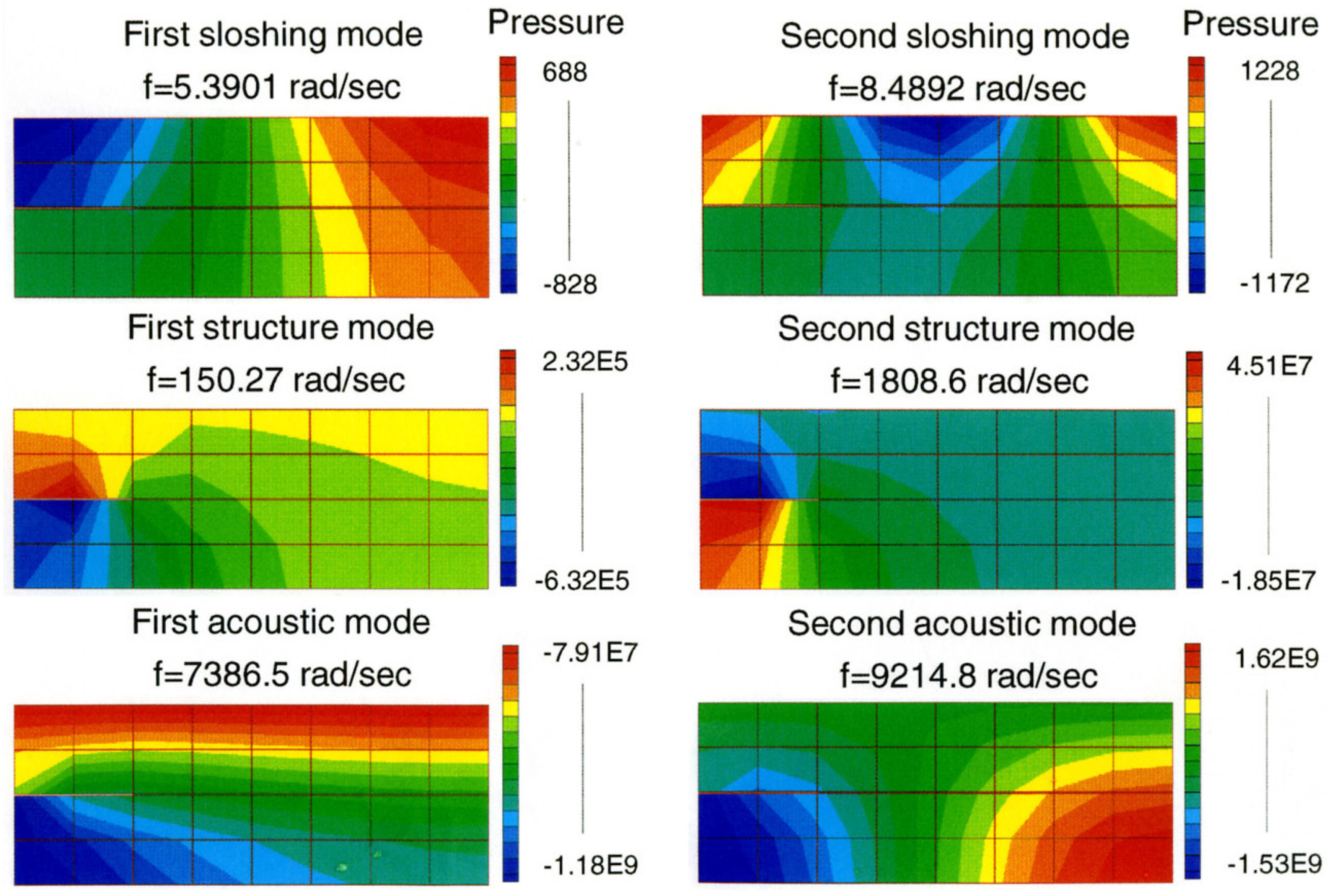
The isentropic compressible fluid formulation adopted in this paper with a constant density is in fact the same mixed finite element formulations developed for acoustoelastic FSI systems [62,63]. With sufficient mesh resolution and time step, pressure wave propagation and related scattering and radiation phenomena can be modeled. In general, small strain and small deformation assumptions are introduced for the acoustoelastic FSI systems. Therefore, immersed methods which have the advantage of automatically tracking the FSI interfaces is not necessary for this type of linear FSI systems [53,54]. However, with immersed solids, in nonlinear acoustic FSI model with finite interfacial motions, the monolithic implicit Newton-Krylov iterative procedure with immersed methods becomes essential. Furthermore, in the acoustoelastic FSI with free surface as illustrated in Figure 3, we have also demonstrated that with the same mixed finite element formulation for both acoustic fluid and immersed two-dimensional solid mimicking the immersed flexible structure, free surface modes No. 1 and 2 representing low frequency sloshing modes, solid modes No. 3 and 4 with intermediate frequency coupled or wet structural modes, along with clearly high and low pressure on top and bottom of the immersed structure, and acoustoelastic modes No. 5 and 6 with constant pressure on free surface can be evaluated in one monolithic coupled system eigenvalue problem. Moreover, with numerically stable mixed finite element formulation and mixed elements satisfying the Inf-Sup conditions, even a very coarse mesh can yield insightful results for fully coupled FSI systems. Naturally, the mesh density must be significantly higher if our aim in the simulation is to capture the high frequency range such as the acoustoelastic FSI models instead of the lower frequency ranges such as the wet structural modes or slowing modes as illustrated in Figure 3. The simple fact that a fairly coarse mesh as depicted in Figure 3 could capture coupled frequencies and corresponding modes from low to high ranges demonstrates the promise of this monolithic coupled code with mixed finite element formulations for immersed compressible solids and compressible (or rather nearly incompressible) liquid with constant density.
2.2. Stability Analysis
For nonlinear FSI analysis discussed in this paper, the incremental iteration within each time step involves a linearized transient analysis, hence, after transformation, the following equation is considered:
where is an effective load vector, and represent the effective stiffness matrix block corresponding to displacement unknowns and pressure unknowns, respectively [4].
The stability of such mixed finite element formulations with corresponding mixed elements is based on ellipticity and Inf-Sup conditions, which are necessary and sufficient conditions for well-posedness.
(a) Ellipticity Condition:
where , and .
(b) Inf-Sup Condition:
where the constant is independent of the mesh size h and the bulk modulus.
The Inf-Sup condition as depicted in (20) for mixed finite element formulations is elegant and useful, although the analytical proof for specific mixed elements and systems can be very difficult [64]. In practice, numerical Inf-Sup tests as discussed in [4,65] with eigenvalues or singular values associated with the coupling matrix are often employed.
2.3. Kernel Functions
The discretized delta functions implemented in the original Immersed Finite Element Methods proposed in Refs. [39,58,59] are the same as those in the so-called reproducing kernel particle methods (RKPM) or meshless finite element methods [44,66,67,68,69]. In immersed methods, as pointed out in Refs. [53,54], to ensure the energy conservation, we must employ the same discretized delta function for the distribution of solid nodal forces and the interpolation from the background fluid velocities to the immersed solid velocities. Moreover, the modified window function can also be used in the discretized delta function for non-uniform meshing for the background fluid domain. Both wavelet and smooth particle hydrodynamics (SPH) methods belong to the same class of reproducing kernel methods where the "reproduced" function is derived as
with a projection operator or a window function .
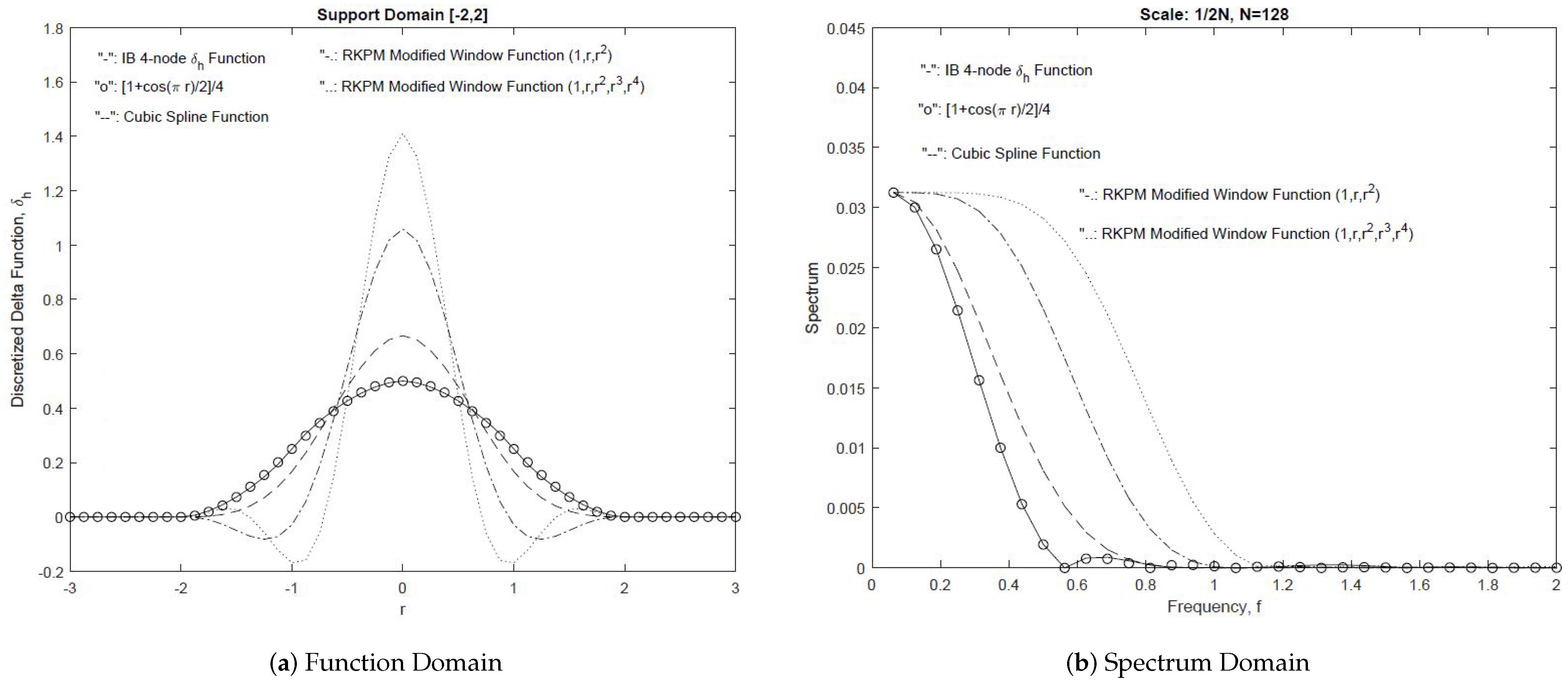
In essence, the window function is required to be flatter at in the Fourier domain as the order of reproducing gets higher. In Figure 4, we provide a comparison of various kernel functions in function and spectrum domains. With the increase of the reproducing order, for the same finite support region, the kernel functions approach to the ideal low pass filter.
As presented in detail in Ref. [58], consider first a one-dimensional case, in accordance with the translation invariance [31], for all r, where r is the parameter representing the position of the submerged boundary point and is scaled with respect to the grid size h, the discretized delta function satisfies , where C is a numerical constant. In addition, to uniquely define the discretized delta function for all r, we also have , where the selection of the moment depends on the number of support points. For instance, the discretized delta function with four support points is uniquely defined by the following:
- is a continuous function, with for ;
- For all r, ;
- For all r, ; and
- For all r, , where C is a numerical constant.
In general, for , the discretized delta function covers four non-zero support points. However, for the degenerate case of the 4-point discretized delta function centered at , we have five support points, namely . From the degenerate case, we can easily derive the constant C. Hence, we obtain the following four admissible branches of solutions for ,
Naturally, in the three-dimensional case, one of the smoothed approximations to the delta function is given by
It is interesting to point out that the discretized delta function in Equation (22) is very close to , with . Moreover, it is easy to confirm that the discretized delta function , with , defined in Equation (22), has continuity [70].
It is noted that in the current version of the implicit code the background ghost mesh is uniform which enables a very speedy estimate of the immersed solid location, and the order of accuracy is no more than two. Further work on the improvement of accuracy with adaptive meshing and much sharper FSI interface capturing techniques is discussed in Ref. [71].
3. Compressible Fluid Model for General Grids
In this section, unlike the early presentation of compressible fluid with working fluid as liquid, more specifically liquid form of water, in which the density is kept as constant due to the nearly compressible condition or rather large bulk modulus in the range of . In this section, we revisit some early attempt to expand the immersed boundary method to truly compressible fluid with working fluid as compressible air. Naturally, it is a common practice to adopt the conservative forms of governing equations for background compressible fluid domain. Notice that we adopt the same thermodynamic concepts with an increment of the specific enthalpy as where is the specific heat for constant pressure and T is the temperature in absolute scale, namely Rankine or Kelvin along with an increment of the specific internal energy as where is the specific heat for constant volume. Define the total specific mechanical energy as e, we have . Notice for ideal gas, we have with and the gas constant R is defined as where is the universal gas constant and M is the molar mass of the gas. Hence, the pressure p can also be written as with . Define the reciprocal of the density as the specific volume v, the first law of thermodynamics yields
where is the specific heat transferred to the system from the environment.
For isentropic (quasistatic, adiabatic, and reversible) gas, with , we have
Thus, combine with the ideal gas law, , we have
Consequently, for isentropic gas, the pressure p is governed by , where C is a constant. Furthermore, the speed of sound c is defined as or . Finally, use total specific enthalpy form, , and the Fourier law for thermal conduction, the conservation of energy can be written as
where stands for the rate of heat transfer from the surrounding environment to the system or control volume per unit volume, a so-called heat source.
4. Matrix-Free Newton–Krylov Iteration
4.1. Matrix Operation Specifics
To depict clearly the monolithic implicit immersed method with Newton–Krylov iterations, we start with the basic linear algebra concepts for the solution of general linear system of equations and the solution of eigenvalue problems. Assume is a matrix with m rows and n columns
the multiplication represents the linear combination of n columns of the matrix using n entities of the vector with and ; namely
where represents the ith column of the matrix .
Denote as a matrix with m rows and n columns
the multiplication represents the linear combination of m rows of the matrix using m entities of the vector with and ; namely,
where represents the jth row of the matrix .
Consequently, reduced row echelon form (rref) of the matrix after the left multiplication of the elementary matrix , namely the row combination and manipulation operation. Assume the rank of the matrix is r, the number of pivot variables is r, the number of free variables is , we derive
In general, if we have , the identity matrix corresponding to the pivot variables has the size , the free variable matrix has the size , the zero matrix has the size , and the zero matrix has the size . Introduce the new identity matrix with the size , the null space vectors can be expressed as
where the last rows of the transformation matrix , often called elementary matrix, are the left null vectors.
If , we have the full column rank, zero matrices and do not exist, namely there is no left null vector, and has the size , or , whereas if , we have the full row rank and the zero matrix has the size , or , namely there is no null vector.
4.2. Matrix-Free Newton–Krylov Iteration
In the matrix-free Newton–Krylov iteration, the target is the solution vector , or rather for fluid velocity unknowns, for fluid pressure unknowns, and for independent solid pressure unknowns. In this monolithic implicit immersed method with iterative solutions based on Newton–Krylov and generalized minimal residual method (GMRES) along with the numerical construction of the Jacobian matrix in the Newton-Raphson iteration, no specific analytical equation can be established other than an abstract operator which is implemented in recursive, iterative, and nested subroutines, the details of which are also presented and elaborated in the research manuscript by the author and his collaborator Professor Lucy Zhang in the Department of Mechanical Engineering of Rensselaer Polytechnic Institute [72]. We start our matrix-free Newton–Krylov with
with
A set of orthonormal vectors , with in the Krylov space and an upper-Hessenberg matrix . If we define and ,
and the remaining process in the GMRES method is to solve the least square problem:
Assuming is the length of the initial residual vector and is the unit vector, the first column of identity matrix,
, , preconditioning matrix , for , using the modified Gram-Schmidt orthogonalization process; we then have and , and for , we have and is updated with . Consequently, we obtain and . with
After we establish the elements of an upper Hessenberg matrix as well as an upper Hessenberg matrix , for , and , a factorization of is carried out
where the entities of the rotation processes are calculated as
Through this rotation process, the upper Hessenberg matrix is converted to a diagonal matrix with the coefficients defined as: for
Finally, the termination criteria: if , the solution vector , or rather , , , , , and is expressed as
or
Notice here for time increments, we use the trapezoidal temporal discretization is as the following,
and consequently,
and more importantly,
where can stand for the fluid interior nodal unknowns , the fluid-solid interface displacement unknowns , the solid interior nodal unknowns , the fluid interior pressure unknowns , the FSI coupled interface pressure unknowns , and the solid interior pressure unknowns .
Furthermore, the solid velocities are based on the projections of the background fluid velocities within the finite support region. Thus, the solid displacements at the FSI interface and the interior are integrated with the time integration scheme as stipulated in Equations (36) and (38). To be more specific, the update processes occur in very incremental iteration within one time step, which means, the positions of the immersed structures/solids are updated in all iteration within the matrix-free Newton–Krylov iteration.
For specific elaboration of the combination of Newton-Raphson iteration with Newton–Krylov iteration, we introduce
therefore, for
with , , , . Naturally, if or rather is sufficiently small, the second equation will be approximately satisfied, and the iteration will stop at the level when .
Moreover, for
with , , ; , , ; , , . Naturally, if or rather is sufficiently small, the third equation will be approximately satisfied, and the iteration will stop at the level when .
Finally, for
with , , , ; , , , ; , , , ; , , , . Naturally, if or rather is sufficiently small, the third equation will be approximately satisfied, and the iteration will stop at the level when .
5. Results and Verifications
In this section, we present several numerical examples to illustrate the efficacy and accuracy of the monolithic implicit immersed method with matrix-free Newton–Krylov iterations. The software developed through this work could be available upon request.
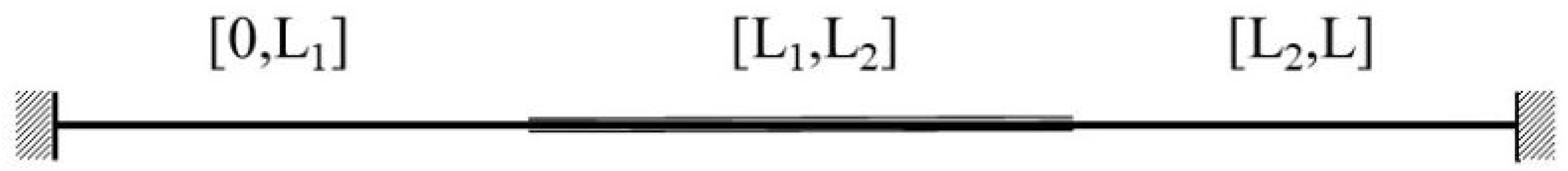
A model problem is introduced with a one-dimensional continuum within immersed in another one-dimensional continuum within as shown in Figure 5. The physical materials occupying region for one continuum and region for another continuum have a constant cross-section area A and are subjected to the gravitational acceleration g in x direction. Thus, the governing equations can be written as
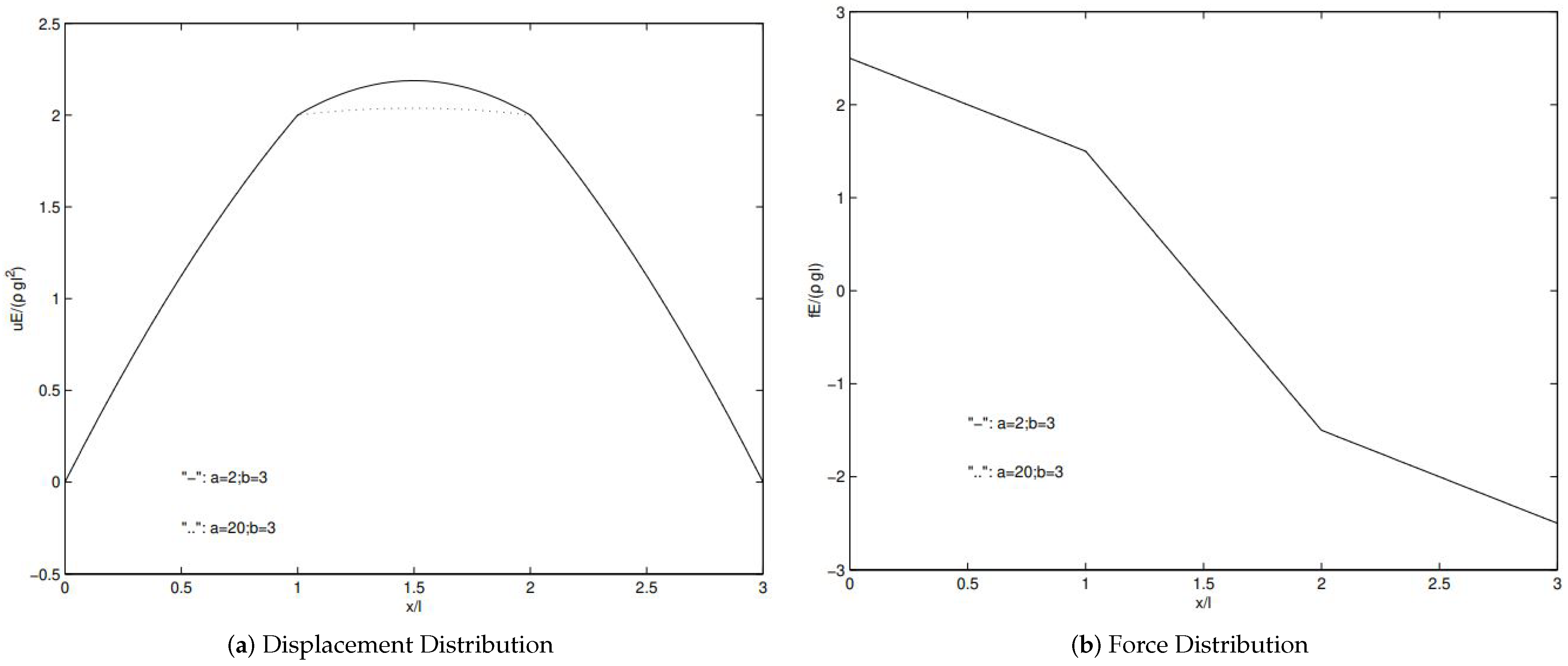
Equation (39) represent a set of two second-order partial differential equations (PDE) for both continuum with three connected regions, namely , , and . If we consider the boundaries marked by and dependent of time t and the displacement u, this problem will be non-trivial. For extreme conditions, let’s look at the corresponding static sets of equations, namely the right hand sides of Equation (39) which represent a set of two second-order ordinary differential equations (ODE). Finally, six constants will be introduced for all three regions, namely , , and , and the solution can be simply expressed as
Therefore, six constants will be derived based on the following six boundary conditions
In this model study, for simplicity, we assign , , , and . Moreover, we scale the three constants , with the same parameter . Finally, with , the solution of the six unknown constants can be determined from the boundary conditions (41) as
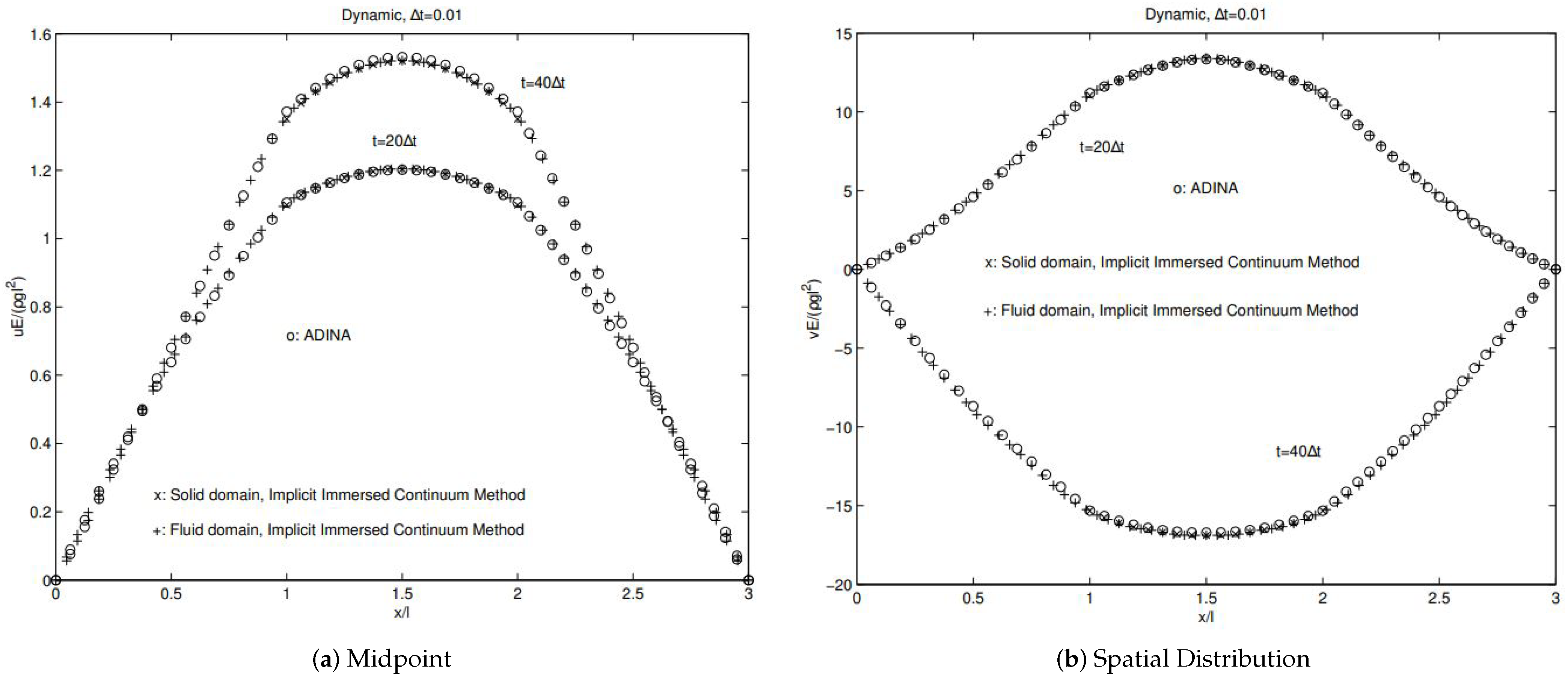
The comparisons with analytical solutions as well as existing computational fluid and solid software package such as ADINA as illustrated in Figure 6 and Figure 7 confirm the validity of the monolithic implicit immersed method with matrix-free Newton–Krylov iterations [39]. In addition, this simple one-dimensional model problem also confirms the subtle shift in math and engineering fields in which the background compressible fluids are often replaced with the background compressible solids [55].
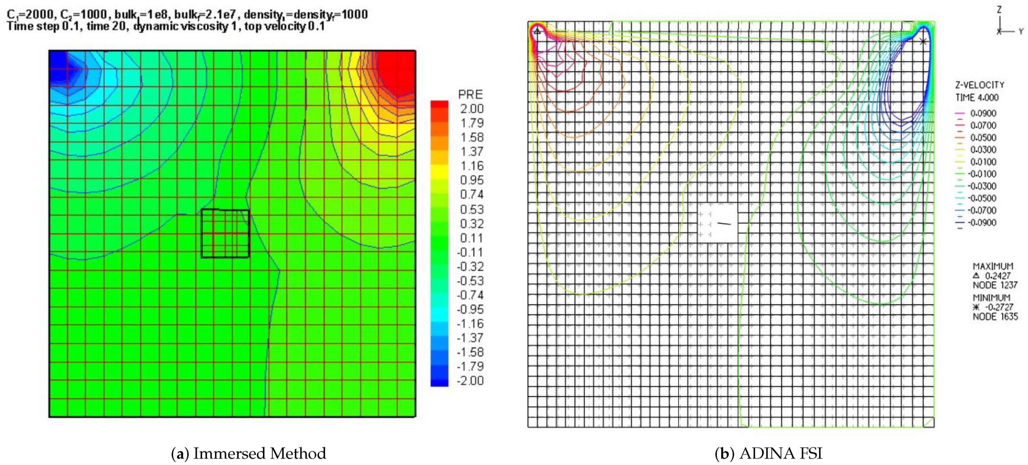
A clear validation and verification example is the driven cavity for viscous fluid with a dimension of m as illustrated in Ref. [39]. To compare the dynamical behaviors, the top shear velocity of the cavity is set as . The deformable solid is situated initially in the center of the cavity with zero velocity. To avoid the overlap of the mesh for the immersed solid and the background fluid mesh, we choose the typical immersed solid with the dimension of m. The submerged solid is made of a compressible rubber material with the material constant = and the density . For hard solids we use and . The case with hard solids resembles the same driven cavity problem with immersed rigid bodies [73]. In addition, the viscous fluid is represented with compressible model with a constant wave speed. Notice that in this acoustoelastic FSI example, the Mach number is much smaller than just as the case presented in Ref. [74]. Moreover, we have the dynamic viscosity , the bulk modulus , and the density .
It is evident that even with the coarse mesh used, the developed formulation with high-order elements provides reasonable results comparable to a reference solution. In addition, no spatial oscillation and checkerboard pressure bands are observed, as demonstrated in Figure 8. Of course, the proposed description can be further improved with refined meshes. As one of the main messages, we must point out that in engineering practice, before a large number of finite elements are used, it is always beneficial to employ coarse meshes with high-order elements to obtain a reasonable estimation of complicated problems.
In the implementation, the background fluid mesh is constructed for the entire cavity, which includes the space occupied by the immersed solids, consists of mixed finite elements as illustrated in detail in Refs. [4,64]. A typical immersed solid is represented by mixed finite elements. In the post computation presentation, we split each 9-node element into four 4-node elements. As a result, the velocity mesh will be two times denser than the pressure mesh. As shown in Figure 8, the mesh construction clearly demonstrates the philosophical difference between the monolithic implicit immersed method with matrix-free Newton–Krylov iterations and the traditional ALE approaches. In our method, the solid mesh is floating right on top of the background fluid mesh, whereas in the ALE formulation, the solid mesh is surrounded by the fluid mesh with a different mesh density.
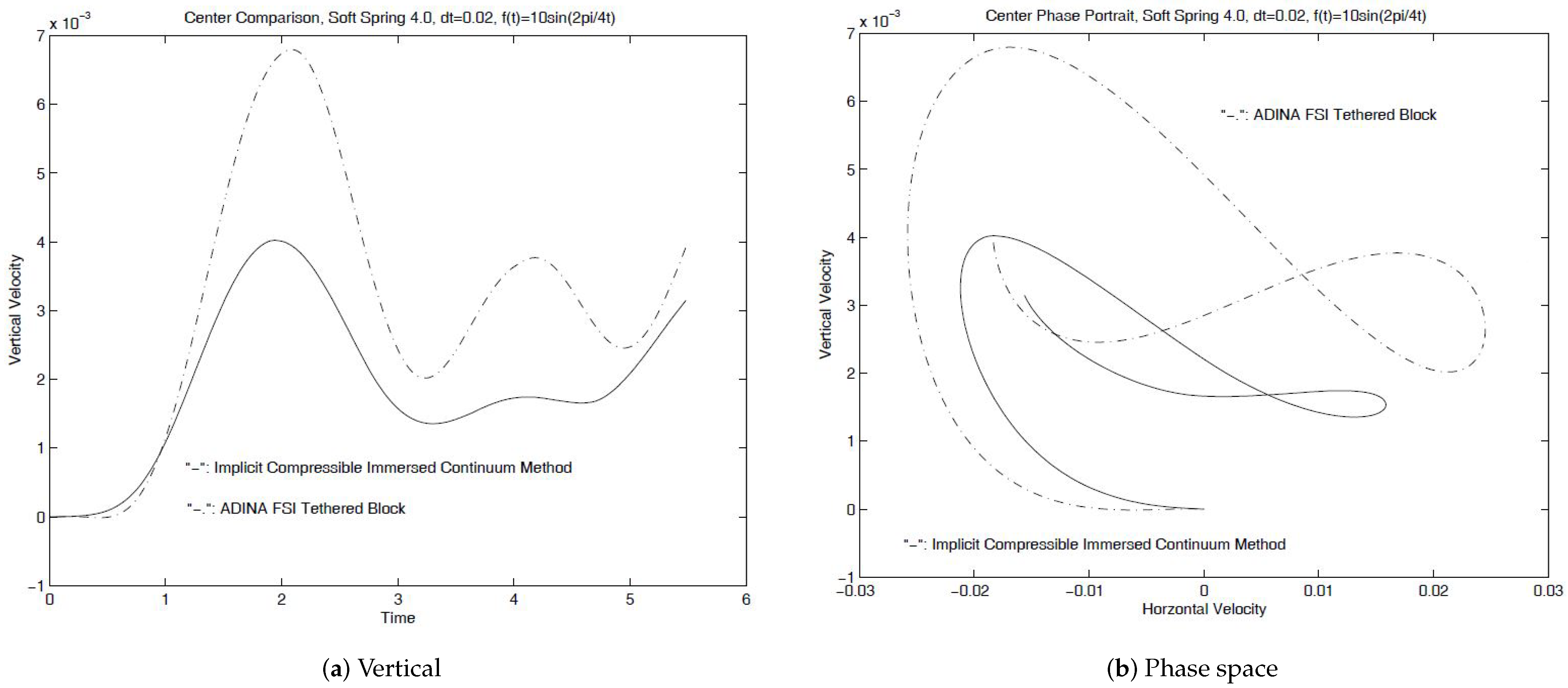
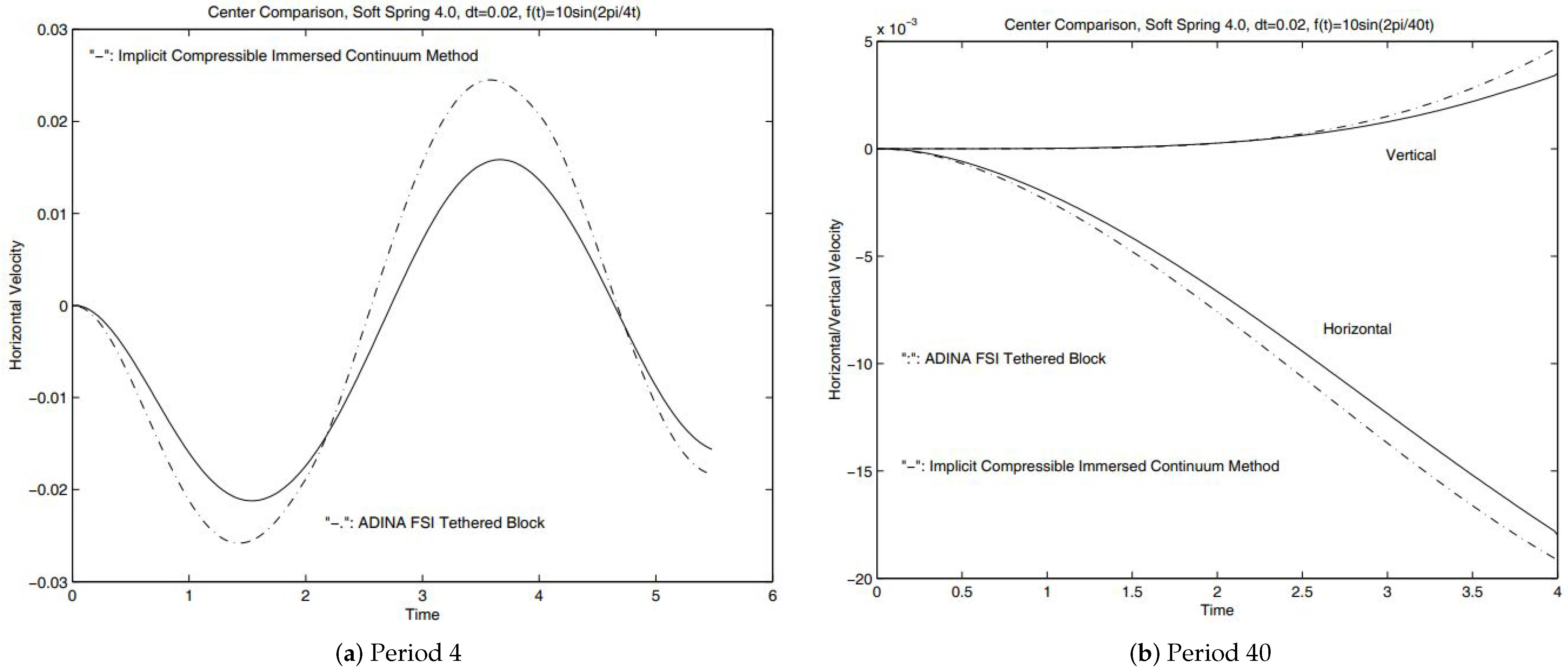
For the case with one immersed square solid, as long as the immersed solid does not move and deform significantly, it is still possible to solve this fluid-solid system with traditional modeling techniques such as the arbitrary Lagrangian-Eulerian (ALE) formulation. For the comparison of fixed immersed solid, we compare the velocity components of the midpoint of the immersed solid. With the same time step size, as shown in Figure 9, even with the coarse mesh of high-order mixed elements, the results from the monolithic implicit immersed method with matrix-free Newton–Krylov iterations and the ADINA FSI solver are very close. Considering the fact that these results are derived from two completely different approaches with entirely different meshes, these comparisons are very assuring. Moreover, for the case with the center of the immersed solid tethered with a soft spring (), despite the difference of the fluid mesh shown in Figure 8, the trajectories of the block center derived from the immersed continuum method and the ADINA FSI solver do match well with each other as depicted in Figure 9 and Figure 10. Further studies with different periods also demonstrate in Figure 10 that a slightly larger numerical viscous exists in comparison with the traditional computational approaches.
It is very important to point that the discretized delta function provides the possibility of linking the immersed solid node with the surrounding fluid nodes as done in meshless finite element methods. However, as pointed out in Ref. [56], the immersed solid node can also be restricted to communicate with the very finite element for the background fluid domain. As long as the virtual power input to the surrounding fluid is preserved, the concept of immersed methods will stay the same. This procedure is the same as the standard finite element procedure to distribute concentrated forces and to interpolate displacement/velocity within the element. Whether or not this procedure is as efficient as the meshless type of communication depends very much on the search algorithm for the purpose of locating the immersed solid nodes.
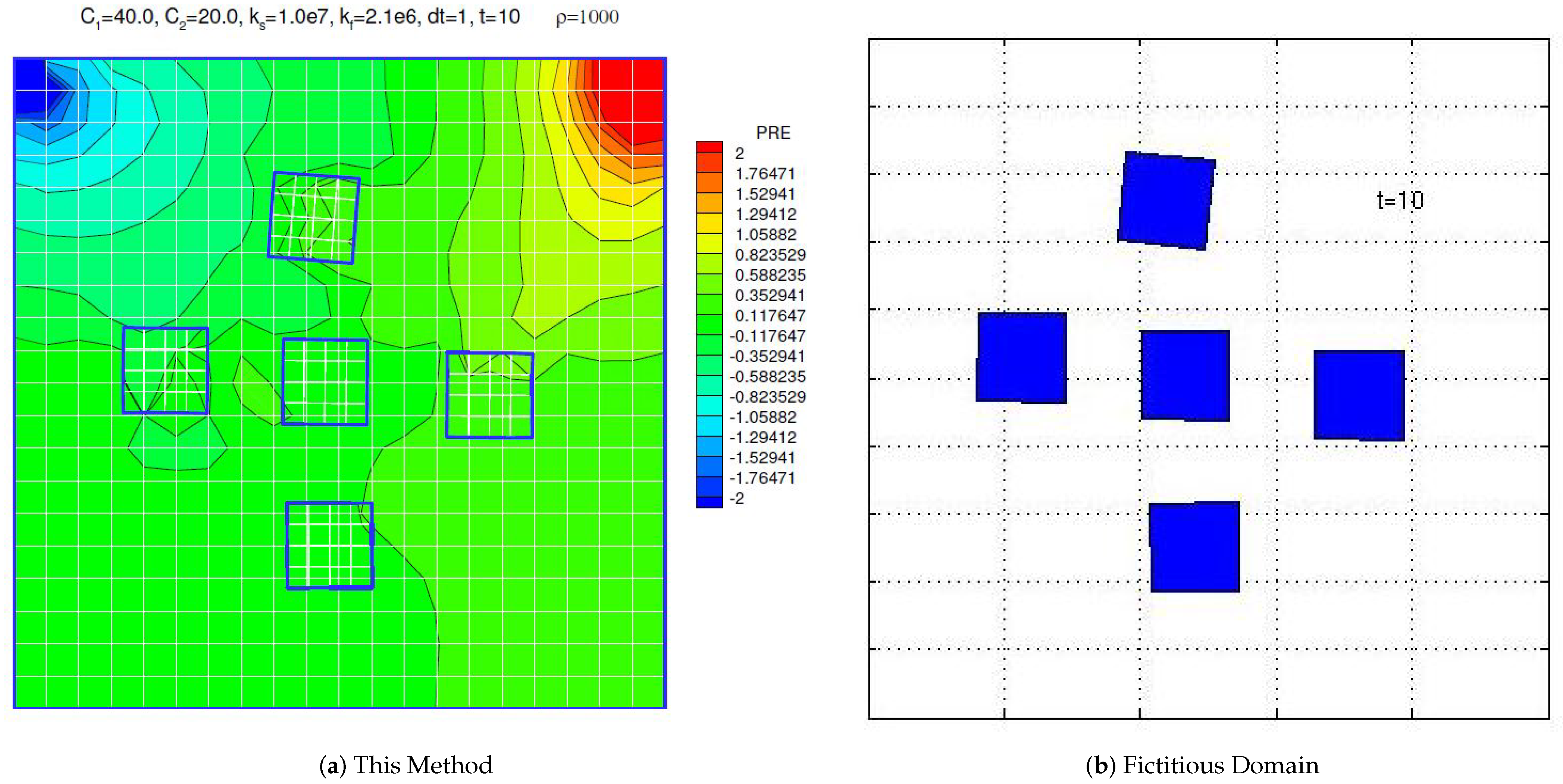
The benefit of the immersed methods is clear for the case with five immersed solids as illustrated in Figure 11. For this case, also depicted in Ref. [39], it is no longer feasible to use the ALE formulation, whereas it is relatively straightforward to add a few more deformable solids in the monolithic implicit immersed method with matrix-free Newton–Krylov iterations. The only possible comparison came from Professor Tsorng-Whay Pan in the Department of Mathematics of the University of Houston. The simulation animation can be accessed in Ref. [73].
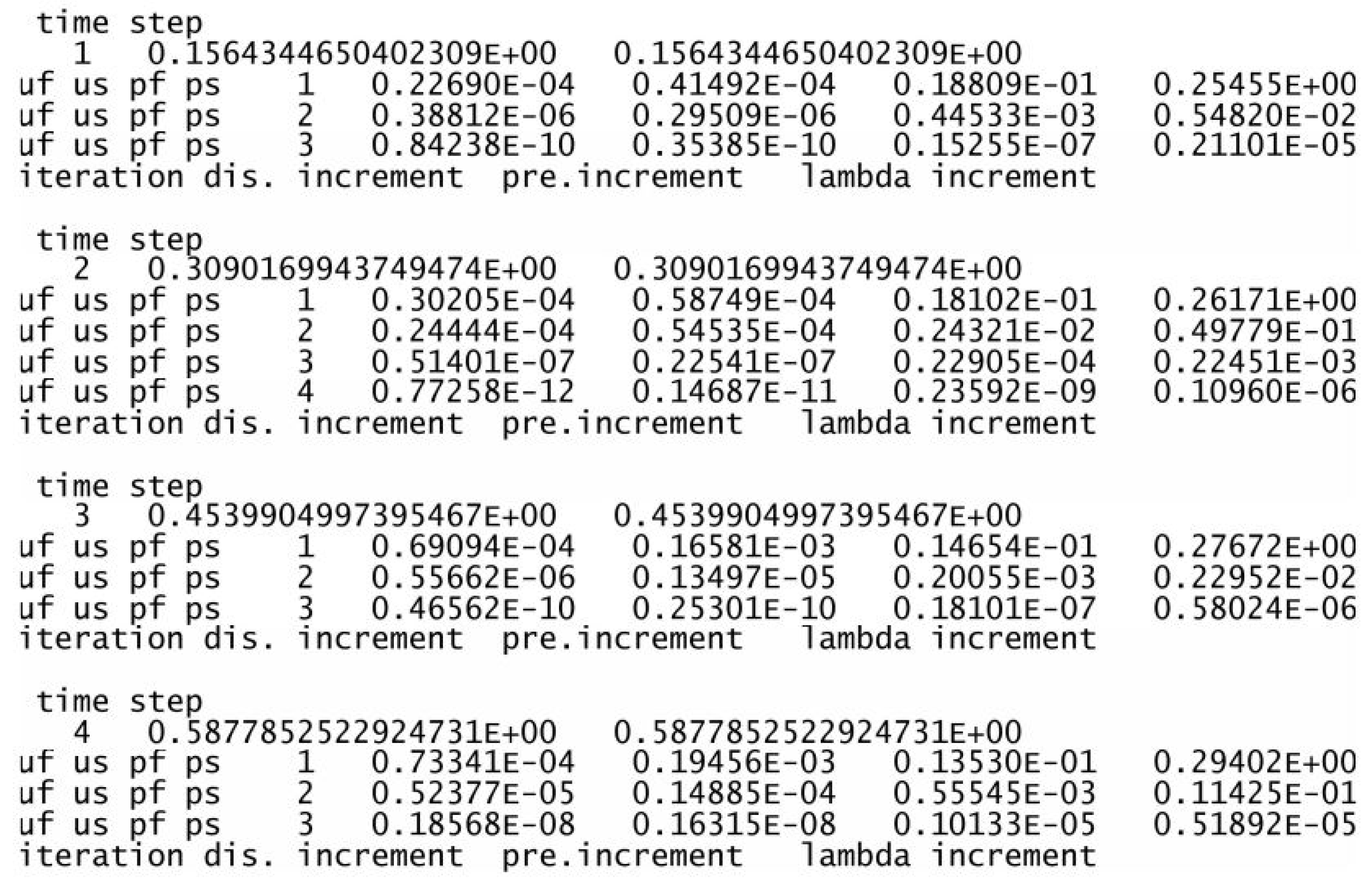
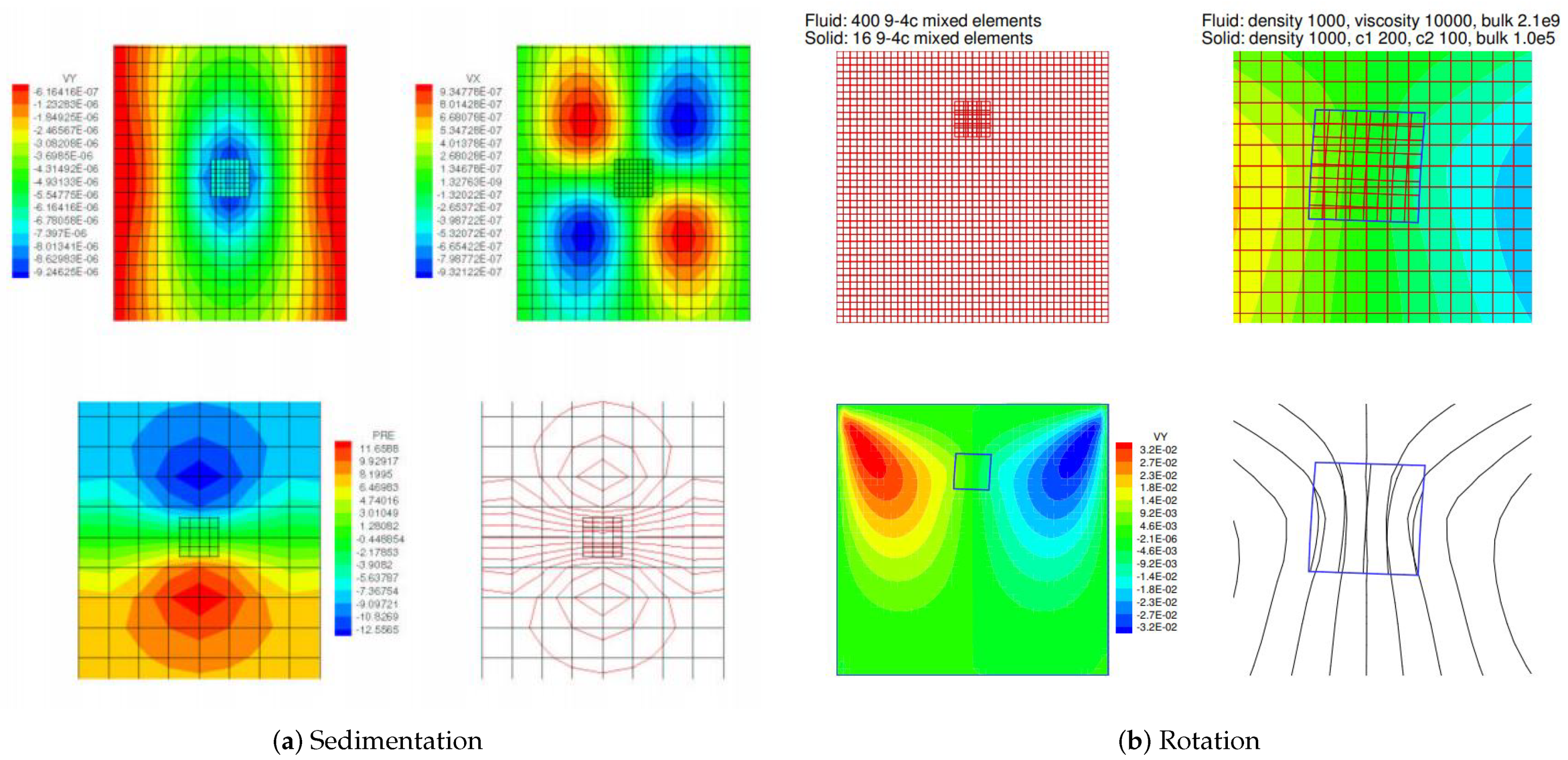
It is very important to emphasize that in this monolithic implicit matrix-free Newton–Krylov iterative solution method, the fluid velocity, the immersed solid velocity, the fluid pressure, and the solid pressure must converge simultaneously. In fact, since we obtain the immersed solid velocity based on the projection of the velocity of fluid occupying the same position, namely their simultaneously convergence is guaranteed. However, the fluid pressure and the solid pressure are calculated with two completely different procedures and the concept of addition and subtraction as illustrated in Figure 1, which ultimately marks the success of the entire monolithic implicit immersed method with matrix-free Newton–Krylov iterative solution method. As shown in Figure 12 and Figure 13, a typical converged data sheet along with two sets of pressure and velocity contour and band plots are presented for a simple sedimentation and rotation of a compressible solid in a viscous and slightly compressible fluid.
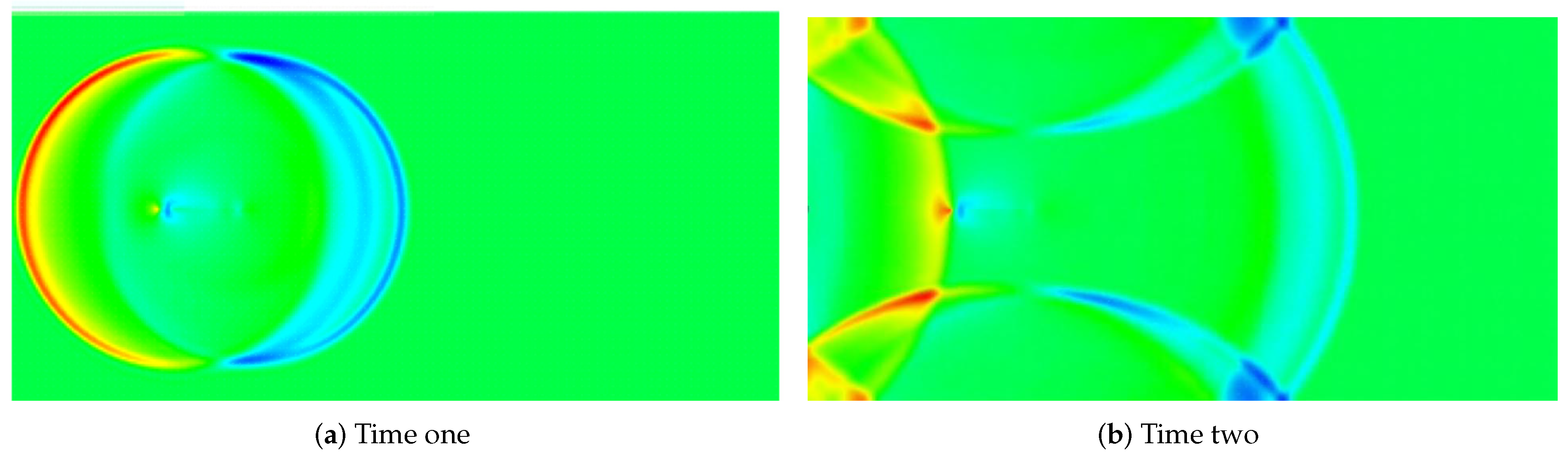
In Figure 14, we present two time snapshots taken from a case study reported in Ref. [61] in which a submerged flexible structure is interacting with the surrounding compressible fluid, more specifically, air. In this case, fully-fledged energy conservation form of governing equations in aerodynamics based on conformal mapping and compact schemes have been coupled with non-oscillatory time incremental schemes [60,61]. The specific details are imbedded in the proprietary code in Wright-Patterson Air Force Base. In order to illustrate the efficacy of immersed boundary methods for compact schemes, we intentionally set the boundaries to reflect the shock waves. It is clear that shocks are captured nicely as well as their interactions with the immersed structure.
In these implementations, we have a uniform background (ghost) mesh which allow us to employ the simple modulo function to locate the immersed solid or structure points and to implement the displacement projections and force distributions. This feature along with the concept of immersed methods enable us to avoid the topologically challenging mesh adjustments which are often prohibitive. The uniform background (ghost) mesh adopted for the compact scheme is also the important attributes for high accuracy and high computational efficiency. These features also naturally fit into parallel processing commands such as MPI and further vectorization of the operation.
6. Conclusions and Discussion
In this study, we confirm that immersed boundary methods can be applicable to compressible liquid interacting with immersed compressible solid in acoustic FSI problems. It seems equally valid for shock wave propagating in compressible fluid and acoustic waves interacting with both compressible fluid and immersed solid with the help of compact schemes.
In the monolithic implicit immersed method with Newton–Krylov iterations, in order to satisfy energy conservation, namely the energy input to the fluid domain from the immersed solid is the same as that from the equivalent body force, the same delta function must be used in both the distribution of the resultant nodal force and the interpolation of the solid velocity based on the surrounding fluid velocities. In fact, the key treatment in this fully implicit and monolithic immersed method, the synchronization of the fluid motion occupying the same geometric locations marked by the domain with the immersed solid, namely Although no explicit mathematical expression is possible in the implicit monolithic algorithms for compressible solid immersed inside a compressible fluid. However, an operator is introduced in Equation (17) to summarize such a nested fully implicit Newton–Krylov iterative procedure. In this procedure, the iterative solution based on Newton–Krylov and generalized minimal residual method (GMRES) along with the numerical construction of the Jacobian matrix in the Newton-Raphson iteration are combined as a single iterative procedure which is elaborated in detail in this paper. Furthermore, preliminary results derived with two- and three-dimensional compressible solver based on compact schemes are also included.
The constraint of Equation (42) introduces the (distributed) Lagrange multiplier as the equivalent body force. In this case, the equivalent body forces can be directly calculated along with independent fluid and solid velocity vectors. Of course, such a procedure will introduce a set of new unknowns equal to the number of velocity unknowns for solids. The early success of immersed finite element formulations for the type of immersed methods is only the beginning of this type of modeling treatment for complex FSI systems. Recent mathematical studies and extensions to electrokinetics and mass and heat transfers can also be found in Refs. [48,51].
Funding
Not Applicable.
Institutional Review Board Statement
Not Applicable.
Informed Consent Statement
Not Applicable.
Data Availability Statement
Not Applicable.
Acknowledgments
The author is very grateful for ASEE Air Force Summer Faculty Fellowship in 2008 and 2009 and the opportunity of collaboration with Raymond Gordnier, Air Vehicle Directory, Air Force Research Laboratory, WPAFB, OH 45433.
Conflicts of Interest
The author declares no conflict of interest.
References
- Belytschko, T. Fluid-structure interaction. Comput. Struct. 1980, 12, 459–469. [Google Scholar] [CrossRef]
- Liu, W.; Belytschko, T.; Chang, H. An arbitrary Lagrangian-Eulerian finite element method for path-dependent materials. Comput. Methods Appl. Mech. Eng. 1986, 58, 227–245. [Google Scholar] [CrossRef]
- Shyy, W.; Udaykumar, H.S.; Rao, M.M.; Smith, R.W. Computational Fluid Dynamics with Moving Boundaries; Taylor & Francis: London, UK, 1996. [Google Scholar]
- Wang, X.S. Fundamentals of Fluid-Solid Interactions-Analytical and Computational Approaches; Elsevier Science: Amsterdam, The Netherlands, 2008. [Google Scholar]
- Bathe, K.J.; Zhang, H.; Wang, M.H. Finite element analysis of incompressible and compressible fluid flows with free surfaces and structural interactions. Comput. Struct. 1995, 56, 193–213. [Google Scholar] [CrossRef] [Green Version]
- Bathe, K.J.; Zhang, H. Finite element developments for general fluid flows with structural interactions. Int. J. Numer. Methods Eng. 2004, 60, 213–232. [Google Scholar] [CrossRef] [Green Version]
- Tornberg, A.; Shelley, M. Simulating the dynamics and interactions of flexible fibers in stokes flows. J. Comput. Phys. 2004, 196, 8–40. [Google Scholar] [CrossRef]
- Zhang, J.; Childress, S.; Libchaber, A.; Shelley, M. Flexible filaments in a flowing soap film as a model for one-dimensional flags in a two-dimensional wind. Nature 2000, 408, 835–838. [Google Scholar] [CrossRef]
- Huerta, A.; Liu, W.K. Viscous flow with large free surface motion. Comput. Methods Appl. Mech. Eng. 1988, 69, 277–324. [Google Scholar] [CrossRef] [Green Version]
- Tezduyar, T. Stabilized finite element formulations for incompressible-flow computations. Adv. Appl. Mech. 1992, 28, 1–44. [Google Scholar]
- Tezduyar, T. Finite element methods for flow problems with moving boundaries and interfaces. Arch. Comput. Methods Eng. 2001, 8, 83–130. [Google Scholar] [CrossRef]
- Wall, W.A.; Schott, B.; Ager, C. A monolithic approach to fluid-structure interaction based on a hybrid eulerian-ALE fluid domain decomposition involving cut elements. Int. J. Numer. Methods Eng. 2019, 119, 208–237. [Google Scholar]
- Zhang, L.; Wagner, G.J.; Liu, W.K. Modeling and simulation of fluid structure interaction by meshfree and FEM. Commun. Numer. Methods Eng. 2003, 19, 615–621. [Google Scholar] [CrossRef]
- Oshe, S.J.; Fedki, R.P. Level Set Methods and Dynamic Implicit Surfaces; Springer: Berlin/Heidelberg, Germany, 2002. [Google Scholar]
- Sethian, J.A. Level Set Methods and Fast Marching Methods; Cambridge University Press: Cambridge, UK, 1996. [Google Scholar]
- LeVeque, R.; Li, Z. Immersed interface methods for Stokes flow with elastic boundaries or surface tension. SIAM J. Sci. Comput. 1997, 18, 709–735. [Google Scholar] [CrossRef] [Green Version]
- Li, Z.; LeVeque, R. The immersed interface methods for elliptic equations with discontinuous coefficients and singular sources. SIAM J. Sci. Comput. 1994, 31, 1019–1044. [Google Scholar]
- Glimm, J.; Grove, J.W.; Li, X.L.; Tan, D.C. Robust computational algorithms for dynamic interface tracking in three dimensions. SIAM J. Sci. Comput. 2000, 21, 2240–2256. [Google Scholar] [CrossRef]
- Li, X.L.; Jin, B.X.; Glimm, J. Numerical study for the three-dimensional Rayleigh-Taylor instability through the TVD/AC scheme and parallel computation. J. Comput. Phys. 1996, 126, 343–355. [Google Scholar] [CrossRef] [Green Version]
- Tryggvason, G. Numerical simulations of the Rayleigh-Taylor instability. J. Comput. Phys. 1988, 75, 253–282. [Google Scholar] [CrossRef] [Green Version]
- Farhat, C.; Geuzaine, P.; Grandmont, C. The discrete geometric conservation law and the nonlinear stability of ALE schemes for the solution of flow problems on moving grids. J. Comput. Phys. 2001, 174, 669–694. [Google Scholar] [CrossRef]
- Hughes, T.; Liu, W.K.; Zimmerman, T.K. Lagrangian-Eulerian finite element formulations for incompressible viscous flows. Comput. Methods Appl. Mech. Eng. 1981, 29, 329–349. [Google Scholar] [CrossRef]
- Kamakoti, R.; Shyy, W. Fluid-structure interaction for aeroelastic applications. Prog. Aerosp. Sci. 2004, 40, 535–558. [Google Scholar] [CrossRef]
- Lian, Y.; Shyy, W. Numerical simulations of membrane wing aerodynamics for micro air vehicle applications. J. Aircr. 2005, 42, 865–873. [Google Scholar] [CrossRef]
- Shyy, W.; Berg, M.; Ljungqvist, D. Flapping and flexible wings for biological and micro air vehicles. Prog. Aerosp. Sci. 1999, 35, 455–505. [Google Scholar] [CrossRef]
- Chessa, J.; Belytschko, T. The extended finite element method for two-phase fluids. J. Appl. Mech. 2003, 70, 10–17. [Google Scholar] [CrossRef]
- Wagner, G.; Moës, N.; Liu, W.K.; Belytschko, T. The extended finite element method for rigid particles in stokes flow. Int. J. Numer. Methods Eng. 2001, 51, 293–313. [Google Scholar] [CrossRef]
- Glowinski, R.; Pan, T.; Hesla, T.I.; Joseph, D.D.; Périaux, J. A fictitious domain approach to the direct numerical simulation of incompressible viscous flow past moving rigid bodies: Application to particulate flow. J. Comput. Phys. 2001, 169, 363–426. [Google Scholar] [CrossRef] [Green Version]
- Wang, X.; Yang, Y.; Wu, T. Model studies of fluid-structure interaction problems. Comput. Model. Eng. Sci. 2019, 119, 5–34. [Google Scholar]
- McQueen, D.; Peskin, C. Computer-assisted design of butterfly bileaflet valves for the mitral position. Scand. J. Thor. Cardiovasc. Surg. 1985, 19, 139–148. [Google Scholar] [CrossRef] [PubMed]
- Peskin, C. Numerical analysis of blood flow in the heart. J. Comput. Phys. 1977, 25, 220–252. [Google Scholar] [CrossRef]
- Peskin, C. The immersed boundary method. Acta Numer. 2002, 11, 479–517. [Google Scholar] [CrossRef] [Green Version]
- Beyer, R. A computational model of the cochlea using the immersed boundary method. J. Comput. Phys. 1992, 98, 145–162. [Google Scholar] [CrossRef]
- Fauci, L.; Peskin, C. A computational model of aquatic animal locomotion. J. Comput. Phys. 1988, 77, 85–108. [Google Scholar] [CrossRef]
- Stockie, J.M.; Wetton, B.R. Analysis of stiffness in the immersed boundary method and implications for time-stepping schemes. J. Comput. Phys. 1999, 154, 41–64. [Google Scholar] [CrossRef] [Green Version]
- Dillon, R.; Fauci, L.; Fogelson, A.; Gaver, D., III. Modeling biofilm processes using the immersed boundary method. J. Comput. Phys. 1996, 129, 57–73. [Google Scholar] [CrossRef]
- van Loon, R.; Anderson, P.D.; van de Vosse, F.N.; Sherwin, S.J. Comparison of various fluid-structure interaction methods for deformable bodies. Comput. Struct. 2007, 85, 833–843. [Google Scholar] [CrossRef] [Green Version]
- Yu, Z. A DLM/FD method for fluid/flexible-body interactions. J. Comput. Phys. 2005, 207, 1–27. [Google Scholar] [CrossRef]
- Wang, X.; Zhang, L.T.; Liu, W.K. On computational issues of immersed finite element methods. J. Comput. Phys. 2009, 228, 2535–2551. [Google Scholar] [CrossRef]
- Sulsky, D.; Kaul, A. Implicit dynamics in the material-point method. Comput. Methods Appl. Mech. Eng. 2004, 193, 1137–1170. [Google Scholar] [CrossRef]
- Lim, S.; Ferent, A.; Wang, X.; Peskin, C. Dynamics of a closed rod with twist and bend in fluid. SIAM J. Sci. Comput. 2008, 31, 273–302. [Google Scholar] [CrossRef]
- Gay, M.; Zhang, L.T.; Liu, W.K. Stent modeling using immersed finite element method. Comput. Methods Appl. Mech. Eng. 2005, 195, 4358–4370. [Google Scholar] [CrossRef]
- Liu, W.; Liu, Y.; Farrell, D.; Zhang, L.; Wang, X.; Fukui, Y.; Patankar, N.; Zhang, Y.; Bajaj, C.; Chen, X.; et al. Immersed finite element method and its applications to biological systems. Comput. Methods Appl. Mech. Eng. 2006, 195, 1722–1749. [Google Scholar] [CrossRef] [PubMed] [Green Version]
- Liu, W.; Jun, S.; Zhang, Y.F. Reproducing kernel particle methods. Int. J. Numer. Methods Fluids 1995, 20, 1081–1106. [Google Scholar] [CrossRef]
- Boffi, D.; Gastaldi, L. A finite element approach for the immersed boundary method. Comput. Struct. 2003, 81, 491–501. [Google Scholar] [CrossRef]
- Mori, Y.; Peskin, C. Implicit second-order immersed boundary methods with boundary mass. Comput. Methods Appl. Mech. Eng. 2008, 197, 2049–2067. [Google Scholar] [CrossRef]
- Newren, E.; Fogelson, A.L.; Guy, R.D.; Kirby, R.M. Unconditionally stable discretizations of the immersed boundary equations. J. Comput. Phys. 2007, 222, 702–719. [Google Scholar] [CrossRef]
- Liu, Y.; Liu, W.K.; Belytschko, T.; Patankar, N.; To, A.C.; Kopacz, A.; Chung, J.H. Immersed electrokinetic finite element method. Int. J. Numer. Methods Eng. 2007, 71, 379–405. [Google Scholar] [CrossRef]
- Liu, Y.; Zhang, L.; Wang, X.; Liu, W.K. Coupling of Navier-Stokes equations with protein molecular dynamics and its application to hemodynamics. Int. J. Numer. Methods Fluids 2004, 46, 1237–1252. [Google Scholar] [CrossRef]
- Fogelson, A.; Wang, X.; Liu, W.K. Special issue: Immersed boundary method and its extensions—Preface. Comput. Methods Appl. Mech. Eng. 2008, 197, 25–28. [Google Scholar]
- Liu, W.; Kim, D.W.; Tang, S. Mathematical foundations of the immersed finite element method. Comput. Mech. 2007, 39, 211–222. [Google Scholar] [CrossRef]
- Mittal, R.; Iaccarino, G. Immersed boundary methods. Annu. Rev. Fluid Mech. 2005, 37, 239–261. [Google Scholar] [CrossRef] [Green Version]
- Wang, X. From immersed boundary method to immersed continuum method. Int. J. Multiscale Comput. Eng. 2006, 4, 127–145. [Google Scholar] [CrossRef]
- Wang, X. An iterative matrix-free method in implicit immersed boundary/continuum methods. Comput. Struct. 2007, 85, 739–748. [Google Scholar] [CrossRef]
- Sulsky, D.; Brackbill, J.U. A numerical method for suspension flow. J. Comput. Phys. 1991, 96, 339–368. [Google Scholar] [CrossRef]
- Boffi, D.; Gastaldi, L.; Heltai, L. On the CFL condition for the finite element immersed boundary method. Comput. Struct. 2007, 85, 775–783. [Google Scholar] [CrossRef]
- Boffi, D.; Gastaldi, L.; Heltai, L.; Peskin, C. On the hyperelastic formulation of the immersed boundary method. Comput. Methods Appl. Mech. Eng. 2008, 197, 2210–2231. [Google Scholar] [CrossRef]
- Wang, X.; Liu, W.K. Extended immersed boundary method using FEM and RKPM. Comput. Methods Appl. Mech. Eng. 2004, 193, 1305–1321. [Google Scholar] [CrossRef]
- Zhang, L.; Gerstenberger, A.; Wang, X.; Liu, W.K. Immersed finite element method. Comput. Methods Appl. Mech. Eng. 2004, 193, 2051–2067. [Google Scholar] [CrossRef]
- Shu, C.W. Essential non-oscillatory and weighted essentially non-oscillatory schemes. Acta Numer. 2020, 1–60. [Google Scholar]
- Wang, X.; Gordnier, R. A combination of immersed methods and compact scheme based computational fluid dynamics for fluid-structure interactions. In Air Force ASEE Summer Faculty Fellow Report; Midwestern State University: Wichita Falls, TX, USA, 2009. [Google Scholar]
- Wang, X.; Bathe, K.J. Displacement/pressure based finite element formulations for acoustic fluid-structure interaction problems. Int. J. Numer. Methods Eng. 1997, 40, 2001–2017. [Google Scholar] [CrossRef]
- Wang, X.; Bathe, K.J. On mixed elements for acoustic fluid-structure interactions. Math. Model. Methods Appl. Sci. 1997, 7, 329–343. [Google Scholar] [CrossRef]
- Bao, W.; Wang, X.; Bathe, K.J. On the Inf-Sup condition of mixed finite element formulations for acoustic fluids. Math. Model. Methods Appl. Sci. 2001, 11, 883–901. [Google Scholar] [CrossRef] [Green Version]
- Bathe, K. Finite Element Procedures; Prentice Hall: Englewood Cliffs, NJ, USA, 1996. [Google Scholar]
- Li, S.; Liu, W.K. Reproducing kernel hierarchical partition of unity part I: Formulation and theory. Int. J. Numer. Methods Eng. 1999, 45, 251–288. [Google Scholar] [CrossRef]
- Liu, W.; Chen, Y.; Chang, C.T.; Belytschko, T. Advances in multiple scale kernel particle methods. Comput. Mech. 1996, 18, 73–111. [Google Scholar] [CrossRef]
- Liu, W.; Chen, Y.; Uras, R.A.; Chang, C.T. Generalized multiple scale reproducing kernel particle methods. Comput. Methods Appl. Mech. Eng. 1996, 139, 91–157. [Google Scholar] [CrossRef]
- Liu, W.; Chen, Y.J. Wavelet and multiple scale reproducing kernel methods. Int. J. Numer. Methods Fluids 1995, 21, 901–932. [Google Scholar] [CrossRef]
- Wang, X. On the discretized delta function and force calculation in the immersed boundary method. In Computational Fluid and Solid Mechanics; Bathe, K., Ed.; Elsevier: Amsterdam, The Netherlands, 2003; pp. 2164–2169. [Google Scholar]
- Griffith, B.; Patankar, N.A. Immersed methods for fluid-structure interaction. Annu. Rev. Fluid Mech. 2020, 52, 421–448. [Google Scholar] [CrossRef] [PubMed] [Green Version]
- Wang, X.; Zhang, L. Immersed Methods for Coupled Systems of Continua; World Scientific Publishing Co.: Singapore, 2021. [Google Scholar]
- Pan, T. Private Communications. 2021. Available online: http://www.math.uh.edu/ (accessed on 4 May 2021).
- Vincent, S.; Caltagirone, J.P. A monolithic approach of fluid–structure interaction by discrete mechanics. Fluids 2021, 6, 95. [Google Scholar] [CrossRef]
Figure 1.
The concept of fictitious fluid domain vs. immersed domain.

Figure 2.
An illustration of a Lagrangian mesh on top of a Eulerian mesh for immersed methods.

Figure 3.
Pressure distribution of an acoustic fluid-solid interaction system (from the author’s earlier work [29,62,63]).

Figure 4.
A comparison of various discretized delta functions and their spectra (from the author’s earlier work [58,70]).

Figure 5.
One-dimensional model problem of one continuum immersed in another continuum.

Figure 6.
Analytical solutions.

Figure 7.
Comparisons with the monolithic implicit immersed method with matrix-free Newton–Krylov iterations and ADINA.
Figure 7.
Comparisons with the monolithic implicit immersed method with matrix-free Newton–Krylov iterations and ADINA.

Figure 8.
Snapshots of results from the immersed continuum method and the ADINA FSI solver.

Figure 9.
A comparison of horizontal and vertical velocities derived from the traditional ALE formulation and the immersed methods.
Figure 9.
A comparison of horizontal and vertical velocities derived from the traditional ALE formulation and the immersed methods.

Figure 10.
Extra numerical dissipation due to immersed methods.

Figure 11.
Driven cavity with five compressible immersed solids.

Figure 12.
Simultaneous convergence of the monolithic implicit immersed method with matrix-free Newton– Krylov iteration.
Figure 12.
Simultaneous convergence of the monolithic implicit immersed method with matrix-free Newton– Krylov iteration.

Figure 13.
Fully converged velocity and pressure contours and bandplots.

Figure 14.
Shockwave propagating within compressible air with compact schemes (from the author’s earlier work Ref. [61]).
Figure 14.
Shockwave propagating within compressible air with compact schemes (from the author’s earlier work Ref. [61]).

Publisher’s Note: MDPI stays neutral with regard to jurisdictional claims in published maps and institutional affiliations. |
© 2021 by the author. Licensee MDPI, Basel, Switzerland. This article is an open access article distributed under the terms and conditions of the Creative Commons Attribution (CC BY) license (https://creativecommons.org/licenses/by/4.0/).
Share and Cite
MDPI and ACS Style
Wang, S. A Revisit of Implicit Monolithic Algorithms for Compressible Solids Immersed Inside a Compressible Liquid. Fluids 2021, 6, 273. https://0-doi-org.brum.beds.ac.uk/10.3390/fluids6080273
AMA Style
Wang S. A Revisit of Implicit Monolithic Algorithms for Compressible Solids Immersed Inside a Compressible Liquid. Fluids. 2021; 6(8):273. https://0-doi-org.brum.beds.ac.uk/10.3390/fluids6080273
Chicago/Turabian StyleWang, Sheldon. 2021. "A Revisit of Implicit Monolithic Algorithms for Compressible Solids Immersed Inside a Compressible Liquid" Fluids 6, no. 8: 273. https://0-doi-org.brum.beds.ac.uk/10.3390/fluids6080273