
Correlation between Large-Scale Streamwise Velocity Features and the Height of Coherent Vortices in a Turbulent Boundary Layer


1
Indian Institute of Technology, Kharagpur 721302, India
2
Department of Aerospace Engineering, University of Illinois at Urbana-Champaign, Urbana, IL 61801, USA
*
Author to whom correspondence should be addressed.
Fluids 2021, 6(8), 286; https://0-doi-org.brum.beds.ac.uk/10.3390/fluids6080286
Submission received: 30 June 2021
/
Revised: 6 August 2021
/
Accepted: 10 August 2021
/
Published: 16 August 2021
(This article belongs to the Special Issue Turbulent Flows at Solid and Free Surface Boundaries in Memory of William W. Willmarth)
Abstract
:The preferential organisation of coherent vortices in a turbulent boundary layer in relation to local large-scale streamwise velocity features was investigated. Coherent vortices were identified in the wake region using the Triple Decomposition Method (originally proposed by Kolář) from 2D particle image velocimetry (PIV) data of a canonical turbulent boundary layer. Two different approaches, based on conditional averaging and quantitative statistical analysis, were used to analyze the data. The large-scale streamwise velocity field was first conditionally averaged on the height of the detected coherent vortices and a change in the sign of the average large scale streamwise fluctuating velocity was seen depending on the height of the vortex core. A correlation coefficient was then defined to quantify this relationship between the height of coherent vortices and local large-scale streamwise fluctuating velocity. Both of these results indicated a strong negative correlation in the wake region of the boundary layer between vortex height and large-scale velocity. The relationship between vortex height and full large-scale velocity isocontours was also studied and a conceptual model based on the findings of the study was proposed. The results served to relate the hairpin vortex model of Adrian et al. to the scale interaction results reported by Mathis et al., and Chung and McKeon.
1. Introduction
Coherent motions in wall turbulence have been treated in detail in various reviews [1,2]. Coherent vortex structures or ‘eddies’, including horseshoe or hairpin vortices were first proposed as a key turbulent feature in 1952 [3] and were later experimentally observed [4]. The structural organisation of vortex structures and their position relative to large-scale velocity structures in wall-bounded turbulence has been a topic of interest for decades. Falco [5] identified vortices at the upstream border of large-scale bulges in the velocity field. Groups of vortices in the logarithmic and wake regions of wall-bounded turbulent flows have been associated with low-momentum regions and ejection motions, including in the attached eddy model of Perry and Chong [6], the hairpin packet model of Adrian et al. [7], and the vortex clusters observed by Lozano-Durán et al. [8]. The ‘attached eddy model’ (AEM) used wall-attached hierarchies of groups of arch-like or hairpin vortex structures with ejections beneath them to represent turbulent wall-bounded flows [6]. de Silva et al. [9] used the AEM to generate synthetic datasets of turbulent boundary layer and study the distribution of Uniform Momentum Zones (UMZs) in the wake region. Recent work focused on incorporating the experimental observations into the synthetic AEMs ([10,11]), which improved replication of instantaneous features. In the hairpin packet perspective, arch-like vortices generate low momentum flow beneath them due to vortex induction. Hairpin vortices have been visualized in particle image velocimetry and large-eddy simulation data and have been shown to generate other hairpin vortices in computational experiments [2,7,12]. In the vortex cluster perspective, vortices are not restricted to an arch-like shape and can instead be chaotically shaped [8]. Lozano-Durán et al. [8] suggested that the vortex clusters were generated from the large-scale velocity structures, rather than driving the large-scale velocity structure generation. Whether true arch-like or hairpin vortices persist at higher Reynolds numbers is a topic of continued debate [13,14], and discrepancies between observed vortex structures from experimentalists and computationalists might be explainable by the scale of the vortex structures that are being considered [15]. Regardless of the precise shape of the vortex structure, the passage of a coherent vortex or groups of vortices has been shown to consistently correlate with bursting motions in wall-bounded turbulent flows [5,16]. Heisel et al. [17] found that vortices generally aligned with thin concentrations of shear called internal shear layers or vortical fissures [18,19,20].
Large-scale velocity structures and their influence on other scales have also been characterized in turbulent boundary layers independently of vortex structures. Very-large-scale motions (VLSMs) and large-scale motions (LSMs) have been identified from streamwise velocity spectra of pipe, channel, and boundary layer flows [21]. VLSMs meander in the log-layer with a length of approximately 6–10 times the outer length scale [22]. LSMs dominate the wake region with a length of approximately 2–4 times the outer length scale [21]. In the near-wall region, near-wall streaks and streamwise vortices dominate the flow [23,24] and sustain autonomously, without needing the influence of the outer region [25]. However, the VLSMs do influence the near-wall region; in Mathis et al. [26], the authors found that the large scales impose an amplitude modulating effect on the small scales in a turbulent boundary layer. The authors defined a new term, a correlation coefficient, to study the correlation between large scales and the envelope of small scales. The velocity signals were sampled and filtered to separate the large and small scales and the Hilbert Transform was employed to capture the envelope of the small scales. The correlation coefficient was found to vary from strongly positive peak in the near-wall region to strongly negative in the wake region, with a zero crossing in the logarithmic layer. In Bernardini and Pirozzoli [27], the authors suggested a modified definition of correlation coefficient using a two-point correlation, thus allowing giving a more refined estimation of the amplitude modulation phenomenon. Baars et al. [28] observed that small-scale fluctuations were enhanced or weakened subject to the local large-scale structures across many Reynolds numbers. Chung and McKeon [29] used conditional averaging and a box filter to study the effect of LSMs and VLSMs on small scales, and found stronger small scales farther from the wall in the presence of large-scale low-speed events and nearer to the wall in the presence large-scale high-speed events in the logarithmic and wake regions of a turbulent boundary layer using large-eddy simulation data.
This paper seeks to identify how the height that coherent vortices appear in a flow field is correlated to the amplitude of large-scale velocity events in the wake region of turbulent boundary layers. The work seeks to connect the vortex-based coherent structure models to the amplitude modulation data. Methods used to identify coherent vortices in turbulent boundary layer data and to filter large-scale velocity signals from the raw velocity information are provided in Section 2. Large-scale velocity fields, conditioned on the height of identified coherent vortices, a new correlation coefficient, and the distance between the vortex heights and the large-scale velocity isocontours are presented in Section 3. Finally, the results are discussed and summarized in Section 4.
2. Methods
2.1. Data Source
Particle image velocimetry (PIV) was used to acquire velocity data in the wall-normal (y)—streamwise (x) plane for a turbulent boundary layer flow over a flat-plate, with a , where is the friction velocity approximated using a Clauser method, is the 99% boundary layer thickness and is the kinematic viscosity. Data were collected at a frequency of 1.5 kHz with a velocity vector every 14 viscous units, normalized by and . More details of the experimental set up can be found in Saxton-Fox and McKeon [30].
2.2. Vortex Identification
The Triple Decomposition Method (TDM) was used to identify coherent spanwise vorticity in the data set. TDM distinguishes shearing, straining, and swirling motions by decomposing the velocity gradient tensor into three parts [31],
where the subscript stands for the elongation part, the subscript stands for rigid body rotation, and the subscript stands for pure shearing motion. This decomposition can be rewritten as
which can then be expressed as
After a few mathematical manipulations, the residual vorticity can be defined as the difference between planar vorticity and strain-rate magnitude,
In comparison, the square of swirling strength magnitude can be expressed as,
The TDM gives a better approximation of the vortex rotation, especially when the vortex is under shear, compared to swirling strength [31]. In this study, we use the residual vorticity as our primary parameter for identifying a coherent vortex.
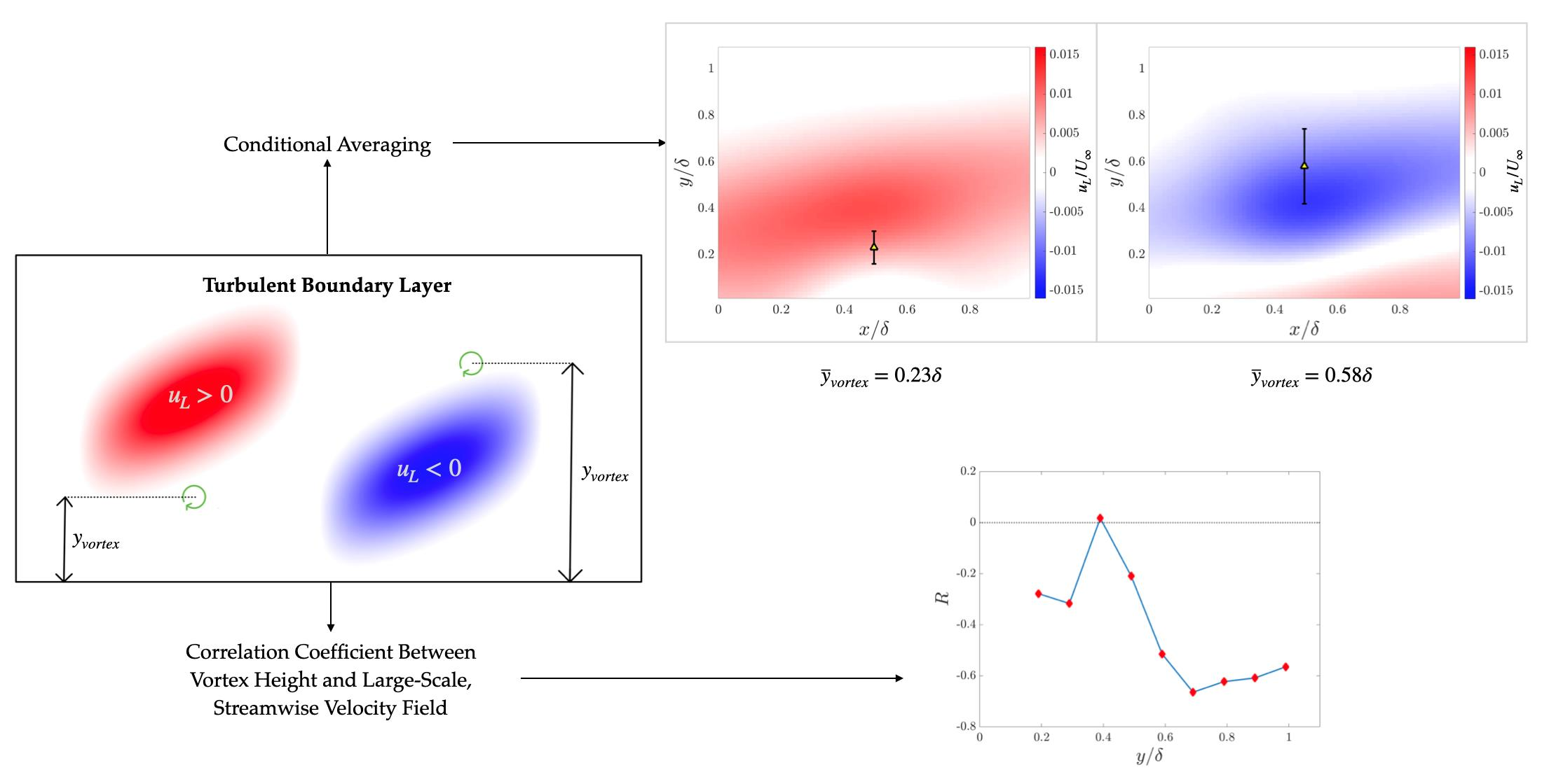
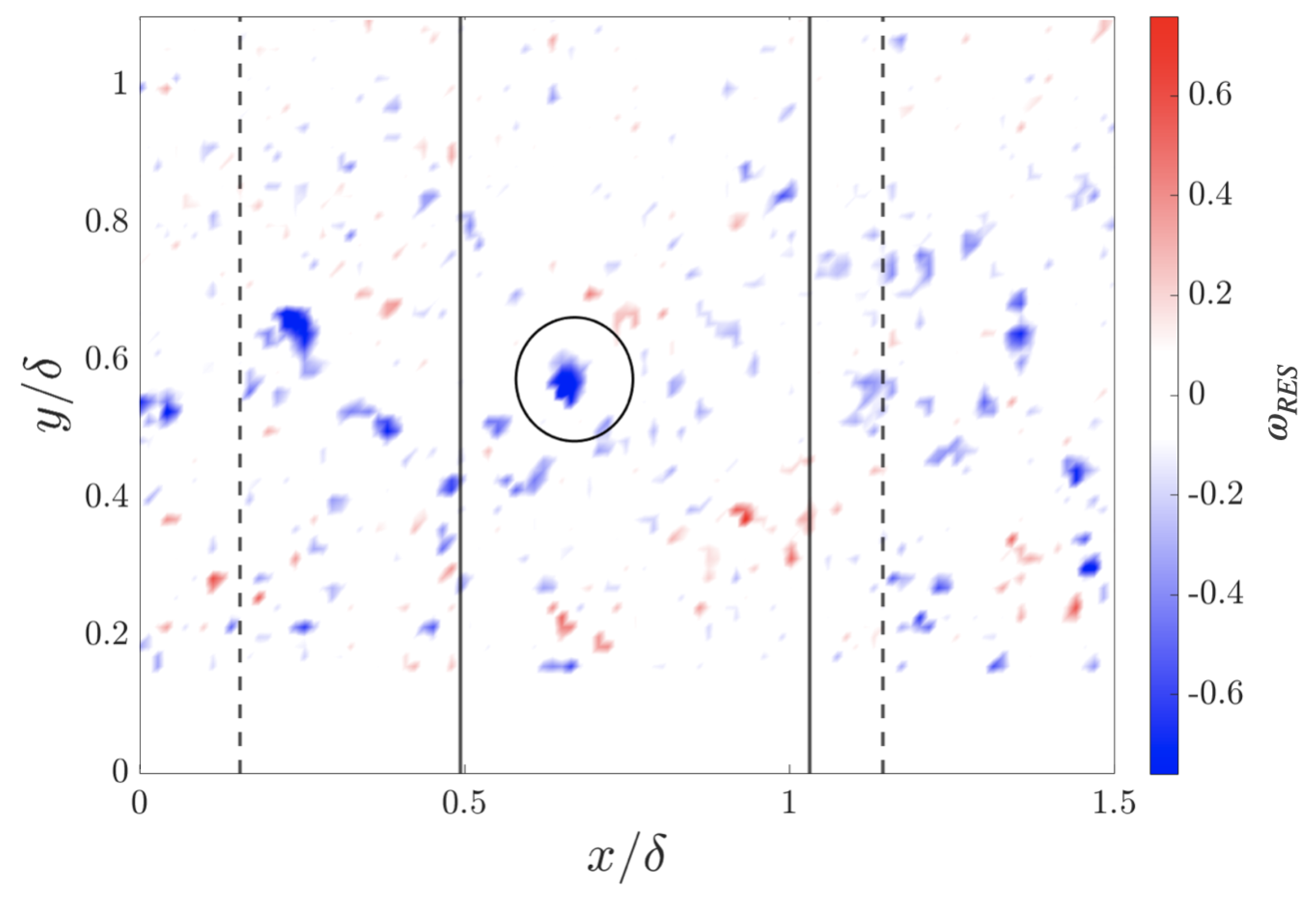
Figure 1 shows the vector field map of the planar residual vorticity, The red (blue) areas in the plot indicate peaks in with anticlockwise (clockwise) rotations, indicating the presence of a vortex. The presence of a vortex is confirmed in Figure 2, where the velocity is plotted with respect to a moving reference frame with for the same snapshot. The rectangle in the figure highlights the region where the TDM predicted the vortex location.
A vortex was defined as a region with a strong local peak in the magnitude of residual vorticity . A subset of strong spanwise vortices were the focus of this study. To select this subset, the strongest spanwise vortex in a two-dimensional plane with a streamwise length of 1 and a wall-normal height between was identified. The strongest such vortex in each snapshot was recorded and its characteristics studied. The height of a vortex was defined as the wall-normal coordinate of the point at which the residual vorticity of the strongest local vortex reached a local maximum. In this study, only vortices above a height were considered, allowing the study to focus on the wake region. Future work will focus on the logarithmic region of the boundary layer.
2.3. Filtering
The large-scale velocity field was defined by convolving the velocity field with a Gaussian function, which was chosen due to its smooth behavior in both physical and Fourier space. The standard deviation of the Gaussian function was chosen to be , where is the boundary layer thickness, which corresponded to an approximate cutoff frequency . The fluctuating large-scale streamwise velocity field was defined as and the non-fluctuating large-scale streamwise velocity field was defined as . A small-scale streamwise velocity field was defined as .
The large-scale velocity fields were sampled such that the relevant vortex was always at the center of the sampled velocity field and the streamwise width of the sampled large-scale velocity field was equal to . These individual large-scale velocity fields were then conditionally averaged on the height of the vortex. The sampling region for the large-scale velocity field is shown as dashed lines in Figure 1.
2.4. Relationship between Coherent Vortices and Small-Scale Velocity Features
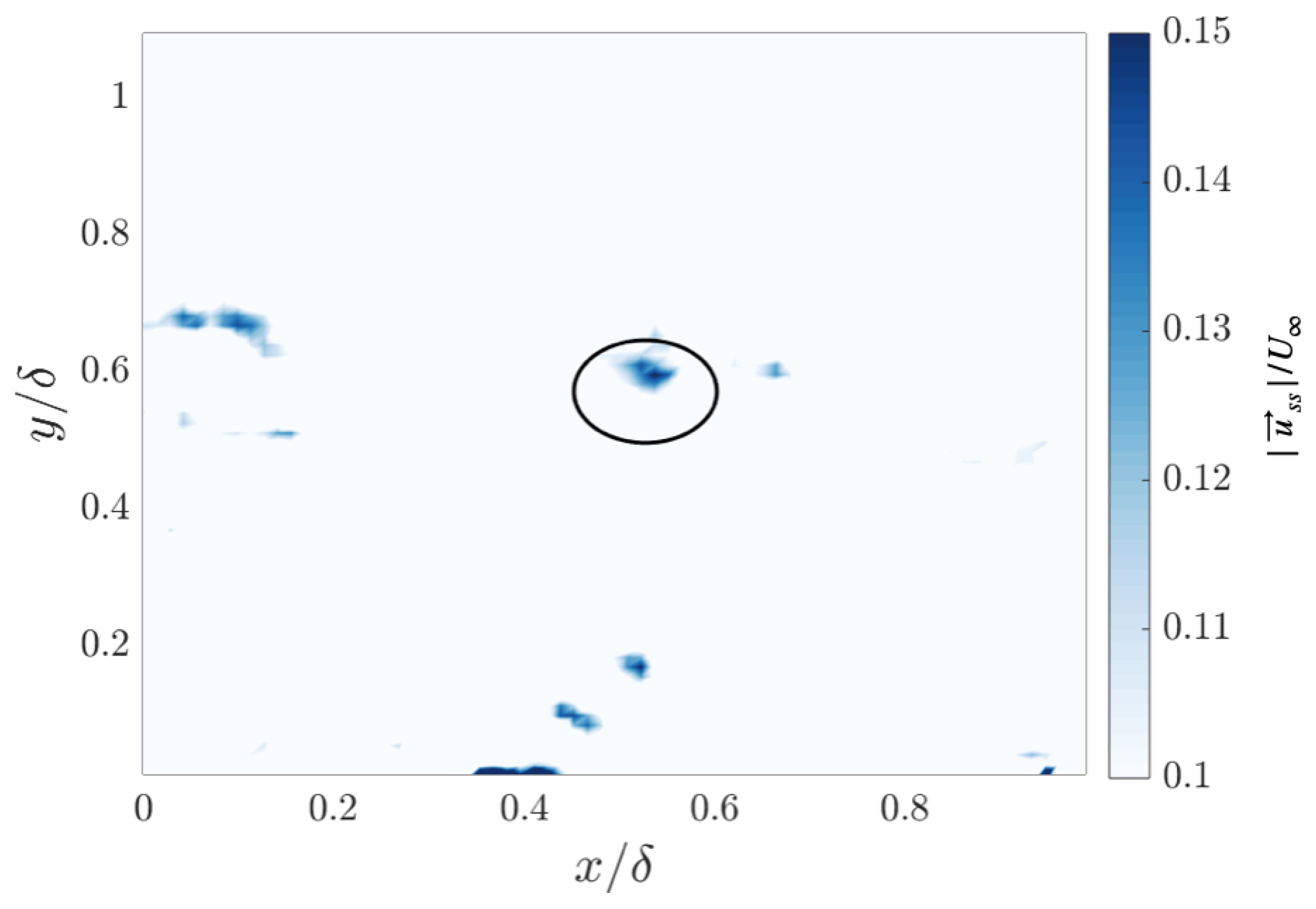
To connect the results of this paper to the amplitude modulation results of Mathis et al. [26] and the conditional averaging results of Chung and McKeon [29], the relationship between coherent vortices and local small scale velocity features is highlighted. Figure 3 shows the contour plot of magnitude of fluctuating small-scale velocity field. The ellipse in the figure indicates the location of the identified vortex. A strong peak in the small-scale velocity magnitude is observed near the location of the identified vortex, which signifies a direct correlation between small-scale velocity features and the coherent vortices used in this study.
3. Results
3.1. Conditional Averaging
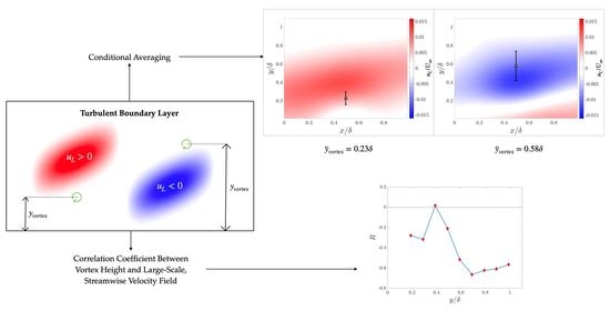
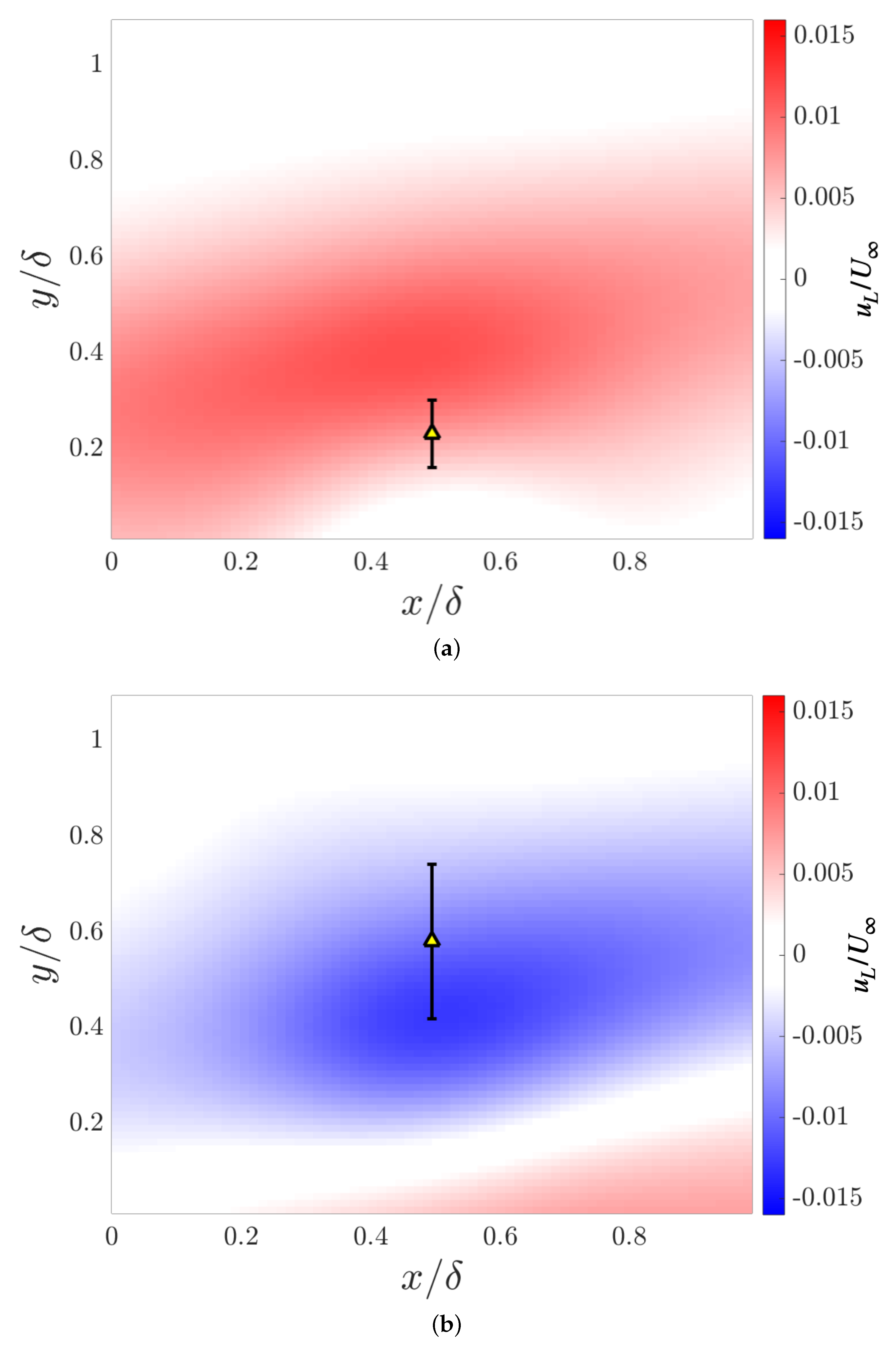
The mean height of all the identified coherent vortices was found to be . We define the relative height of the vortex as . The fluctuating large-scale velocity field was averaged separately for and , and the results are shown in Figure 4. When the coherent vortices were nearer to the wall, the large-scale velocity field was dominated by high-speed streamwise velocity, as shown in Figure 4a, while when the vortices were farther away from the wall, the large-scale velocity field was dominated by low-speed streamwise velocity, as shown in Figure 4b, The averaging was performed for 759 and 521 snapshots for and respectively. The number of vortices was observed to be higher near the wall than farther away from the wall, which agrees with the attached eddy model of Perry and Chong [6]. A more detailed analysis of the distribution of number of vortices against wall-normal height has been presented in Appendix A.
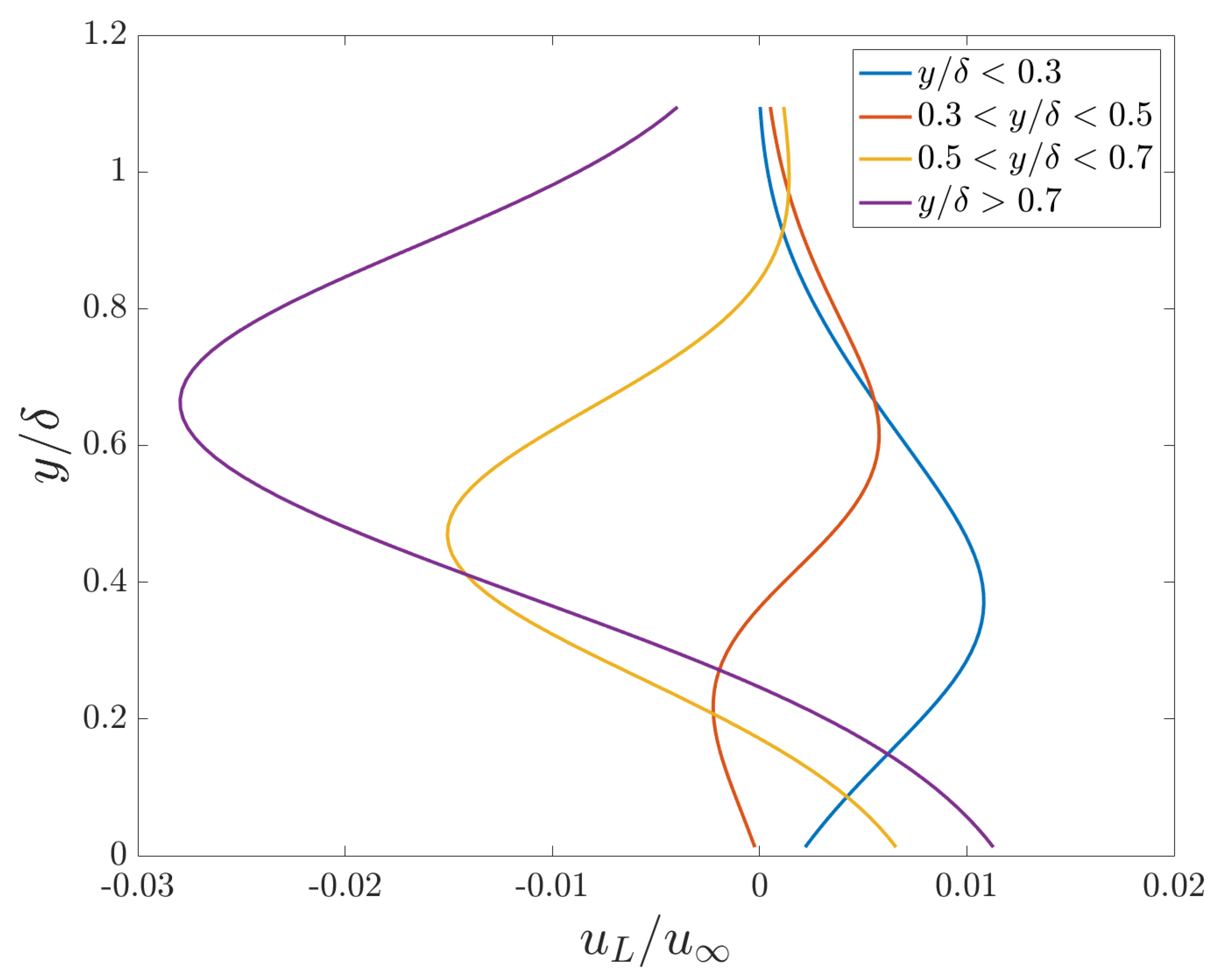
To further study correlation between the large-scale structures and the spatial location of the coherent vortices, the vortex heights were binned into four different ranges, (a) , (b) , (c) , and, (d) . For each snapshot, the fluctuating large-scale velocity field was first spatially averaged in the streamwise direction. The spatially averaged fluctuating large-scale velocity profile as a function of normalised distance from the wall, , was then averaged temporally in each of the four bins. The results are shown in Figure 5. When the coherent vortices are close to the wall, as in case (a) of Figure 5, shown in a blue curve, the fluctuating large-scale velocity profile is largely positive and has a peak in magnitude close to the wall. The fluctuating large-scale velocity profile is instead largely negative for cases (c) and (d) of Figure 5 (yellow and purple curves), when the coherent vortices are farther from the wall. In these cases, the fluctuating streamwise large-scale velocity peak is increasingly far from the wall. The peaks are stronger when the vortex is closest to or farthest from the wall. Case (b) of Figure 5 (red curve) shows both positive and negative large-scale streamwise fluctuating velocity, with a negative peak nearer to the wall and a positive peak farther from the wall.
3.2. Correlation Coefficient
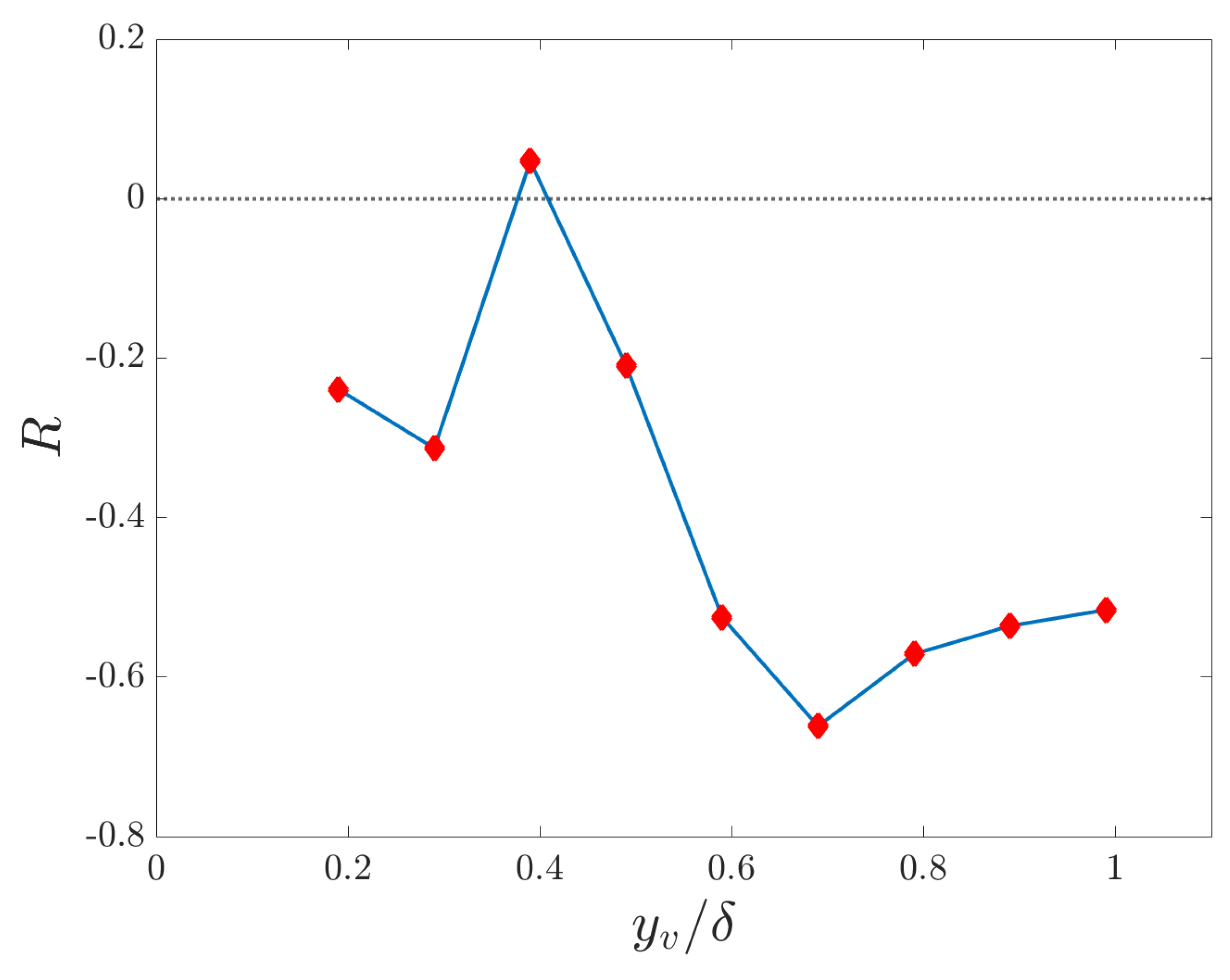
A Pearson correlation coefficient, R, was used to quantify the relationship between the height of a coherent vortex and the fluctuating large-scale streamwise velocity field. The correlation coefficient is defined in (7), where denotes the root mean square of the relative vortex height, , and .
In this definition, is the local fluctuating large-scale streamwise velocity sampled at the same streamwise location as that of the identified vortex, , but at a constant height, . For this study, the constant height is shown at ; very little sensitivity was found when this height was adjusted within the heights of the wake region. The vortex heights were binned in values of , where the height of the vortices varied from to . Mean correlation values were calculated for each bin and plotted as a function of normalised height of the vortex . The results are plotted as shown in Figure 6.
The correlation coefficient is negative in almost all of the bins. Because of the subtraction of the mean from the height of the vortex, the correlation is close to zero around the mean height, , which is expected. For heights farther away from the wall, the correlation is more negative and peaks at . Closer to the wall, the correlation value remained near −0.2. The flow nearer to the wall, where , was not studied; the physics of the wake region were the focus of this work. Future work will consider the organization of the logarithmic region.
The correlation coefficient was also calculated without binning by ranges of vortex height. When calculated for more than 5000 snapshots, the mean correlation coefficient over all ranges of vortex heights was found to be .
3.3. Relationship to Large-Scale Velocity Isocontour
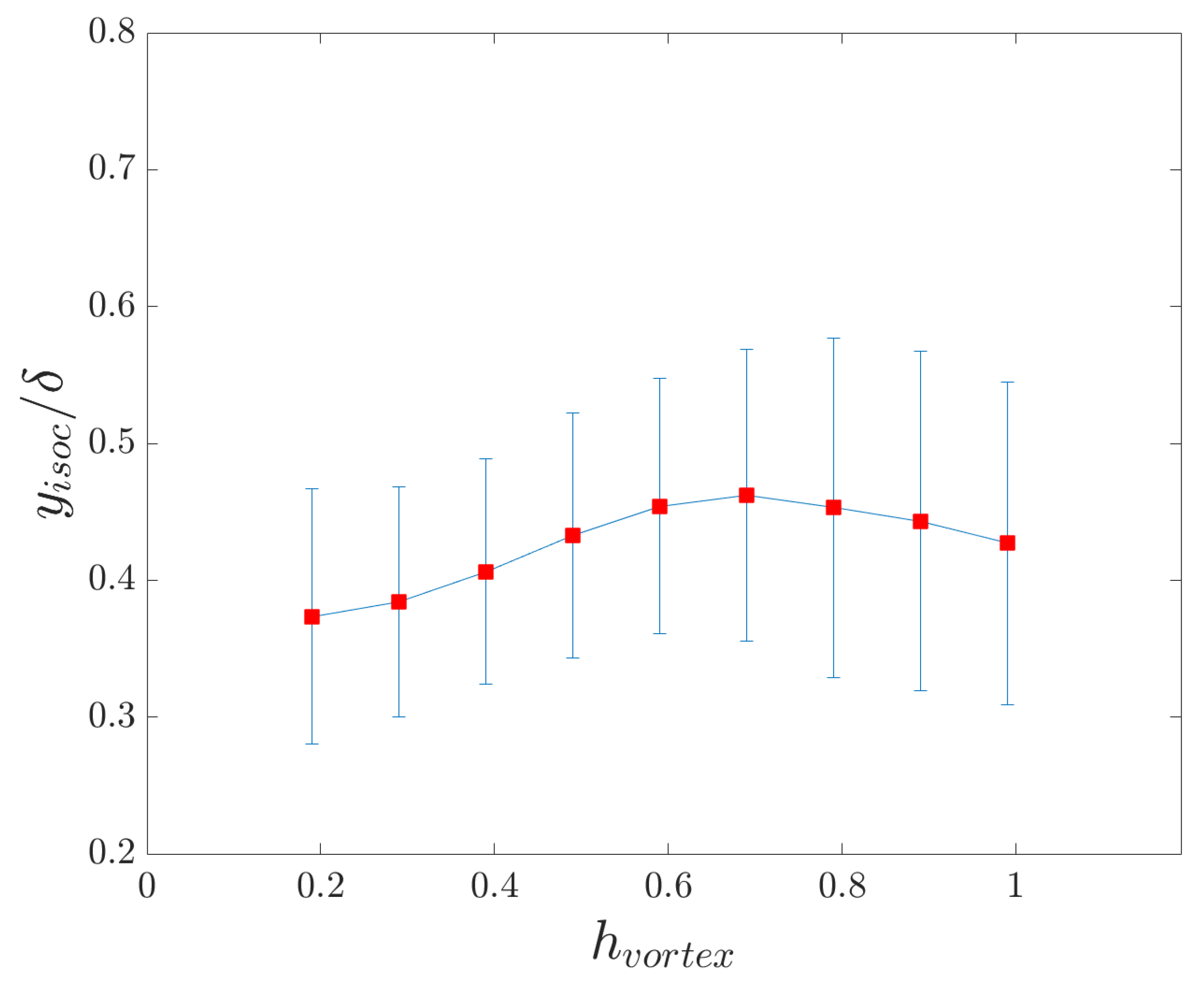
As an alternative comparison between the large-scale streamwise velocity field and the height of coherent vortices in the flow, the height of an isocontour of the complete or non-fluctuating large-scale streamwise velocity field, , was compared to the local height of the vortices. Using the same binning methodology as described before, the average height of the isocontour was plotted alongside the standard deviation for each bin, as shown in Figure 7. The blue lines indicate the standard deviation for each bin while the red squares denote the mean height of large-scale velocity isocontour for each bin. The mean height of the chosen isocontour is found to increase as the height of the vortex increases.
4. Discussion
The location of coherent vortex structures was shown to be correlated to the local behavior of large-scale velocity structures. Conditionally averaging on the height of coherent vortex structures identified fast large-scale streamwise velocity structures above vortex structures that were nearer to the wall (Figure 4a) and slow large-scale streamwise velocity structures below vortex structures that were farther from the wall (Figure 4b). Large-scale streamwise velocity profiles are shown in Figure 5 to demonstrate near-wall positive velocity signatures for wake region vortices nearer to the wall and negative velocity far from the wall for wake region vortices farther from the wall. A new correlation coefficient was defined between a fluctuating vortex height and the fluctuating large-scale streamwise velocity signal and was found to be largely negative, with large negative values in the upper 40% of the boundary layer. The height of a local large-scale streamwise isocontour was identified and conditioned based on the height of a vortex, and was observed to vary from nearer to the wall for nearer vortices to farther from the wall for farther vortices.
Each identified vortex has a small-scale velocity signature, as highlighted in Figure 2. Previous studies identified relationships between the envelope or intensity of small-scale velocity and the large-scale velocity [26,28,29] and found that large-scale velocity amplitude is correlated to the envelope and intensity of small-scale velocity, with a dependency that is a function of wall-normal location. Far from the wall, low-speed streamwise large-scale velocity is associated with a larger envelope and intensity of small-scale velocity, while near the wall, high-speed streamwise large-scale velocity is associated with a larger envelope and intensity of small-scale velocity. The present work’s focus on coherent vortices can be seen as a study of a subset of the signatures studied by the works of Mathis et al. [26] and Chung and McKeon [29]. Rather than study all of the small-scale signals, the present work studies the strongest coherent signals, identified using vorticity but that also have a strong and coherent small-scale velocity signal, and identifies relationships between the location where the strongest signals occur and the local amplitude of large-scale velocity. If the pattern observed was inconsistent with the results of amplitude modulation [26] and conditional averaging [29] between large- and small-scale velocity signals, it would indicate that vortex organisation is distinct from the observations made by these researchers, and that the phenomena they study corresponds to a different physical mechanism. If the pattern observed for the vortices was consistent with the results between large- and small-scale velocity signals, it might indicate that vortex organisation was part of the organisation that was identified using amplitude modulation and conditional averaging.
The present findings indicate that vortices are stronger above regions of large-scale, low-speed streamwise velocity and stronger below regions of large-scale, high-speed streamwise velocity within the wake region of the boundary layer. The identification of strong vortices within and above regions of large-scale, low-speed streamwise velocity is consistent with the attached eddy model [6], the hairpin vortex hypothesis [2,7], and vortex cluster organisation [8]. The existence of strong vorticity and also small-scale velocity signals far from the wall in the presence of large-scale, low-speed streamwise velocity and nearer to the wall in the presence of large-scale, high-speed streamwise velocity is consistent with the conditional averaging results of Chung and McKeon [29]. Chung and McKeon [29] observed a variation in the height where small-scale intensity was strongest within a given region of the flow depending on the local sign of the large-scale velocity field. They also observed a symmetry in that property: large-scale, low-momentum regions correlated to the presence of small-scale intensity far from the wall, as suggested by the hairpin packet perspective, and large-scale, high-momentum regions correlated to the presence of small-scale intensity nearer to the wall, which was not a central property of the hairpin packet perspective.
The vortices’ proximity to specific isocontours of the large-scale streamwise velocity, shown in Figure 7, is also consistent with the shear layer results of de Silva et al. [20] and Heisel et al. [18]. Shear layers tend to lie upstream and above low-momentum regions and downstream and below high-momentum regions [20], which is again consistent with the structural observations of this work and others.
The focus on coherent vortex structures in this work may serve to usefully unite some of the findings of Adrian et al. [7] and Heisel et al. [17], concerning vortex organisation, with those of Mathis et al. [26] and Chung and McKeon [29].
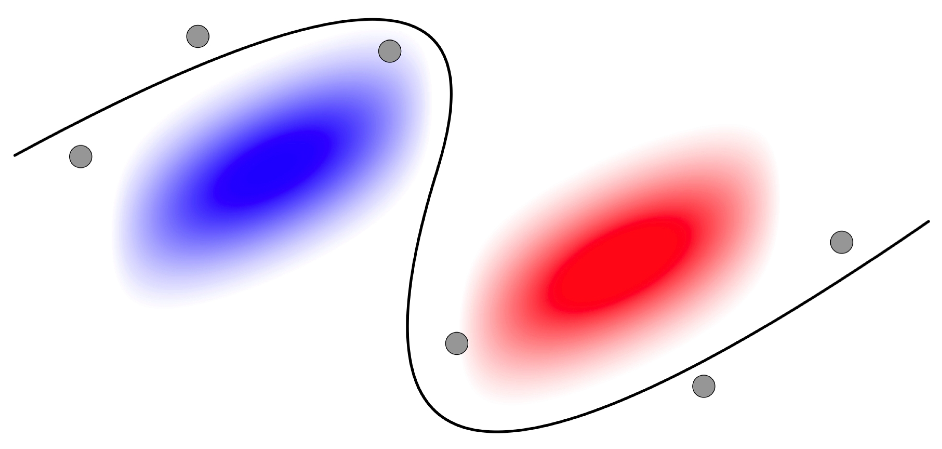
Figure 8 illustrates the findings of this study in the form of a model schematic. The red and blue ellipses in the figure denote high and low-speed large-scale events in the flow while the black solid line indicates the full large-scale streamwise velocity isocontour. The smaller grey coloured circles indicate the position of coherent vortices in the boundary layer. As discussed, our results suggest that when the local large-scale velocity is negative, the vortices tend to be farther away from the wall, while when the local large-scale velocity is positive, the vortices tend to be nearer to the wall, which is shown in the schematic. The isocontour is algebraically related to the fluctuating signals, rising in the presence of a large-scale negative streamwise velocity structure, and falling in the presence of a large-scale positive streamwise velocity structure [30].
Future efforts will be directed towards quantifying the spacing and size of the coherent vortices at their variable heights in the flow, as well as the dependence of these observations on Reynolds number. Vortex spacing will be quantified at particular heights in the flow and along curved isocontours of the large-scale streamwise velocity field.
Author Contributions
Conceptualization, S.S. and T.S.-F.; methodology, S.S. and T.S.-F.; software, S.S.; validation, S.S.; formal analysis, S.S.; investigation, T.S.-F. and S.S.; resources, T.S.-F.; data curation, T.S.-F.; writing—original draft preparation, S.S.; writing—review and editing, S.S. and T.S.-F.; visualization, S.S.; supervision, T.S.-F.; project administration, T.S.-F.; funding acquisition, T.S.-F. Both authors have read and agreed to the published version of the manuscript.
Funding
The authors would like to thank the Grainger College of Engineering and the Aerospace Engineering department of the University of Illinois at Urbana-Champaign for their support of this research.
Data Availability Statement
Data supporting these results can be acquired through direct inquiry to the last author, Theresa Saxton-Fox, at [email protected].
Acknowledgments
The authors would like to thank Elizabeth Torres-De Jesus for productive discussions and constructive feedback on the paper.
Conflicts of Interest
The authors declare no conflict of interest. The funders had no role in the design of the study; in the collection, analyses, or interpretation of data; in the writing of the manuscript, or in the decision to publish the results.
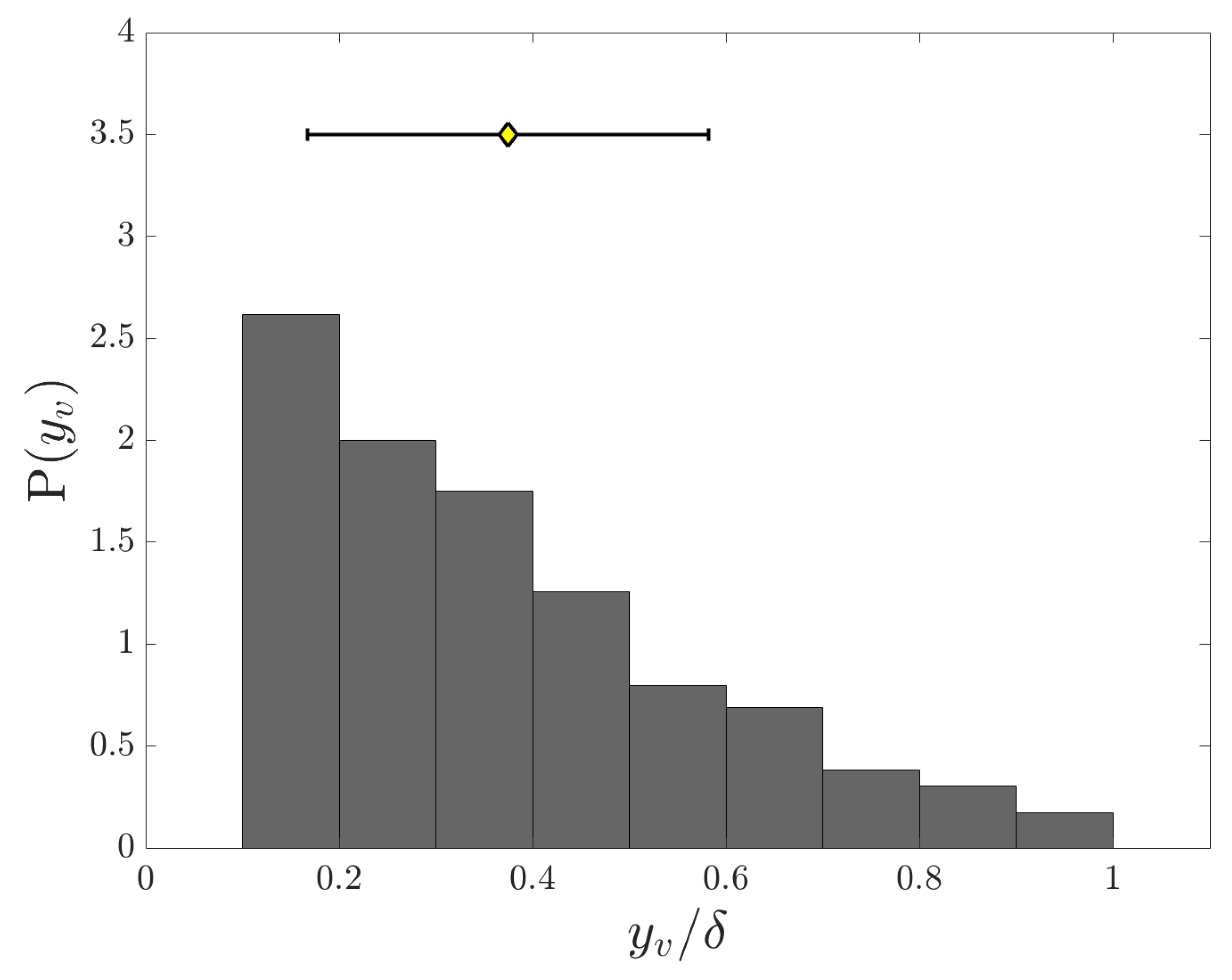
Appendix A. Probability Density Function of the Vortex Heights y v
The height of all detected vortices was skewed towards nearer the wall, which agrees with the attached eddy model of Perry and Chong [6]. Figure A1 shows the probability density function of the vortex heights with the mean and standard deviation. The figure indicates a gradual decrease in the number of vortices as the height of the vortices increases.
Figure A1.
Probability Density Function P() of the height of the vortices. The yellow diamond marker indicates the mean height of all vortices and the error-bar shows the standard deviation in the data.
Figure A1.
Probability Density Function P() of the height of the vortices. The yellow diamond marker indicates the mean height of all vortices and the error-bar shows the standard deviation in the data.

References
- Robinson, S.K. Coherent motions in the turbulent boundary layer. Annu. Rev. Fluid Mech. 1991, 23, 601–639. [Google Scholar] [CrossRef]
- Adrian, R.J. Hairpin vortex organization in wall turbulence. Phys. Fluids 2007, 19, 041301. [Google Scholar] [CrossRef] [Green Version]
- Theodorsen, T. Mechanism of turbulence. In Proceedings of the Mid-Western Conference on Fluid Mechanics, Columbus, OH, USA, 17–19 March 1952. [Google Scholar]
- Head, M.R.; Bandyopadhyay, P.R. New aspects of turbulent boundary-layer structure. J. Fluid Mech. 1981, 107, 297–338. [Google Scholar] [CrossRef]
- Falco, R.E. Coherent motions in the outer region of turbulent boundary layers. Phys. Fluids 1977, 20, S124–S132. [Google Scholar] [CrossRef]
- Perry, A.E.; Chong, M.S. On the mechanism of wall turbulence. J. Fluid Mech. 1982, 119, 173–217. [Google Scholar] [CrossRef] [Green Version]
- Adrian, R.J.; Meinhart, C.D.; Tomkins, C.D. Vortex organization in the outer region of the turbulent boundary layer. J. Fluid Mech. 2000, 422, 1–54. [Google Scholar] [CrossRef] [Green Version]
- Lozano-Durán, A.; Flores, O.; Jiménez, J. The three-dimensional structure of momentum transfer in turbulent channels. J. Fluid Mech. 2012, 694, 100–130. [Google Scholar] [CrossRef]
- De Silva, C.M.; Hutchins, N.; Marusic, I. Uniform momentum zones in turbulent boundary layers. J. Fluid Mech. 2016, 786, 309–331. [Google Scholar] [CrossRef] [Green Version]
- Eich, F.; de Silva, C.M.; Marusic, I.; Kähler, C.J. Towards an improved spatial representation of a boundary layer from the attached eddy model. Phys. Rev. Fluids 2020, 5, 034601. [Google Scholar] [CrossRef]
- Deshpande, R.; de Silva, C.M.; Lee, M.; Monty, J.P.; Marusic, I. Data-driven enhancement of coherent structure-based models for predicting instantaneous wall turbulence. arXiv 2021, arXiv:2107.01750. [Google Scholar]
- Kim, J.; Moin, P.; Moser, R.D. Turbulence statistics in fully developed channel flow at low Reynolds number. J. Fluid Mech. 1987, 177, 133–166. [Google Scholar] [CrossRef] [Green Version]
- Jiménez, J.; Hoyas, S.; Simens, M.P.; Mizuno, Y. Turbulent boundary layers and channels at moderate Reynolds numbers. J. Fluid Mech. 2010, 657, 335–360. [Google Scholar] [CrossRef] [Green Version]
- Eitel-Amor, G.; Örlü, R.; Schlatter, P.; Flores, O. Hairpin vortices in turbulent boundary layers. Phys. Fluids 2015, 27, 025108. [Google Scholar] [CrossRef]
- Motoori, Y.; Goto, S. Hairpin vortices in the largest scale of turbulent boundary layers. Int. J. Heat Fluid Flow 2020, 86, 108658. [Google Scholar] [CrossRef]
- Rao, K.N.; Narasimha, R.; Narayanan, M.A.B. The ‘bursting’ phenomenon in a turbulent boundary layer. J. Fluid Mech. 1971, 48, 339–352. [Google Scholar] [CrossRef] [Green Version]
- Heisel, M.; Dasari, T.; Liu, Y.; Hong, J.; Coletti, F.; Guala, M. The spatial structure of the logarithmic region in very-high-Reynolds-number rough wall turbulent boundary layers. J. Fluid Mech. 2018, 857, 704–747. [Google Scholar] [CrossRef]
- Heisel, M.; de Silva, C.M.; Hutchins, N.; Marusic, I.; Guala, M. Prograde vortices, internal shear layers and the Taylor microscale in high-Reynolds-number turbulent boundary layers. J. Fluid Mech. 2021, 920, A52. [Google Scholar] [CrossRef]
- Bautista, J.C.C.; Ebadi, A.; White, C.M.; Chini, G.P.; Klewicki, J.C. A uniform momentum zone–vortical fissure model of the turbulent boundary layer. J. Fluid Mech. 2019, 858, 609–633. [Google Scholar] [CrossRef]
- De Silva, C.M.; Philip, J.; Hutchins, N.; Marusic, I. Interfaces of uniform momentum zones in turbulent boundary layers. J. Fluid Mech. 2017, 820, 451–478. [Google Scholar] [CrossRef] [Green Version]
- Monty, J.P.; Hutchins, N.; Ng, H.C.H.; Marusic, I.; Chong, M.S. A comparison of turbulent pipe, channel and boundary layer flows. J. Fluid Mech. 2009, 632, 431–442. [Google Scholar] [CrossRef]
- Kim, K.C.; Adrian, R.J. Very large-scale motion in the outer layer. Phys. Fluids 1999, 11, 417–422. [Google Scholar] [CrossRef]
- Kline, S.J.; Reynolds, W.C.; Schraub, F.A.; Runstadler, P.W. The structure of turbulent boundary layers. J. Fluid Mech. 1967, 30, 741–773. [Google Scholar] [CrossRef] [Green Version]
- Blackwelder, R.F.; Eckelmann, H. On the wall structure of the turbulent boundary layer. J. Fluid Mech. 1967, 76, 89–112. [Google Scholar] [CrossRef]
- Jiménez, J.; Pinelli, A. The autonomous cycle of near-wall turbulence. J. Fluid Mech. 1999, 389, 335–359. [Google Scholar] [CrossRef] [Green Version]
- Mathis, R.; Hutchins, N.; Marusic, I. Large-scale amplitude modulation of the small-scale structures in turbulent boundary layers. J. Fluid Mech. 2009, 628, 311–337. [Google Scholar] [CrossRef] [Green Version]
- Bernardini, M.; Pirozzoli, S. Inner/outer layer interactions in turbulent boundary layers: A refined measure for the large-scale amplitude modulation mechanism. Phys. Fluids 2011, 23, 061701. [Google Scholar] [CrossRef]
- Baars, W.; Hutchins, N.; Marusic, I. Reynolds number trend of hierarchies and scale interactions in turbulent boundary layers. Philos. Trans. R. Soc. A Math. Phys. Eng. Sci. 2017, 375, 20160077. [Google Scholar] [CrossRef] [PubMed]
- Chung, D.; McKeon, B.J. Large-eddy simulation of large-scale structures in long channel flow. J. Fluid Mech. 2010, 661, 341–364. [Google Scholar] [CrossRef] [Green Version]
- Saxton-Fox, T.; McKeon, B.J. Coherent structures, uniform momentum zones and the streamwise energy spectrum in wall-bounded turbulent flows. J. Fluid Mech. 2017, 826, R6. [Google Scholar] [CrossRef]
- Kolář, V. Vortex identification: New requirements and limitations. Int. J. Heat Fluid Flow 2007, 28, 638–652. [Google Scholar] [CrossRef]
Figure 1.
A contour plot of , highlighting regions of coherent rotation in the flow. The black ellipse indicates a strong peak in , corresponding to the locally strongest spanwise vortex. The solid vertical lines indicate the streamwise width of the region of vortex identification while the dotted vertical lines indicate the sampling window for the large-scale velocity field. The sampling window is differently placed for each snapshot and is always decided such that the identified vortex is in the center in the streamwise direction while the region of vortex identification is same for all snapshots.

Figure 2.
The velocity vector field in a frame-of-reference convecting at . The rectangle highlights the identified vortex in the flow.
Figure 2.
The velocity vector field in a frame-of-reference convecting at . The rectangle highlights the identified vortex in the flow.

Figure 3.
Magnitude of the fluctuating small-scale velocity field . The black ellipse shows the position of the detected vortex in the flow
Figure 3.
Magnitude of the fluctuating small-scale velocity field . The black ellipse shows the position of the detected vortex in the flow

Figure 4.
Conditionally averaged fluctuating large-scale velocity fields based on the height of small-scale vortices. (a) shows the conditionally averaged fluctuating large-scale velocity field for while (b) shows the conditionally averaged fluctuating large-scale velocity field for . The yellow triangle indicates the mean position of the small-scale vortices while the error-bar shows the standard deviation in the heights of the vortices identified.

Figure 5.
Average fluctuating streamwise large-scale velocity profiles plotted against wall-normal height. Four different ranges of heights of the coherent vortices were used to group the streamwise large-scale velocity data: shown in blue, shown in red, shown in yellow, and shown in purple.
Figure 5.
Average fluctuating streamwise large-scale velocity profiles plotted against wall-normal height. Four different ranges of heights of the coherent vortices were used to group the streamwise large-scale velocity data: shown in blue, shown in red, shown in yellow, and shown in purple.

Figure 6.
A plot of correlation coefficient, R, against normalised height of the vortex . The red squares indicate the mean correlation at each binned height.
Figure 6.
A plot of correlation coefficient, R, against normalised height of the vortex . The red squares indicate the mean correlation at each binned height.

Figure 7.
The height of the large-scale streamwise velocity isocontour at against height of the coherent vortices. The red squares indicate the mean height of the isocontour for a given while the blue lines indicate the standard deviation of the isocontour height.
Figure 7.
The height of the large-scale streamwise velocity isocontour at against height of the coherent vortices. The red squares indicate the mean height of the isocontour for a given while the blue lines indicate the standard deviation of the isocontour height.

Figure 8.
A schematic showing the preferential arrangement of coherent vortices along large-scale velocity isocontours and their relationship to large scale structures. The red and blue ellipse here denote high and low-speed large-scale structures respectively while the black solid line denotes a velocity iso-contour. The smaller grey circles indicate the position of coherent vortices in the flow.

Publisher’s Note: MDPI stays neutral with regard to jurisdictional claims in published maps and institutional affiliations. |
© 2021 by the authors. Licensee MDPI, Basel, Switzerland. This article is an open access article distributed under the terms and conditions of the Creative Commons Attribution (CC BY) license (https://creativecommons.org/licenses/by/4.0/).
Share and Cite
MDPI and ACS Style
Shrivastava, S.; Saxton-Fox, T. Correlation between Large-Scale Streamwise Velocity Features and the Height of Coherent Vortices in a Turbulent Boundary Layer. Fluids 2021, 6, 286. https://0-doi-org.brum.beds.ac.uk/10.3390/fluids6080286
AMA Style
Shrivastava S, Saxton-Fox T. Correlation between Large-Scale Streamwise Velocity Features and the Height of Coherent Vortices in a Turbulent Boundary Layer. Fluids. 2021; 6(8):286. https://0-doi-org.brum.beds.ac.uk/10.3390/fluids6080286
Chicago/Turabian StyleShrivastava, Shaurya, and Theresa Saxton-Fox. 2021. "Correlation between Large-Scale Streamwise Velocity Features and the Height of Coherent Vortices in a Turbulent Boundary Layer" Fluids 6, no. 8: 286. https://0-doi-org.brum.beds.ac.uk/10.3390/fluids6080286