1. Introduction
Accurate modeling of compressible turbulent flows required in aerospace industry, including aeronautical and rotorcraft engineering, turbomachinery, automotive and railway transportation, energy and several technology-related industries, continues to be one of the major challenges in developing simulation-based predictive tools that can be used for design and analysis of fluid engineering systems and/or their components [
1]. Compared to the low-Mach number incompressible regime, the computational fluid dynamics of high-speed compressible flows is further complicated by significant variations of the fluid thermodynamic properties. The highest fidelity method, i.e., direct numerical simulation (DNS) remains computationally prohibitive for moderate to high Reynolds-number flows, due to the need to resolve an extremely wide range of length and time scales that results in computational requirements exceeding current capabilities. The number of grid points (degrees of freedom) required for DNS is proportional to either
, based on the large eddy characteristic velocity and length scales [
2], or
, based on the stream-wise domain size [
3]. Due to the high accuracy requirements for the spatial discretization, spectral methods [
4] and compact finite difference methods [
5] are the most popular numerical schemes for DNS. However, their applications to complex geometries in realistic engineering problems are still limited. Therefore, more efficient numerical methods than DNS are of great interest in simulations of large scale complex flows.
In order to increase the computational efficiency of turbulent flow simulations and substantially improve the accuracy of predictions of fluid flow characteristics, a number of wavelet-based adaptive numerical methodologies [
6,
7,
8] that explore unique properties of wavelet analysis to unambiguously identify and isolate localized flow structures have been developed. These methods allow to fully utilize spatial/temporal turbulent flow intermittency and to tightly integrate numerics and physics-based turbulence modeling [
9,
10,
11,
12], while resolving dynamically dominant flow structures with an active error control and ensuring better capture of the flow physics on a nearly optimal adaptive computational grid, ultimately leading to substantial reduction in the computational cost. Specifically, for the results reported in Refs. [
12,
13,
14,
15,
16,
17], the reduction of grid points number results in being above 90% for most of three-dimensional (3D) cases, compared to the full mesh at the highest level of resolution.
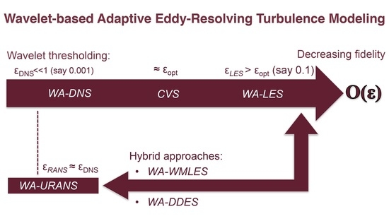
Furthermore, tight integration of wavelet-based adaptive numerical methods with turbulence modeling allows to construct a hierarchical eddy-capturing framework for simulating compressible turbulent flows, where coherent flow structures are either totally or partially resolved on self-adaptive computational grids, while modeling the effect of unresolved motions, wherever it is appropriate. The separation between resolved (more energetic, coherent) eddies and residual (less energetic, coherent/incoherent) flow structures is achieved by means of the nonlinear wavelet thresholding filter (WTF). The value of wavelet threshold controls the relative importance of resolved field and residual background flow and, thus, the fidelity of turbulence simulations. By increasing the thresholding level, a unified hierarchy of wavelet-based eddy-capturing turbulence models of progressively lower fidelity is obtained, namely, the wavelet-based adaptive direct numerical simulation (WA-DNS) [
12], the coherent vortex simulation (CVS) [
18], and the wavelet-based adaptive large eddy simulation (WA-LES) [
11,
19,
20,
21].
A distinct advantage of this adaptive eddy-capturing framework is that the overall physical fidelity of the simulation can be simply controlled by the WTF strength [
22,
23], thereby providing a hierarchical modeling framework that allows continuous transition among the various fidelity regimes. In fact, transition from WA-DNS to CVS, and to WA-LES, is well established through controlling the wavelet threshold. WA-DNS uses wavelet-based discretization of the (unfiltered) Navier–Stokes equations to dynamically adapt the local resolution on intermittent flow structures [
24,
25]. Transition from WA-DNS to CVS is achieved by using an optimal wavelet threshold [
18], resulting in the decomposition of the flow field into coherent and incoherent contributions. For WA-LES, the wavelet threshold is further increased so that the stochastic and the least energetic coherent portion of the turbulent solution are discarded, and only the most energetic part of the coherent vortices are captured in the resolved field [
19]. In WA-LES, the discarded subgrid-scale (SGS) coherent structures dominate the total SGS dissipation to be modeled [
26,
27]. Therefore, similar to conventional non-adaptive LES, deterministic closures [
28,
29] are applicable for WA-LES by modeling SGS coherent structures in terms of resolved energetic coherent vortices. A recent comprehensive review about the hierarchical adaptive eddy-capturing approach for modeling incompressible turbulent flows can be found in Ref. [
30].
As far as the simulation of wall-bounded high Reynolds-number flows is concerned, the reliable and computationally efficient prediction of the effects of near-wall turbulence still represents the major challenge for the turbulence modeling community. Recently, a number of wall-modeled and wall-resolved wavelet-based adaptive approaches have been developed [
14,
16,
31,
32]. Several attempts for the application of the wavelet-based methods have been carried out for both wall-modeled and wall-resolved simulations. In the latter case, the wall region is fully resolved by the wavelet-based adaptive computational mesh and no wall model is needed. Thus, the wall-resolved WA-LES [
14] can be directly applied. However, even with wavelet-based grid adaptation, the computational cost of wall-resolved simulations at high Reynolds numbers is prohibitively high. Thus, the Reynolds-averaged Navier–Stokes (RANS) modeling approach is still of great importance in engineering applications. The capabilities of the recently developed wavelet-based adaptive unsteady RANS (WA-URANS) method [
16,
31,
32] have been demonstrated for a variety of two-dimensional (2D) and three-dimensional (3D) high Reynolds-number complex geometry flows, for different speed regimes and various boundary conditions.
Although the RANS methods are very popular in a wide range of industrial applications, more accurate simulations become more and more demanding in some areas, especially considering the fast development of high performance computing [
1]. To compromise the accuracy and efficiency between the wall-resolved LES and RANS approaches, the wall-modeled LES has drawn great attention in the last two decades. In fact, as estimated by Choi and Moin [
3], the computational complexity of the wall-resolved LES approach scales as ∼
, whereas for the wall-modeled LES [
33,
34] it scales as ∼
. Therefore, the latter approach is more applicable to high Reynolds number problems, despite some side-effects, such as the log-layer mismatch (LLM). Due to LLM, where near-wall RANS and resolved LES away from the wall do not quite match their interception constants in the log-law layers, the error in skin friction of about 5% to 15% is observed [
35,
36,
37].
There are three well-known categories of wall-modeled LES methods: (1) the hybrid LES/RANS methods [
38,
39,
40,
41], (2) the Detached-Eddy Simulation (DES) methods [
35,
36,
42,
43] and (3) the wall-shear-stress modeled methods [
44,
45,
46,
47,
48]. Both the first two categories switch to RANS formulation in the inner layer of the wall region. The hybrid LES/RANS methods usually use a RANS closure model in the near-wall region and an LES approach away from the wall. In this category, the terms zonal and nonzonal are used to identify different methods. For zonal methods, a RANS zone is specified in advance, whereas nonzonal methods usually use a blending function to interpolate between RANS and SGS turbulent stresses. Note that in the DES community, DES methods are usually also referred to as hybrid LES/RANS methods. However, the DES approach appears to have a more “seamless” inter-model transition based on length scale that switches to either a RANS formulation or the general LES closure model, and can be considered as a unified closure model throughout the domain [
49]. Finally, the wall-shear-stress methods model the wall shear stress directly on the wall by performing a RANS computation on a separate boundary layer mesh and returning wall stress and heat flux as boundary conditions for the large eddy simulation.
To build a framework for the application of wall-modeled LES approaches in the wavelet-based adaptive methodology, the first question to address is how the WA-LES and WA-URANS can coexist in a single simulation. The transition from WA-LES to WA-URANS is not as straightforward as the aforementioned transition from WA-DNS to CVS, and to wall-resolved WA-LES. In the compressible RANS modeling framework, the unknown variables represent mean (Reynolds- or Favre-averaged) quantities, which are smooth and whose evolution is simulated by modeling the mean effects of turbulent stresses. In fact, as shown in Refs. [
16,
32], the accurate solution of the WA-URANS equations requires wavelet threshold values as small as the ones used in WA-DNS. This is counterintuitive when looking at the increasing fidelity regime for monotonically decreasing WTF level, as previously discussed. However, although a low level of wavelet threshold is used to achieve high numerical accuracy, the smooth mean solution of the governing equations turns out to be supported by a relatively coarse adaptive mesh, regardless how fine the mesh at the highest permitted level of resolution is.
To develop a hybrid, mathematically consistent approach with coexistence and connection between WA-URANS and WA-LES approaches, the wavelet-based adaptive delayed detached eddy simulation (WA-DDES) formulation was recently proposed [
15,
50]. A variable wavelet thresholding strategy was used to blend a very small wavelet threshold in the WA-URANS region with a relatively large value in the WA-LES region. The developed wavelet-based adaptive extension allows to achieve both accuracy and efficiency in terms of degrees of freedom used in WA-DDES compared to the wall-resolved WA-LES. However, the stringent restriction on the time integration step caused by the CFL-type [
51] condition still remains to be a major issue for WA-DDES computations. In fact, despite the use of highly stretched meshes with relatively large spacings in the wall-parallel directions to reduce the total number of active nodes, a relatively small wall-normal mesh spacings are employed in the region immediately adjacent to the wall, i.e., where
. To overcome this restriction, the new wavelet-based adaptive wall-modeled LES (WA-WMLES) method has been introduced in Ref. [
17], where the outer-layer WA-LES is supplied with a compressible equilibrium wall-stress model, so that the first mesh point away from the wall may be located at
, thus, relieving the time step restriction.
The development of WA-URANS, WA-DDES, and WA-WMLES, as well as (wall-resolved) WA-LES practically covers the full spectrum of wall-bounded turbulence modeling approaches. Along with WA-DNS and CVS, these methods serve as segregated steps towards the construction of a unified wavelet-based adaptive hierarchical eddy-resolving framework for modeling complex wall-bounded compressible turbulent flows, capable of performing simulations with various fidelity, from no-modeling DNS to full-modeling RANS, depending on the requirement and balance of accuracy and computational efficiency.
In the hierarchical adaptive
eddy-capturing approach [
30] the form of governing equations is kept unchanged and the transition between models of different fidelity is achieved through modifying the WTF level. The adaptive
eddy-resolving framework, discussed in this review, incorporates a wider class of methods that not only utilize different wavelet thresholds but also include different governing equations with
model-form adaptation. In particular, the combination of these two features facilitates the development of wavelet-based adaptive wall-modeled approaches. The present work represents the original attempt at systematically expanding the application of the wavelet-based adaptive methodology for accurate and efficient predictions of complex wall-bounded turbulent flows.
The rest of the paper is organized as follows.
Section 2 introduces the wavelet-based Favre filtered/averaged Navier–Stokes equations. In
Section 3, the wavelet-based method that is used for the numerical implementations is described.
Section 4 and
Section 5 describe wall-resolved and wall-modeled methods, respectively, with discussion of key concepts, advantages/disadvantages of each method, as well as simulation examples. Finally, some concluding remarks are given in
Section 6.
2. Wavelet-Favre Filtered/Averaged Navier–Stokes Equations
In this section, the wavelet-based Favre filtered/averaged Navier–Stokes equations for compressible turbulent flows are presented. For simplicity, Favre filtered equations for LES computations and Favre averaged equations for RANS computations are combined into a common form, with explanation of meanings of the integrated variables and modeled terms for the two distinguished formulations.
WA-LES is formulated in terms of wavelet-based spatially filtered variables. For conventional non-adaptive LES, the implicit or explicit linear lowpass filtering operator is usually defined a priori and is tied to the corresponding computational mesh, with under-resolved mesh spacings relative to DNS. In contrast to standard LES, the spatial filter used in WA-LES is constructed by employing the WTF operator described in
Section 3, which is nonlinear and depends on the instantaneous flow realization. In the following, the WTF operator is denoted by
, where
stands for the prescribed level of thresholding. Similarly to the conventional lowpass-Favre filter for variable density flows, the wavelet-Favre filter is defined by
. This way, the wavelet-Favre filtered Navier–Stokes equations involve the following primitive variables:
,
,
,
and
, representing, respectively, wavelet-filtered density and pressure, together with wavelet-Favre filtered velocity, temperature and total energy (per unit mass).
Differently, WA-URANS is formulated in terms of Reynolds-averaged and Favre-averaged dependent variables. Denoting Reynolds-averaging and Favre-averaging operations as and , respectively, where stands for a generic physical variable, the method involves and , together with , , and . Note that, in this context, since a very low level of wavelet thresholding is used, the effect of WTF is practically negligible, and the corresponding operator symbol is omitted in the notations of Reynolds/Favre-averaged primitive variables.
Furthermore, WA-DDES is formulated in terms of both Reynolds-averaged and spatially (wavelet) filtered quantities, which exist simultaneously in this hybrid modeling framework. In fact, the family of eddy-resolving DES models is better described in terms of length scale formulations [
49], where either Reynolds-averaged in the near-wall region (referred to as RANS region) or low-pass wavelet-filtered Navier–Stokes equations away from the wall (LES region) are solved. DES results in being, essentially, an eddy-resolving method everywhere as it has to be ensemble-averaged to obtain meaningful statistical quantities. Significant levels of fluctuations are usually observed, even in the RANS regions of the flow domain. Therefore, in WA-DDES, all dependent variables can be interpreted as Favre-filtered quantities.
For the sake of clarity, the simple symbols
,
p,
,
T and
e are used hereafter to denote the resolved primitive variables for either WA-LES or WA-URANS formulations, including WA-WMLES and WA-DDES. Therefore, the wavelet-Favre filtered/averaged Navier–Stokes equations governing the balance of mass, momentum, and energy in compressible flows of a calorically perfect gas, supplied with modeled turbulent terms, can be written in the following general form:
where
The parameter R stands for the gas constant, while and are the specific heats at constant pressure and volume, respectively, where the specific heat ratio for diatomic gases is assumed. The term represents the sum of molecular and modeled turbulent heat fluxes, with being the Prandtl number, where is the thermal conductivity, and the turbulent Prandtl number. In this work, these two parameters are assumed constant, being set to and , respectively. Note that the temperature dependent molecular dynamic viscosity is given by the Sutherland’s law. The turbulent eddy viscosity is denoted by , which is unknown and needs a turbulence model for closure. The term is the sum of molecular and modeled stress tensors, while is the mean strain-rate tensor, with representing the associated deviatoric part, is the Kronecker delta, and the summation convention for repeated indices is assumed.
The definition of the stress tensor depends on the formulation that is applied. In WA-LES, where the wavelet-Favre filtered equations are considered, the SGS stress tensor is defined as
where the unclosed term
involves the unfiltered velocity
. In WA-URANS, where the Favre averaged equations are considered, the Reynolds stress tensor is written as
where the unclosed term
involves the instantaneous velocity
. Regardless of the formulation, the residual stress tensor is modeled according to the eddy-viscosity assumption, namely,
so that
holds for the total stress tensor (7). All the details about the governing equations and turbulence closure models can be found in the reference articles for the different approaches that are WA-LES [
14], WA-URANS [
16], WA-DDES [
15], and WA-WMLES [
17].
3. Adaptive Wavelet Collocation Method
Regardless of the adopted formulation, the governing equations described in the previous section are numerically solved using the parallel adaptive wavelet-collocation (AWC) method [
7]. This method is based on multi-resolution wavelet analysis to construct time-dependent computational meshes with spatially varying resolution that is required to adequately resolve the localized structures of the solution with a priori prescribed accuracy. From previous studies on different wavelet-based turbulence modeling methods for linearly forced homogeneous turbulence [
10] and supersonic channel flow [
15] the Reynolds number scaling of wavelet-based adaptive methods is considerably slower than cubic, i.e.,
, required for the non-adaptive DNS. However, further investigation on the
scaling of the models in wavelet-based eddy-resolving hierarchy at very high Reynolds numbers remains to be done, in order to apply the wavelet-based methods to practical industrial flows.
Formally, the mesh adaptation is based on the analysis of wavelet decomposition of a spatially dependent field, say
, sampled on a set of dyadic nested collocation points
at different levels of resolution
j, formally written as
where
n denotes the number of spatial dimensions, bold subscripts denote
n-dimensional indices, while
and
are
n-dimensional index sets associated with scaling functions
and different family wavelets
, respectively. Each of the basis functions, i.e.,
or
, has one-to-one correspondence with a mesh point
or
. Scaling functions
carry the averaged signal, while the multi-dimensional second-generation wavelet functions
define local, variational details. The amplitudes are given by the coefficients
and
, respectively, and hence have a unique correspondence to mesh points. The levels of resolution span over
, with 1 and
J being respectively the coarsest and finest levels of resolution present in the approximation. During the wavelet transform, detail (or wavelet) coefficients
are obtained recursively from scaling function coefficients
, from level
J to 2. After the wavelet transform, the coefficients
(
) and
(
) are stored, respectively, at the mesh points of the coarsest (
) and higher (
) levels of resolution. Note that for
n-dimensional space, there are (
) families of wavelet functions, which are indexed by
.
Wavelet-based filtering arises naturally from the series expansion (
12). The WTF operation is performed by applying the wavelet transform to the original field
, zeroing the wavelet coefficients below a given threshold, say
for generality, and transforming back to the physical space. The resulting approximate field, say
, composed of a subset of the original wavelets, represents the dominant modes and can be formally written as the following conditional series:
In many implementations, the filter threshold is taken to be relative to some characteristic scale, often represented by either the
or
norm of
taken globally over the domain and denoted as
[
19]. The resulting nonlinear filtering operation practically separates resolved flow structures and unresolved residual motions, where, for a properly normalized threshold, the reconstruction error of the filtered variable is shown to converge as
with
[
52].
The dynamic mesh adaptation is tightly coupled with WTF, because, due to the one-to-one correspondence between wavelets and grid points, the nodes are omitted from the computational mesh if the associated wavelets are excluded from the truncated approximation (
13). Indeed, the multilevel structure of the wavelet approximation provides a natural way to obtain the solution on a nearly optimal numerical mesh, which is dynamically adapted to the evolution of the main flow structures, both in location and scale, while higher resolution computations are carried out in the regions where (and only where) steep gradients in the resolved flow field occur. The multi-resolution wavelet decomposition (
13) is used for both mesh adaptation and interpolation, while the derivatives at the adaptive computational nodes are found by differentiation of the local wavelet interpolant at appropriate level of resolution [
6,
53].
It is worth noting that per-point cost of adaptive simulations is about three times more expensive for the AWC method with respect to corresponding non-adaptive simulations, which makes the adaptive method in principle outperform the corresponding non-adaptive one when less than one third of the mesh points are retained in the calculation or, equivalently, the grid compression ratio exceeds 67%. Based on the results reported in previous works [
12,
14,
15,
16,
17], typical compression ratios above 90% are observed for most 3D cases.
The second-generation wavelet bases described above rely on topologically rectilinear meshes and inherently isotropic mesh elements. This restriction puts some limitations on the applicability of the approach for simulation of complex geometry wall-bounded turbulent flows. These limitations were recently overcome with the development of the anisotropic AWC (A-AWC) method [
54]. This enhanced formulation preserves active error-controlling properties of the original method [
6,
7,
53,
55], but provides the additional flexibility to control mesh anisotropy and to solve flow problems in complex domains. In practice, by separating the computational space from the physical one and introducing a mapping between them, the use of anisotropic curvilinear meshes in complex geometries is permitted. At the same time, the structured rectilinear assembly of collocation points in the computational space is retained, which allows the use of computationally efficient discrete adaptive wavelet transform and derivative approximations. A-AWC utilizes a general curvilinear coordinate mapping function
, which can be either continuous or discrete. The mapping coordinates are viewed as additional variables, which can be adapted on and differentiated in computational space, thus, allowing the construction of the Jacobian matrix
Spatial derivatives in physical space are evaluated numerically as
where
is the inverse Jacobian matrix.
4. Wall-Resolving Approach
The WA-LES approach was extended for computational modeling of compressible wall-bounded attached turbulent flows in [
14], where the wavelet-Favre filtered compressible Navier–Stokes equations were derived. According to the wall-resolving approach, the spatial mesh was highly stretched in the wall-normal direction, with mesh spacings at the highest level of resolution practically corresponding to DNS-like resolution. Indeed, efficient and accurate calculations were permitted by the use of A-AWC method for the numerical implementation. The unknown SGS stresses (
9), together with the other unclosed terms in the governing equations, were approximated by means of eddy-viscosity/conductivity models based on the anisotropic minimum-dissipation (AMD) approach, which has low computational complexity while being particularly suitable for anisotropic grids [
56].
The performance of compressible WA-LES was assessed by conducting wall-resolved simulations of fully developed supersonic turbulent flow in a plane channel with isothermal cooled walls, at different Mach and Reynolds numbers [
14]. This flow configuration represents a well-established benchmark for wall-bounded turbulent compressible flows [
57]. In
Figure 1, an example of instantaneous adapted grid, colored by the thermal field normalized by the wall temperature, is reported for the flow case at
and
, which was simulated by prescribing
for WTF. As was expected, the spatial mesh resulted in being highly refined around localized flow structures. It is worth noting that the choice of the uniform level of thresholding is very important, especially when no explicit filtering operation is performed and the pure built-in filtering effect of AWC is exploited [
21]. This parameter was selected as a fair compromise to ensure the necessary numerical accuracy, while keeping acceptable the computational cost. The detailed discussion of how the WTF level affected the compressible WA-LES solution was also included in [
14].
Both feasibility and effectiveness of WA-LES in the high-speed compressible regime were demonstrated by making a comparison with reference DNS [
57] and LES [
58] of the same flow. The mesh resolution and some mean flow results for the three different solutions are presented in
Table 1, where the subscript
c is used to indicate values at the channel center. Note that, for WA-LES, while the resolution corresponding to an equivalent non-adaptive grid is shown for the two homogeneous directions, the minimum mesh spacing in the wall normal direction actually corresponds to the finest mesh that was employed in the simulation. The friction Reynolds and Mach numbers,
and
, as well as the heat flux coefficient,
, were reasonably predicted, consistently with non-adaptive LES data. Very importantly, the good agreement with reference DNS was obtained by retaining less than
of the AWC points at the highest level of resolution. As illustrated in
Figure 2, where the profiles of normalized mean density, temperature, and streamwise momentum are shown, WA-LES was able to almost perfectly reproduce mean flow features, which is fully consistent with reference LES data [
58]. Moreover, turbulent flow statistics were well predicted, as demonstrated by the profiles of turbulent shear stress and mean square temperature fluctuation depicted in
Figure 3. The accuracy of resolved turbulent fluctuations in the wall region demonstrated an important feature of compressible WA-LES. Close to the wall, owing to the automatic grid adaptation, the presence of high gradients in the mean flow-field variables, along with significant turbulent fluctuations, leaded to the use of refined grids. This fact must be taken into consideration when making a comparison between WA-LES and LES resolutions. Indeed, this behavior contributed to retain energy at high wavenumbers and caused the correspondingly increased local resolution with respect to conventional lowpass filter-based LES. In contrast, in the central region of the channel, due to the slowly spatially varying mean flow and less significant turbulence, coarser grids were employed in the calculation.


