

Aerodynamic Shape Optimization of a Symmetric Airfoil from Subsonic to Hypersonic Flight Regimes

1
IDMEC, Instituto Superior Técnico, Universidade de Lisboa, Av. Rovisco Pais, 1049-001 Lisboa, Portugal
2
Department of Mechanical Engineering, University of Victoria, Stn. CSC, Victoria, BC V8W 2Y2, Canada
*
Author to whom correspondence should be addressed.
Fluids 2022, 7(11), 353; https://0-doi-org.brum.beds.ac.uk/10.3390/fluids7110353
Submission received: 16 October 2022
/
Revised: 5 November 2022
/
Accepted: 8 November 2022
/
Published: 15 November 2022
(This article belongs to the Special Issue Recent Advances in Aerodynamics and Aeroacoustics: Towards Greener Aviation)
Abstract
:Hypersonic flight has been the subject of numerous research studies during the last eight decades. This work aims to optimize the aerodynamic performance of a two-dimensional baseline airfoil (NACA0012) at distinct flight regimes from subsonic to hypersonic speeds. A mission profile has been defined, where four points representing the subsonic, transonic, supersonic, and hypersonic flow conditions have been selected. A framework has been implemented based on high-fidelity RANS computational fluid dynamics simulations. Gradient-based optimizations have been conducted with the objective of minimizing the drag. The optimization results show an overall improvement in aerodynamic performance, including a decrease in the drag coefficient of up to 79.2% when compared to the baseline airfoil. In the end, a morphing strategy has been laid out based on the optimal shapes produced by the optimization.

1. Introduction
Air travel has become a common mode of transportation that is essential to connect cities and people, as well as to develop and reinforce economic ties. According to the International Civil Aviation Organization (ICAO) [1], in 2019, the number of passengers carried in scheduled services reached a record value of approximately 4.5 billion people. Hence, the demand for new and faster technologies has translated into an increasing attention to hypersonic transportation [2].
The study of hypersonic transport aircraft is motivated by the potential to fly further and faster, thus reducing travel times and pollutant emissions. Traveling from Brussels to Sydney in about three hours [3] or crossing the pacific ocean in less than two hours [4] are two potential outcomes enabled by hypersonic transportation. Moreover, the growing interest in space travel, such as space tourism or space exploration, also contributes to the interest in hypersonic flight.
To achieve hypersonic flight conditions, an aircraft must first experience subsonic, transonic, and supersonic speeds. Over such a wide speed range, the nature of the flow changes considerably. Consequently, the aircraft aerodynamic response will also vary. Therefore, the design of a hypersonic vehicle must take into account the balance of aerodynamic performances over its complete range of flight envelope [5]. The aerodynamic performance will lead to conflicting and even contradictory shape design requirements given the different flow physics involved [6].
Taking this a step further, it is desirable to optimize the aerodynamic performance of a vehicle in accordance with a set of flight conditions. Since the flight envelope is so wide, the significant variations in flow and aerodynamic performance will inevitably lead to conflicting shape-design requirements. Hence, an aerodynamic shape optimization (ASO) procedure is used to improve the aerodynamic performance by means of modifying its shape [7]. This procedure implies the use of parameterization techniques, which are used to accurately describe the body geometry.
However, designing an aircraft by means of ASO can represent a considerable computational effort, especially when a large amount of design variables is considered. The usage of the adjoint formulation [8] to compute the gradients allows for a computational cost reduction. Alternatively, surrogate models can also be employed, e.g., [9,10,11]. Even though the literature is vast in ASO applications for subsonic and transonic flows [7,12], for supersonic [13,14,15] and hypersonic [2,9,10,11,16] flows it is not as complete, especially in what concerns the latter one. Furthermore, the literature is even scarcer when several flow conditions are accounted for in the design process and to the best of the authors knowledge does not include hypersonic flow [13,17]. With this point in mind, the current work aims to provide a contribution to this topic by covering subsonic, transonic, supersonic, and hypersonic flows.
Finally, upon having the optimal design solutions for each flight condition, a morphing strategy can be studied and implemented, thus satisfying the multi-design and conflicting requirements. Morphing mechanisms are common in nowadays aviation, e.g., flaps and slats, improving the aerodynamic performance of aircraft at distinct flight segments [18,19]. This solution might enable one, in the future, to improve performance throughout different flow regimes, which are normally experienced by a hypersonic vehicle, if the complexity and weight of the required mechanism does not cancel the aerodynamic benefit.
The remainder of this article is organized as follows. The theoretical and mathematical background is presented in Section 2, followed by the methodology in Section 3, which describes the steps and procedures. In Section 4, the case study is formulated, and the results are presented in Section 5. Finally, conclusions are drawn in Section 6.
2. Background
The aerodynamic performance of a body moving through a fluid can be characterized by a given set of aerodynamic parameters of interest, such as the lift and drag coefficients, and , respectively. Moreover, the ratio between lift and drag forces also provides good insight into the aerodynamic response of the body. The accurate computation of these aerodynamic parameters depends on the correct description and modeling of the fluid behavior. By capturing the physical phenomena of interest, one is then capable of exploiting the aerodynamic data.
2.1. Governing Equations of Fluid Dynamics
The fluid behavior is described by a set of equations, which are derived from applying the principle of conservation laws to quantities such as the momentum, energy, or density. Commonly know as the Navier–Stokes equations, this set of conservative partial differential equations (PDE) is widely used in numerical simulations and experimental analyses.
Equation (1) presents the general form of the conservation equation, from which the Navier–Stokes equations are derived [20],
where represents the state variables vector, refers to the convective fluxes, and represents the viscous fluxes. Q denotes the source terms. The state variables vector is presented below in Equation (2),
where , , and E refer to the density, velocity vector, and total energy, respectively. The convective fluxes, , are given in Equation (3).
In Equation (3), p and H represent the pressure and total enthalpy, respectively. I denotes the identity matrix. The viscous fluxes, , are presented in Equation (4),
where k and T refer to the thermal conductivity and temperature, respectively. The shear stress tensor is given by , and it is presented in Equation (5).
where the dynamic viscosity is represented by letter .
The governing equations of fluid dynamics, as well as their simplifications, are already implemented in the high-fidelity flow solver Standford University Unstructured (SU2) [21], chosen to carry out the numerical simulations related to the present work.
2.2. Turbulence and Turbulence Model
Depending on its nature, the fluid can either be laminar or turbulent. Whereas laminar flow is characterized by smooth and layered behavior, turbulent flow is highly chaotic and irregular. Turbulence is a direct consequence of instabilities that arise from laminar flows, the effect of perturbations that are amplified due to the highly non-linear inertial terms [22,23].
The computational cost of simulating and solving the entire length of the turbulence scales via a direct numerical solution (DNS) would be unattainable. Hence, to overcome the issue posed by turbulent flows and their unsteadiness, a time-average procedure is carried out on NS equations. This decomposition of time-dependent variables into mean and fluctuating terms leads to the derivation of the Reynolds-Averaged Navier–Stokes (RANS) equations. However, RANS equations introduce new unknowns, via the stress tensor , causing a closure problem. This closure problem is surpassed by the introduction of a turbulence model [20].
A turbulence model predicts the evolution of turbulence, being capable of modeling the turbulent scales and structures. In the present work, the Spalart–Allmaras (SA) [24] one-equation turbulence model is selected to compute the the turbulent viscosity parameter. The main reasons for using SA instead of another turbulence model were due to (i) the simplicity and computational cost of solving only one equation; and (ii) its application to multi-point optimization covering different flow regimes from subsonic [13,25] to transonic [13,25] and even to supersonic [13]. Currently, modifications are being proposed to improve the SA model for hypersonic flow conditions [26]. Therefore, the SU2 [21] solver employs the RANS equations closed by the SA turbulence model to describe the behavior of the flow around the airfoil geometry for the distinct flight conditions.
2.3. Finite-Volume Method
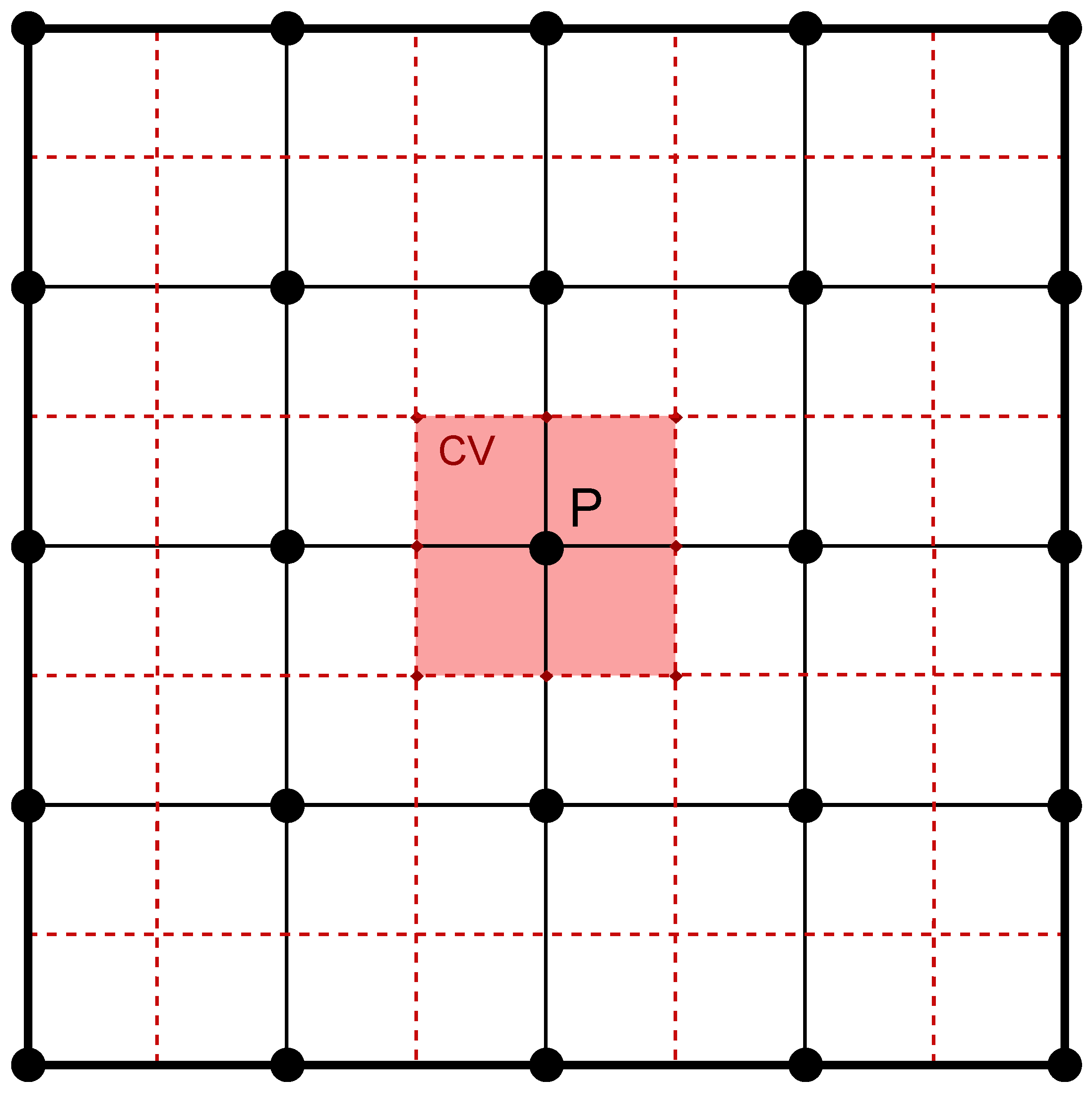
The finite-volume method (FVM) consists of subdividing the numerical domain into a finite and discrete number of control volumes (CV), over which the the governing equations are integrated, yielding the discretized equations at the CVs’ nodal points [27].
SU2 [21] uses the vertex-centered approach for variable arrangements, where the grid points are used as nodal points for the construction of the CV. Moreover, SU2 resorts to a median-dual technique, where the CVs are built around grid points by connecting the cells’ face-midpoints to the cell’s centroids. Consequently, a dual grid is generated. Figure 1 illustrates, in a simplified fashion, a primal grid designed by the user and then a dual grid composed by all the CVs and automatically generated by SU2.
The governing equations are integrated over the dual grid, where the Gauss Theorem is applied to the volume integrals associated with the convective and diffusive terms, converting them into surface integrals [21].
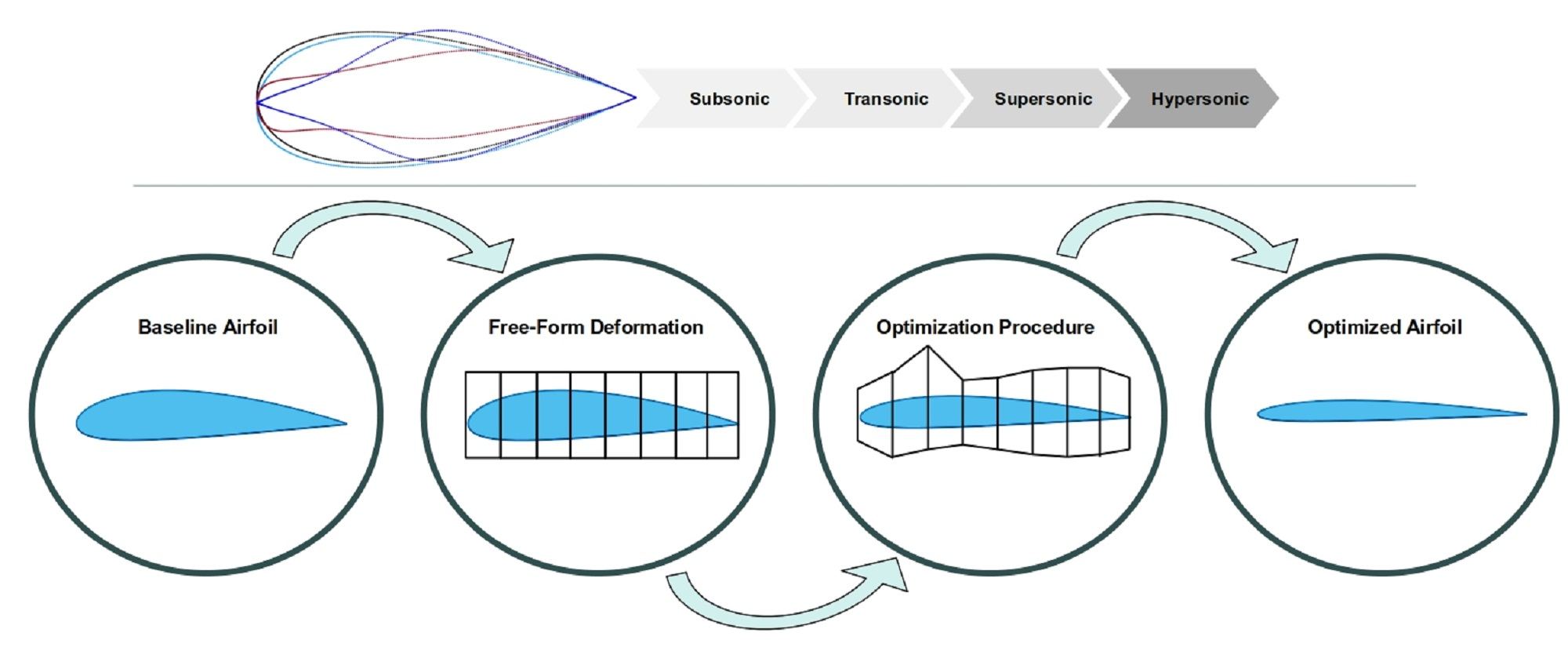
3. Methodology
Methodology comprises the strategies and steps undertaken throughout the present work in order to produce a feasible and accurate framework for both baseline and optimization simulations.
3.1. Airfoil Geometry & Mesh Design
The first step addresses the geometrical framework, that is, the set-up of the computational domain, which includes the airfoil geometry and the domain’s boundaries, followed by the mesh design and generation.
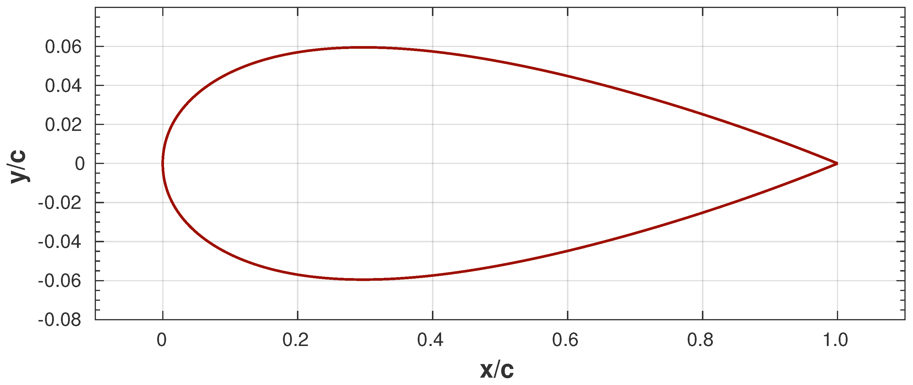
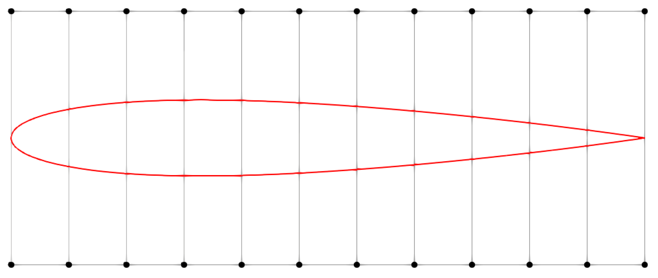
NACA0012, presented in Figure 2, is selected as the baseline geometry, given the great amount of experimental and numerical data available, as well as its worldwide use in validation and optimization problems. Note that, in Figure 2, and represent the x (chordwise direction) and y (thickness direction) coordinates of the airfoil geometry normalized to its chord, respectively. NACA0012 is a symmetrical airfoil; therefore, it has no camber and produces null lift at zero angle of attack (AoA). Its maximum thickness of 12% is located at 30% of the chord. In the present work, the airfoil coordinates are computed and then written in Gmsh [28] format using MATLAB.
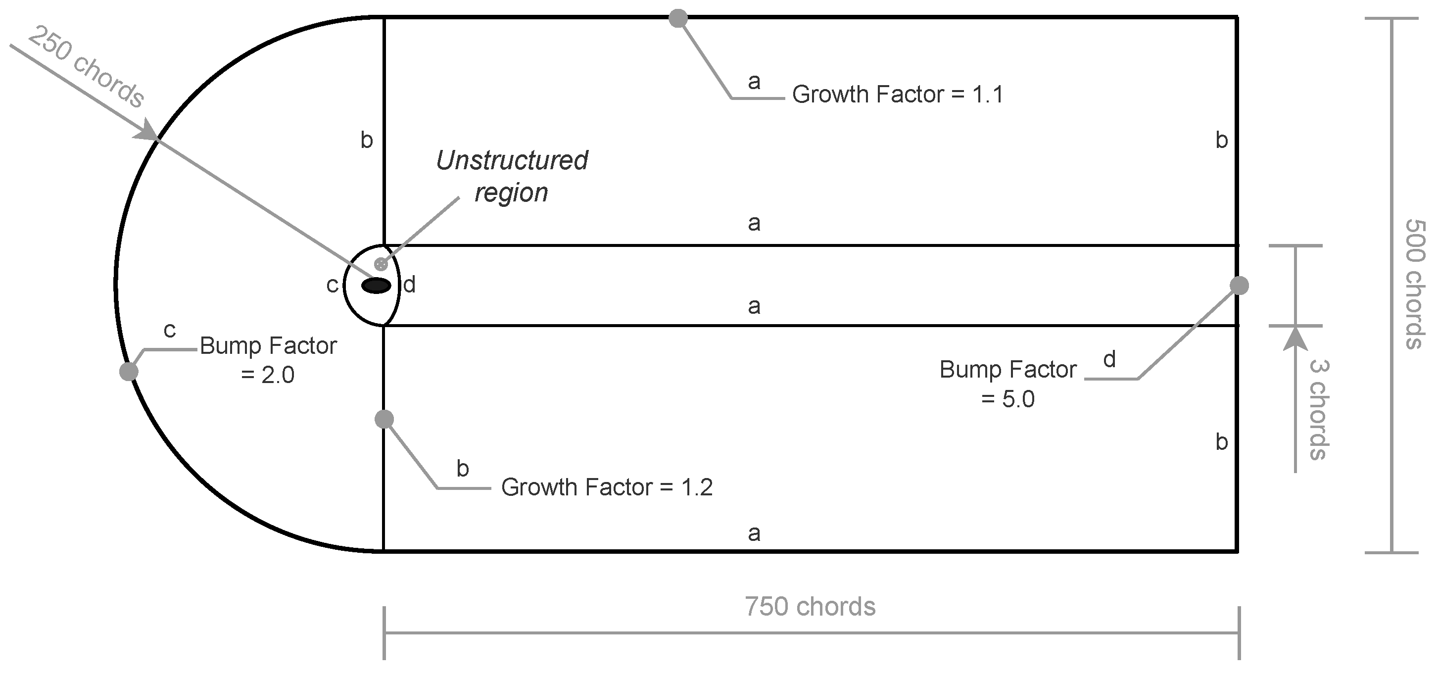
The design of the mesh is performed in Gmsh [28], open-source software with CAD-built capabilities. The meshing process takes into account several factors, including the airfoil geometry; the important physical phenomena that needs to be properly captured; the boundary conditions; and, finally, the computational cost. Moreover, mesh quality is guaranteed by ensuring smoothness, alignment, and low values of skewness throughout the mesh.
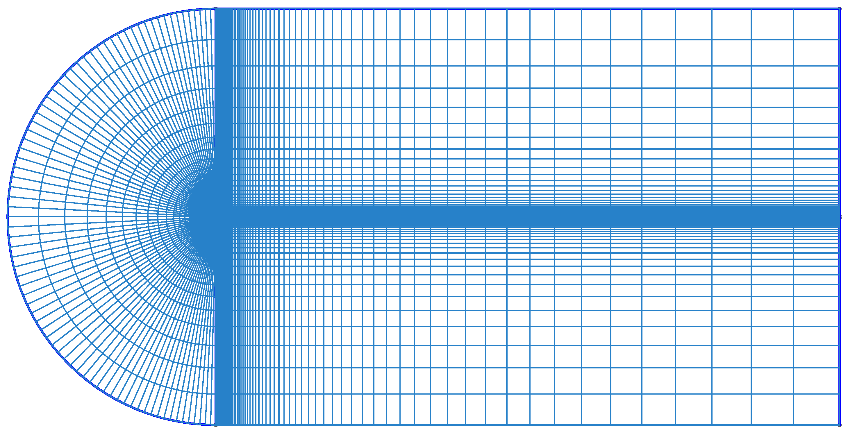
The overall structure of this work’s primal grid is displayed in Figure 3, containing information regarding the grid dimensions and growth factors. The grid is divided into five regions: one unstructured region surrounding the airfoil, and four structured regions enfolding the latter. The letters , and d denote the type of geometric factor (and its value) used to generate the mesh cells dimensions along the respective lines. For instance, lines marked with the letter a have cell dimensions built upon a geometric growth factor equal to 1.1 along the line direction. It is worth noting that those domain dimensions were chosen during the grid-convergence study, taking into account the four different flow regimes. The mesh employed in the present work is depicted in Figure 4, which corresponds to the medium mesh described below in Table 1.
3.2. Grid-Convergence Study (GCS)
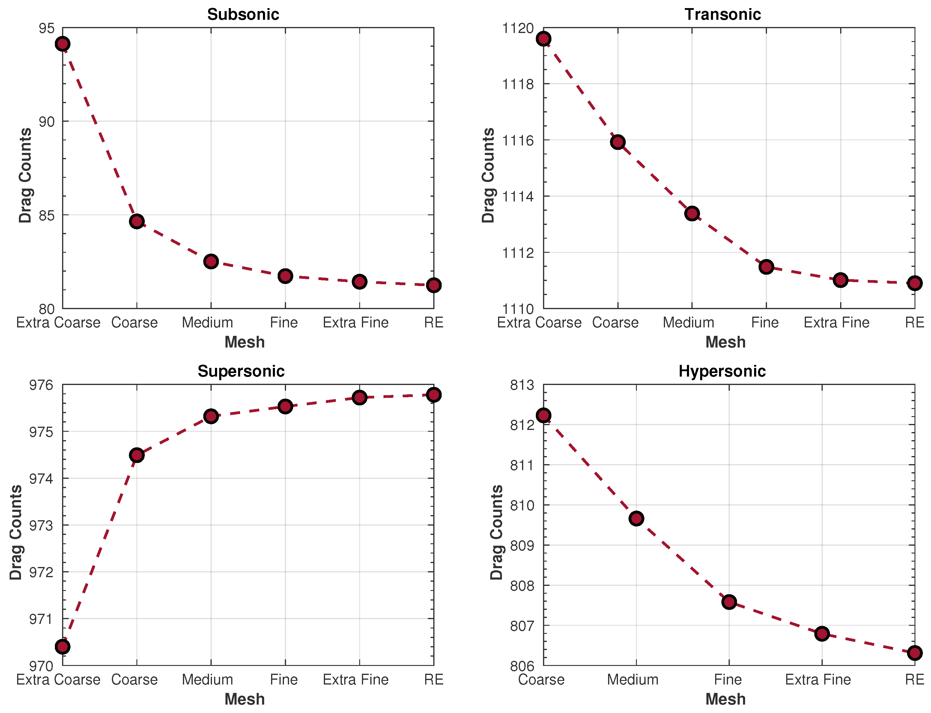
In order to ensure grid-independent numerical solutions and spatial convergence, a GCS is carried out for all speed regimes, from subsonic to hypersonic. In the present work, each study performs CFD steady-state simulations on five successively finer grids, depicted in Table 1. The grid refinement ratio, r, is equal to 2, and spatial convergence has been proved for all cases, as presented in Figure 5.
Furthermore, the Richardson extrapolation (RE) [29] method has been employed to obtain a higher-order estimate of the solution value when the grid spacing is equal to zero. This value is also presented in Figure 5, and the relative difference between the RE estimation and the value of the medium mesh is lower than 2% for all cases. Given the small relative difference and lower computational cost in comparison to finer grids, the medium mesh has been selected for the baseline and optimization simulations, with the exception of the hypersonic case, where the extra fine mesh is chosen due to convergence issues.
3.3. Baseline Simulations
Baseline simulations are steady-state CFD simulations performed for each of the different flight conditions. These simulations hold great importance since their numerical solutions—including aerodynamic data—are used as baseline comparison with respect to the optimization results.
In this work, four baseline simulations have been run in SU2 to assess the flow field and extract the main aerodynamic coefficients of NACA0012 airfoil at different flight conditions.
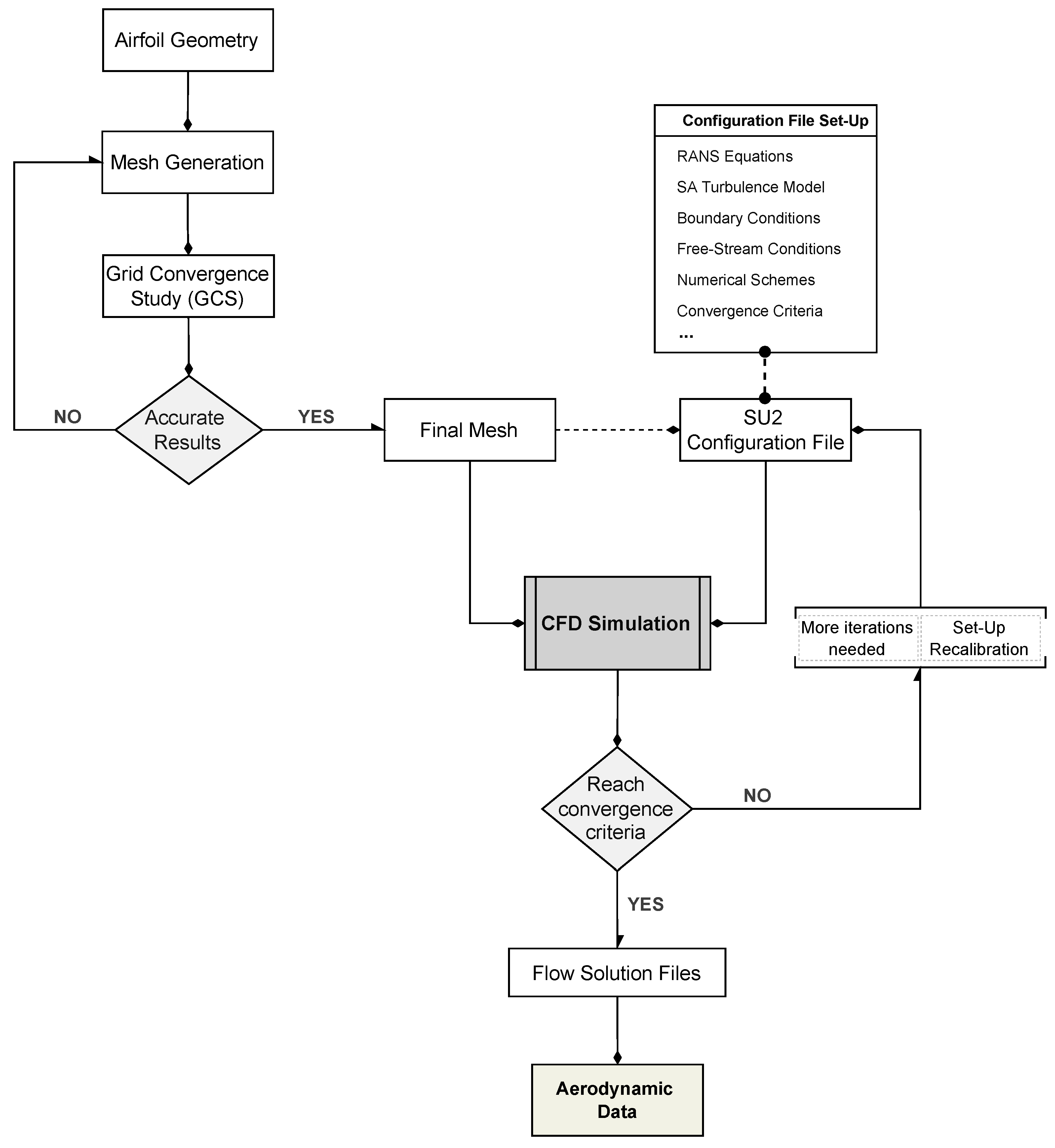
The flowchart with the detailed procedures to run such simulations is presented in Figure 6.
3.4. Optimization Simulations
One of the main objectives regarding the present work is to optimize the NACA0012 airfoil geometry so that better aerodynamic performance may be achieved for a given flight condition. Hence, a proper optimization framework is fundamental. The gradient-based method (GBM), developed within the SU2 framework, is applied to all speed regimes, from subsonic to hypersonic.
GBM are commonly employed in the design of aerospace vehicles, in which the vehicle shape—or airfoil shape in the case of the present work—is parameterized with a set of design variables. These methods compute the gradients of the objective function with respect to the design variables, thus defining better search directions and, ultimately, reaching an optimal design solution. The discrete adjoint method [30] is already implemented within SU2 and selected as GBM for an optimization procedure. Moreover, the free-form deformation (FFD) [31] parameterization technique is employed.
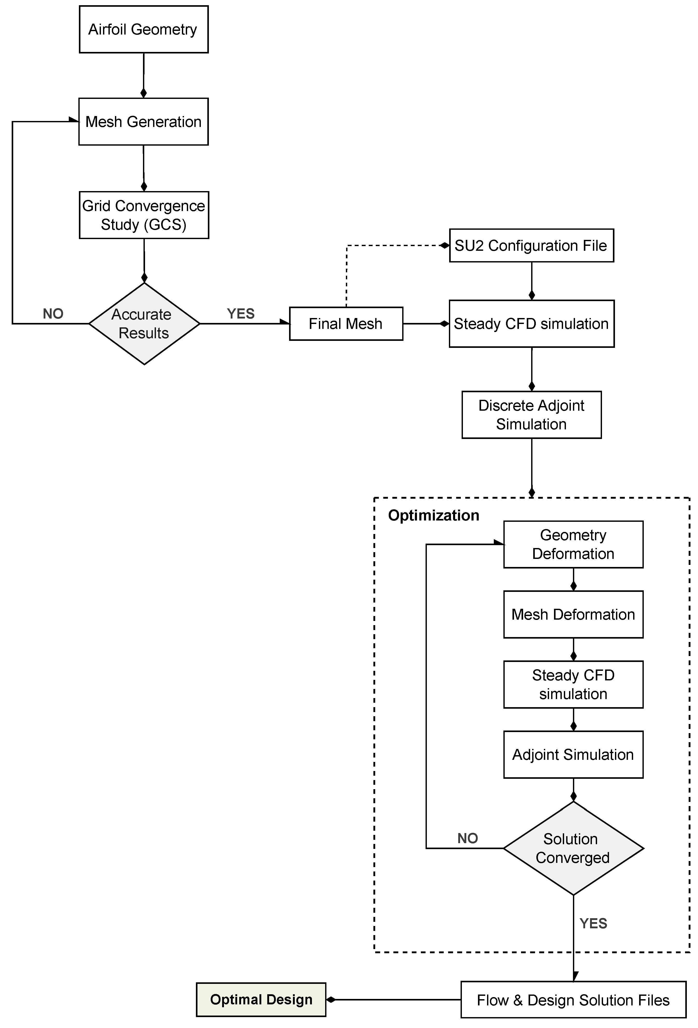
The flowchart containing the detailed gradient-based optimization procedure is illustrated in Figure 7.
Four optimization simulations have been carried out in SU2. Each of these optimizations corresponds to one of the selected points presented in Table 2. Regarding the parameterization technique, an FFD box has been wrapped around the airfoil geometry employing a total of 24 design variables equally spaced, as depicted in Figure 8.
The optimization formulation is presented below,
where the drag coefficient () is the objective function to be minimized, with respect to (w.r.t.) the 24 design variables X, and subject to (s.t.) a lift constraint and three airfoil geometrical constraints. Note that the LE radius refers to the radius of the leading edge. In addition to that, it is worth noting that those constraints were chosen during the grid-convergence study.
4. Problem Formulation
The goal is to assess and optimize the aerodynamic performance of two-dimensional NACA0012 airfoil for different speed regimes, within the framework of a hypothetical hypersonic transport aircraft.
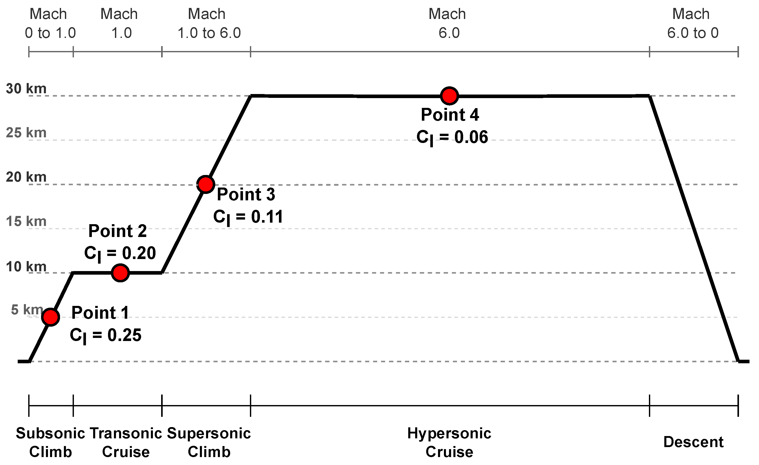
Mission Profile
The mission profile is presented below in Figure 9 and consists of a simplified description of the distinct flight segments, which are then associated with a given altitude and speed ranges. This mission profile has been produced in a similar fashion to the STRATOFLY [5] project’s mission profile.
As shown in Figure 9, four points have been selected to proceed with the analysis and optimization. The lift coefficient () values indicated on the figure are the target values for optimization, based on the mission profile of the STRATOFLY [5] project.
In Table 2, the main information with respect to each of these points is presented.
As one may observe, each of them represents a distinct speed regime, at different altitudes and temperatures. The Reynolds number () is greater than for all cases, thus stipulating that the flow is turbulent [20]. Moreover, the type of boundary condition (BC) applied in this work is presented below. The values of the Farfield BC vary in accordance to the free-stream properties of each flight condition. The Heat Flux BC is equal for all cases, indicating that the airfoil surface is an adiabatic, no-slip wall.
The convergence criterion for all the CFD simulations run in SU2 is the root mean square of the density residual. The threshold of convergence varies for each simulation case, depending on its speed regime, since convergence is more difficult to reach as the flow-speed increases. That said, the density residual must be lower than , , and for the subsonic, transonic, supersonic, and hypersonic cases, respectively. Moreover, the other residuals must also be inferior to .
5. Results and Discussion
The optimization results are addressed and compared to the baseline results. The optimal shapes are presented, as well as the pressure and temperature distributions along the chord. In the end, a morphing strategy is discussed.
5.1. Gradient-Based Optimizations
The results with respect to the main aerodynamic coefficients, and , are presented in Table 3. The first major difference is the production of lift by the optimized shapes, with the exception of the hypersonic case. The lift targets are satisfied for the subsonic, transonic, and supersonic cases. Moreover, with the production of lift, the optimized shapes present non-zero lift-to-drag ratio (L/D). The L/D comparison is presented below in Table 4, where for the subsonic case there is a large increase, and then, as expected, the L/D decreases with the increase in speed.
Regarding the drag coefficient, the results show a substantial decrease of 39.5%, 46.5%, and 79.2% in the transonic, supersonic, and hypersonic cases, respectively. The subsonic results show a small increase of 1.81%, which can be justified by the pressure drag caused by the generation of lift and due to the fact that NACA0012 is already a good shape for subsonic speeds.
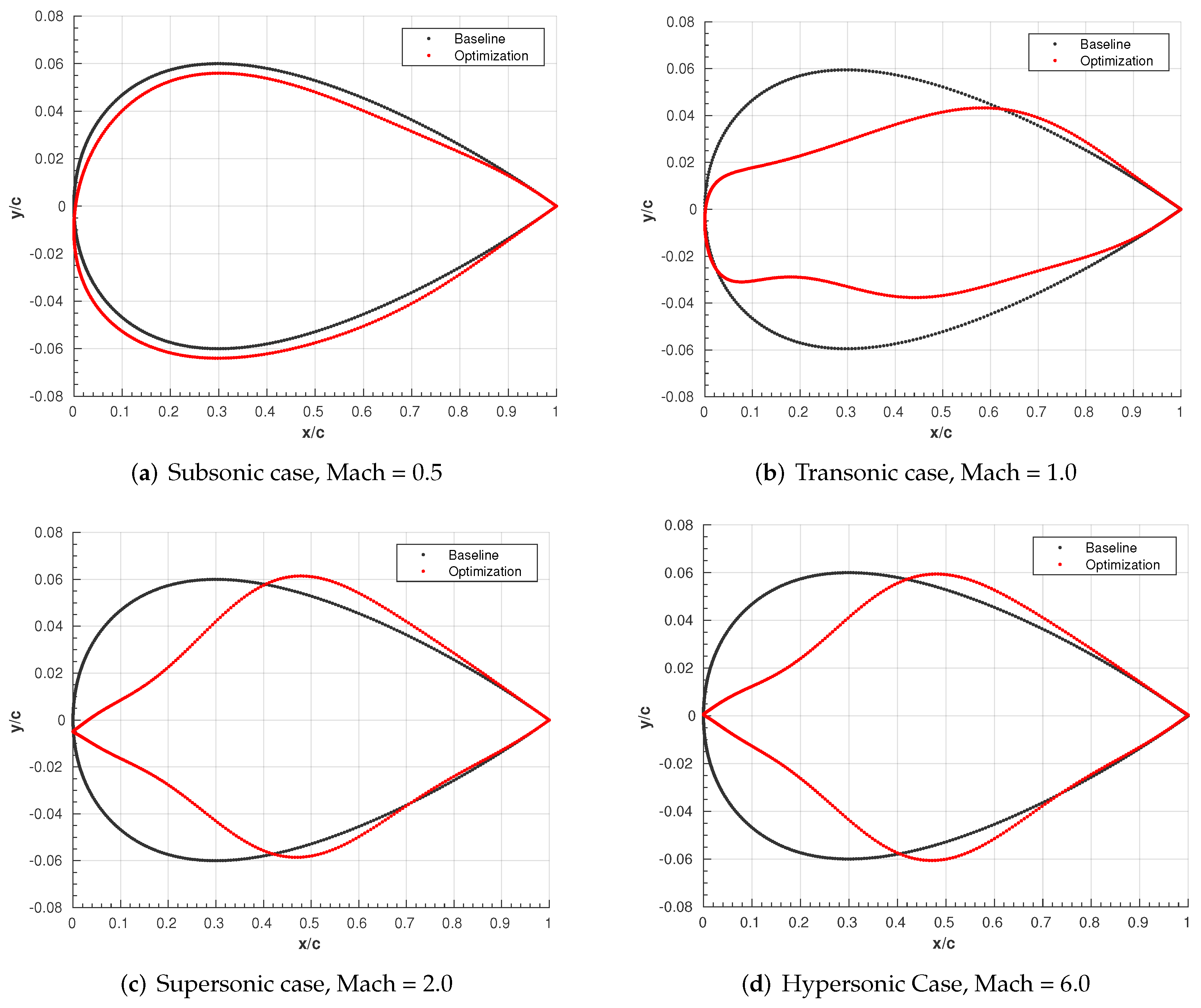
The comparison between the baseline and optimized shapes is presented in Figure 10. The subsonic results (Figure 10a) reinforce the statement that NACA0012 is a suitable geometry for low-speeds since its geometrical variation is very small. However, the transonic results show great differences in shape design between the optimization and baseline geometries (Figure 10b). The leading-edge region is stretched outwards and then, around , pushed a little inwards, resembling the shape of a whale.
Furthermore, there is a displacement of maximum thickness towards the back of the airfoil. Finally, in both the supersonic (Figure 10c) and hypersonic (Figure 10d) results, the optimal design greatly differs from the baseline one. The region comprising the leading edge is pulled inwards, significantly decreasing the LE radius. In addition to that, the position corresponding to the maximum thickness is moved from to , in both cases. These optimal designs resemble a biconvex or double wedge airfoil, which is expected for such high speeds [32].
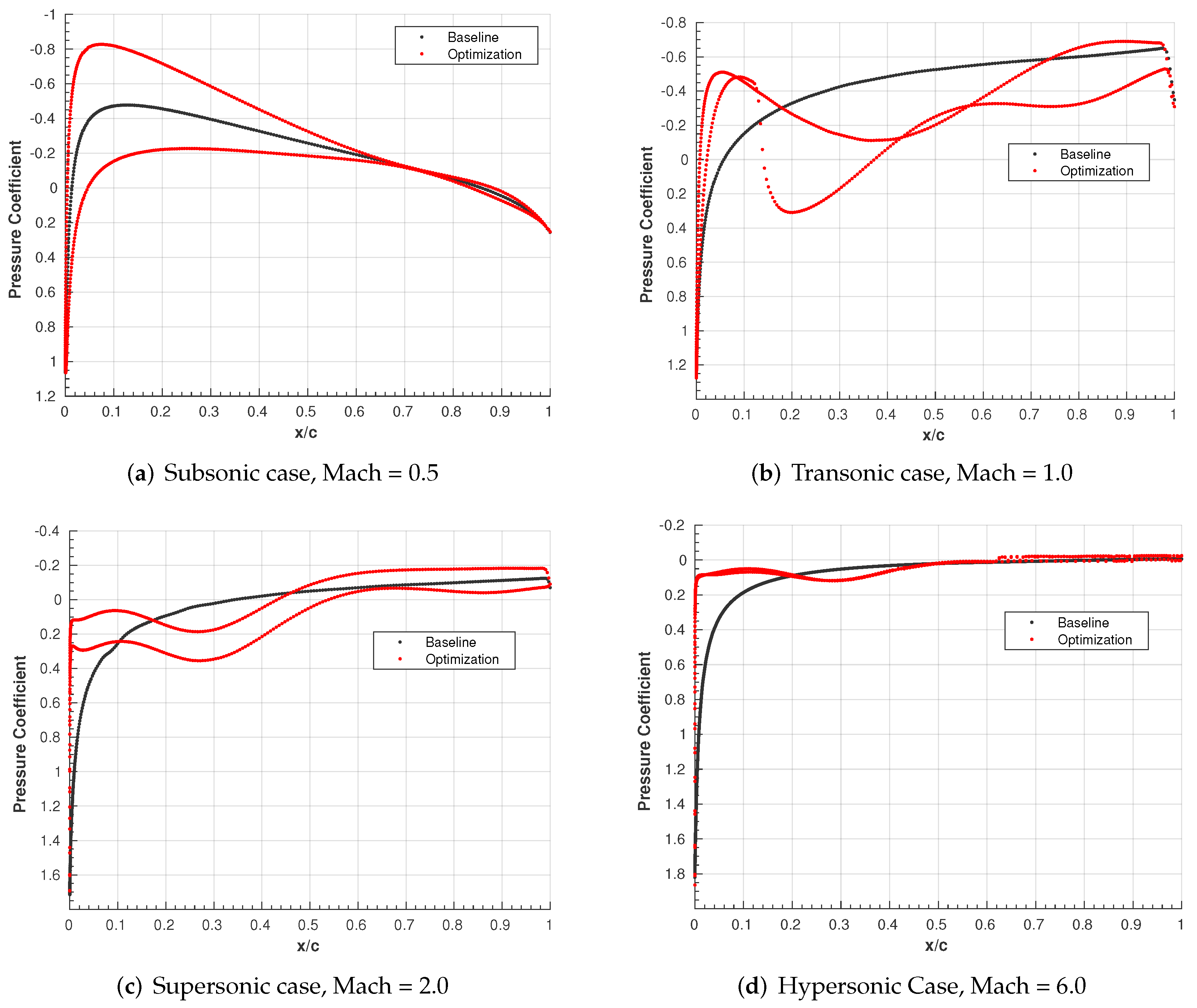
The distribution of the pressure coefficient, , along the chord is presented in Figure 11 for all cases. The baseline distributions display smooth behavior, where both the upper and lower surfaces show similar values of . However, as lift is generated by the optimized shapes, is expected to show differences between the upper and lower surfaces. These gaps are visible in the subsonic, transonic, and supersonic cases, as predicted. Moreover, it is important to point out that in both the transonic and supersonic cases, there are sudden variations of , mainly in the transonic case, which translates into the presence of shock waves. Nonetheless, the overall drag coefficient is still greatly reduced, as previously mentioned.
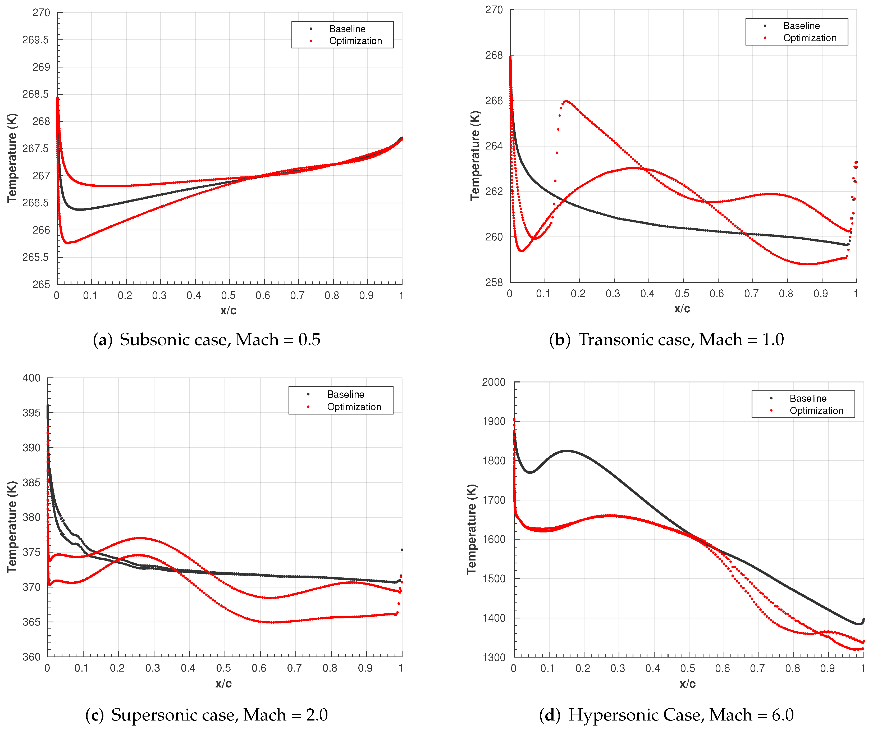
In the hypersonic environment, temperature plays an important role. A body subject to hypersonic speeds is confronted with very high temperatures, as well as great temperature gradients. These temperatures can be prejudicial to the body’s structural integrity and enable chemical reactions in the flow around, such as dissociation and ionization [32]. The temperature comparison between the baseline and optimization results is presented in Figure 12. The subsonic (Figure 12a), transonic (Figure 12b), and supersonic (Figure 12c) cases show small temperature variations between the upper and lower surfaces, and along . In addition to that, for the subsonic and transonic cases, temperatures are lower than 270 K, and for the supersonic case, lower than 400 K. However, this pattern significantly changes for the hypersonic case (Figure 12d), where temperatures reach a maximum of 1905.6 K at the stagnation point, and large variations—in the order of 600 K—take place along the airfoil surface. The lowest temperatures, around 1320 K, are observed at the trailing-edge region.
5.2. Morphing Strategy
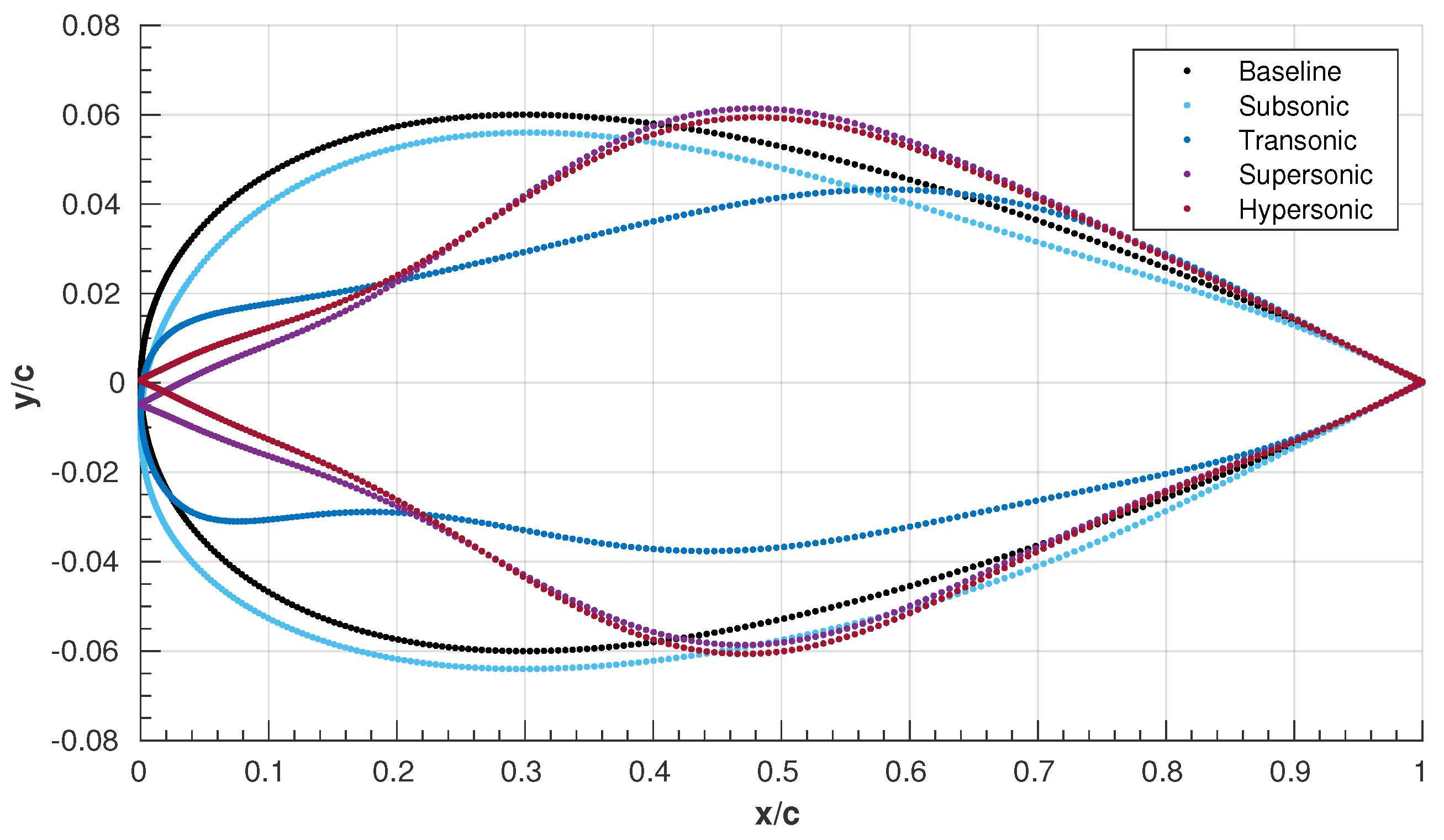
In Figure 13, the optimal designs with respect to the four flight points analyzed are compared between each other and to the NACA0012 baseline geometry. One may easily observe that the airfoil shape significantly changes as the speed regime increases and distances itself from the subsonic speeds. Therefore, in order to perform sufficiently well, or even excel, throughout the flight envelope, the airfoil shape must adapted.
By carefully observing Figure 13, it is possible to deduce two major tendencies, or patterns, essential to lay out a first morphing strategy. The first tendency observed refers to the airfoil thickness in the first third of the chord, . In this region, thickness is decreased as the speed increases from subsonic to hypersonic. Consequently, the maximum thickness is displaced to the right, near . In addition to that, the leading-edge radius also gets increasingly smaller as the speed increases, moving towards a biconvex-like shape. Therefore, a mechanism capable of pushing and pulling the surface within a certain degree would carry on the required changes.
The second pattern concerns the trailing-edge region, which exhibits almost no change throughout the optimizations for the distinct flight conditions. Therefore, it is possible, and even advantageous structure-wise, to fix part of the airfoil geometry.
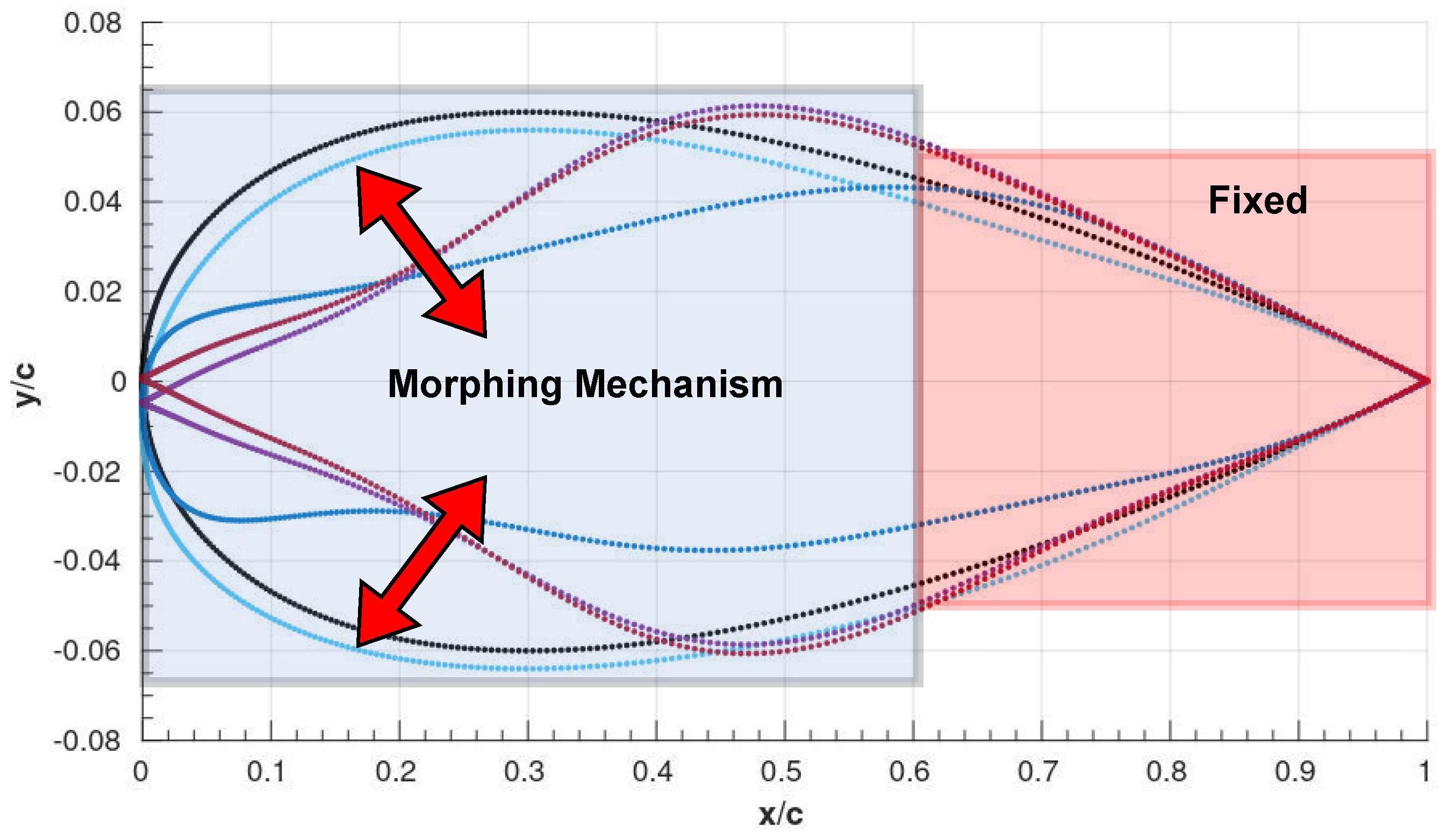
The final morphing strategy presented in Figure 14 establishes two regions: one fixed sector starting from , associated with the airfoil’s aft region, including the trailing edge, and one movable region, where an eventual elastic skin of the airfoil may be pushed both in- and outwards to satisfy the design requirement of a given flight point.
6. Conclusions
The present work presents the development of a computational framework that optimizes a lifting surface over a full range of speeds from subsonic to hypersonic flight regimes. The framework is based on a high-fidelity computational fluid dynamics analysis coupled with an optimization algorithm that morphs the airfoil geometry into an optimal design for the specific flight conditions and constraints. The optimization process results in a drag reduction of up to 79.2%. Lift requirements have also been satisfied for all flight points, except for the hypersonic case, which should be further investigated.
Author Contributions
Conceptualization, B.L., F.A. and A.S.; methodology, B.L. and F.A.; software, B.L.; validation, B.L., F.A.; formal analysis, B.L., F.A.; investigation, B.L., F.A., A.S.; data curation, B.L. and F.A.; writing—original draft preparation, B.L.; writing—review and editing, F.A. and A.S.; visualization, B.L.; supervision, F.A. and A.S.; and project administration, A.S. All authors have read and agreed to the published version of the manuscript.
Funding
The authors acknowledge Fundação para a Ciência e a Tecnologia (FCT), through IDMEC, under LAETA, project UIDB/50022/2020.
Informed Consent Statement
Not applicable.
Data Availability Statement
The data presented in this study are available on request.
Conflicts of Interest
The authors declare no conflict of interest.
Abbreviations and Acronyms
The following abbreviations and acronyms are used in this manuscript:
| ASO | Aerodynamic shape optimization |
| BC | Boundary condition |
| CAD | Computer-aided design |
| CFD | Computational fluid dynamics |
| CV | Control volumes |
| DNS | Direct numerical solution |
| FFD | Free-form deformation |
| FVM | Finite-volume method |
| GBM | Gradient-based method |
| GCS | Grid-convergence study |
| ICAO | International Civil Aviation Organization |
| PDE | Partial differential equations |
| RANS | Reynolds-averaged Navier–Stokes |
| SA | Spalart–Allmaras |
| SU2 | Standford University Unstructured |
| Nomenclature | |
| Convective fluxes | |
| Viscous fluxes | |
| Velocity vector | |
| State variables vector | |
| Design variables | |
| Dynamic viscosity | |
| Density | |
| Shear-stress tensor | |
| Drag coefficient | |
| Lift coefficient | |
| L/D | Lift-to-drag ratio |
| Identity matrix | |
| E | Total energy |
| H | Total enthalpy |
| k | Thermal conductivity |
| p | Pressure |
| Q | Source term |
| r | Grid-refinement ratio |
| Reynolds number | |
| T | Temperature |
| c | Airfoil chord |
| K | Kelvin |
| s.t. | Subject to |
| w.r.t. | With respect to |
| x | x-coordinate |
| y | y-coordinate |
References
- ICAO Annual Report. Available online: https://www.icao.int/annual-report-2019/Documents/ARC_2019_Air%20Transport%20Statistics.pdf (accessed on 24 April 2021).
- Liu, F.; Han, Z.; Zhang, Y.; Song, K.; Song, W.; Gui, F.; Tang, J. Surrogate-based aerodynamic shape optimization of hypersonic flows considering transonic performance. Aerosp. Sci. Technol. 2019, 93, 105345. [Google Scholar] [CrossRef]
- Periodic Reporting for Period 1—STRATOFLY. Available online: https://cordis.europa.eu/project/id/769246/reporting/it (accessed on 18 June 2021).
- Taguchi, H.; Kobayashi, H.; Kojima, T.; Ueno, A.; Imamura, S.; Hongoh, M.; Harada, K. Research on hypersonic aircraft using pre-cooled turbojet engines. Acta Astronaut. 2012, 73, 164–172. [Google Scholar] [CrossRef]
- Viola, N.; Fusaro, R.; Saracoglu, B.; Schram, C.; Grewe, V.; Martinez, J.; Marini, M.; Hernandez, S.; Lammers, K.; Vincent, A.; et al. Main Challenges and Goals of the H2020 STRATOFLY Project. Aerotec. Missili Spaz. 2021, 10, 95–110. [Google Scholar] [CrossRef]
- Bowcutt, K.G. Stratospheric Flying Opportunities for High-Speed Propulsion Concepts: Hypersonic Vehicle Design Challenges. In Proceedings of the von Karman Institute for Fluid Dynamics—Lecture Series, Online, 25–27 May 2021. [Google Scholar]
- Skinner, S.N.; Zare-Behtash, H. State-of-the-art in aerodynamic shape optimisation methods. Appl. Soft Comput. 2018, 62, 933–962. [Google Scholar] [CrossRef]
- Jameson, A. Aerodynamic design via control theory. J. Sci. Comput. 1988, 3, 233–260. [Google Scholar] [CrossRef] [Green Version]
- Liu, B.; Liang, H.; Han, Z.-H.; Yang, G. Surrogate-based aerodynamic shape optimization of a morphing wing considering a wide Mach-number range. Aerosp. Sci. Technol. 2022, 124, 107557. [Google Scholar] [CrossRef]
- Ma, Y.; Yang, T.; Feng, Z.; Zhang, Q. Hypersonic lifting body aerodynamic shape optimization based on the multiobjective evolutionary algorithm based on decomposition. Proc. Inst. Mech. Eng. Part J. Aerosp. Eng. 2015, 229, 1246–1266. [Google Scholar] [CrossRef]
- Peng, W.; Feng, Z.; Yang, T. Rapid Aerodynamic Shape Optimization With Payload Size Constraints for Hypersonic Vehicle. IEEE Access 2019, 7, 84429–84447. [Google Scholar] [CrossRef]
- Martins, J.R.R.A. Aerodynamic design optimization: Challenges and perspectives. Comput. Fluids 2022, 239, 105391. [Google Scholar] [CrossRef]
- Mangano, M.; Martins, J.R.R.A. Multipoint Aerodynamic Shape Optimization for Subsonic and Supersonic Regimes. J. Aircr. 2021, 58, 650–662. [Google Scholar] [CrossRef]
- Reuther, J.; Alonso, J.J.; Rimlinger, M.J.; Jameson, A. Aerodynamic shape optimization of supersonic aircraft configurations via an adjoint formulation on distributed memory parallel computers. Comput. Fluids 1999, 28, 675–700. [Google Scholar] [CrossRef] [Green Version]
- Jim, T.M.S.; Faza, G.A.M.; Palar, P.S.; Shimoyama, K. Bayesian Optimization of a Low-Boom Supersonic Wing Planform. AIAA J. 2021, 59, 4514–4529. [Google Scholar] [CrossRef]
- Deng, F.; Jiao, Z.-h.; Chen, J.; Zhang, D.; Tang, S. Overall Performance Analysis–Oriented Aerodynamic Configuration Optimization Design for Hypersonic Vehicles. J. Spacecr. Rocket. 2017, 54, 1015–1026. [Google Scholar] [CrossRef]
- Seraj, S.; Martins, J.R. Aerodynamic Shape Optimization of a Supersonic Transport Considering Low-Speed Stability. In Proceedings of the AIAA SCITECH 2022 Forum, San Diego, CA, USA, 3–7 January 2022. [Google Scholar] [CrossRef]
- Weisshaar, T.A. Morphing Aircraft Systems: Historical Perspectives and Future Challenges. J. Aircr. 2013, 50, 337–353. [Google Scholar] [CrossRef]
- Li, D.; Zhao, S.; Da Ronch, A.; Xiang, J.; Drofelnik, J.; Li, Y.; Zhang, L.; Wu, Y.; Kintscher, M.; Monner, H.P.; et al. A review of modelling and analysis of morphing wings. Prog. Aerosp. Sci. 2018, 100, 46–62. [Google Scholar] [CrossRef] [Green Version]
- Anderson, J.D. Fundamentals of Aerodynamics, 5th ed.; McGraw-Hill: New York, NY, USA, 2011. [Google Scholar]
- Economon, T.D.; Palacios, F.; Copeland, S.R.; Lukaczyk, T.W.; Alonso, J.J. SU2: An Open-Source Suite for Multiphysics Simulation and Design. AIAA J. 2016, 54, 828–846. [Google Scholar] [CrossRef]
- Moukalled, F.; Mangani, L.; Darwish, M. The Finite Volume Method in Computational Fluid Dynamics; Springer: Cham, Swizerland, 2016. [Google Scholar] [CrossRef] [Green Version]
- Kolmogorov, A.N. The local structure of turbulence in incompressible viscous fluid for very large Reynolds numbers. Proc. R. Soc. Math. Phys. Eng. Sci. 1991, 434, 9–13. [Google Scholar] [CrossRef]
- Spalart, P.; Allmaras, S. A one-equation turbulence model for aerodynamic flows. In Proceedings of the 30th Aerospace Sciences Meeting and Exhibit, Reno, NV, USA, 6–9 January 1992. [Google Scholar] [CrossRef]
- Nemec, M.; Zingg, D.W.; Pulliam, T.H. Multipoint and Multi-Objective Aerodynamic Shape Optimization. AIAA J. 2004, 42, 1057–1065. [Google Scholar] [CrossRef]
- Waligura, C.J.; Couchman, B.L.; Galbraith, M.C.; Allmaras, S.R.; Harris, W.L. Investigation of Spalart-Allmaras Turbulence Model Modifications for Hypersonic Flows Utilizing Output-Based Grid Adaptation. In Proceedings of the AIAA SCITECH 2022 Forum, San Diego, CA, USA, 3–7 January 2022. [Google Scholar] [CrossRef]
- Versteeg, H.K.; Malalasekera, W. An Introduction to Computational Fluid Dynamics: The Finite Volume Method, 2nd ed.; Pearson Education Limited: Harlow, UK, 2007. [Google Scholar]
- Geuzaine, C.; Remacle, J.-F. Gmsh: A 3-D finite element mesh generator with built-in pre- and post-processing facilities. Int. J. Numer. Methods Eng. 2009, 79, 1309–1331. [Google Scholar] [CrossRef]
- Richardson, L.F. IX. The approximate arithmetical solution by finite differences of physical problems involving differential equations, with an application to the stresses in a masonry dam. Proc. R. Soc. Math. Phys. Eng. Sci. 1911, 210, 307–357. [Google Scholar] [CrossRef] [Green Version]
- Nadarajah, S.; Jameson, A. A comparison of the continuous and discrete adjoint approach to automatic aerodynamic optimization. In Proceedings of the 38th Aerospace Sciences Meeting and Exhibit, Reno, NV, USA, 10–13 January 2000. [Google Scholar] [CrossRef] [Green Version]
- Sederberg, T.; Parry, S. Free-form deformation of solid geometric models. In Proceedings of the 13th Annual Conference on Computer Graphics and Interactive Techniques, Dallas, TX, USA, 18–22 August 1986. [Google Scholar] [CrossRef]
- Anderson, J.D. Hypersonic and High-Temperature Gas Dynamics, 2nd ed.; American Institute of Aeronautics and Astronautics: Reston, VA, USA, 2006. [Google Scholar]
Figure 1.
Illustration of both the primal grid (black continuous line) and dual grid (red dashed line).
Figure 1.
Illustration of both the primal grid (black continuous line) and dual grid (red dashed line).

Figure 2.
NACA 0012 airfoil geometry.

Figure 3.
Overall mesh strategy and dimensions.

Figure 4.
Mesh generation.

Figure 5.
GCS for the four speed regimes.

Figure 6.
Baseline simulation flowchart.

Figure 7.
Gradient-based optimization flowchart.

Figure 8.
FFD box.

Figure 9.
Mission profile.

Figure 10.
Comparison between baseline and optimized airfoil shapes. (a) Subsonic case, Mach = 0.5. (b) Transonic case, Mach = 1.0. (c) Supersonic case, Mach = 2.0. (d) Hypersonic Case, Mach = 6.0.
Figure 10.
Comparison between baseline and optimized airfoil shapes. (a) Subsonic case, Mach = 0.5. (b) Transonic case, Mach = 1.0. (c) Supersonic case, Mach = 2.0. (d) Hypersonic Case, Mach = 6.0.

Figure 11.
Comparison between baseline and optimized pressure coefficient distributions. (a) Subsonic case, Mach = 0.5. (b) Transonic case, Mach = 1.0. (c) Supersonic case, Mach = 2.0. (d) Hypersonic case, Mach = 6.0.
Figure 11.
Comparison between baseline and optimized pressure coefficient distributions. (a) Subsonic case, Mach = 0.5. (b) Transonic case, Mach = 1.0. (c) Supersonic case, Mach = 2.0. (d) Hypersonic case, Mach = 6.0.

Figure 12.
Comparison between baseline and optimized temperature distributions. (a) Subsonic case, Mach = 0.5. (b) Transonic case, Mach = 1.0. (c) Supersonic case, Mach = 2.0. (d) Hypersonic case, Mach = 6.0.
Figure 12.
Comparison between baseline and optimized temperature distributions. (a) Subsonic case, Mach = 0.5. (b) Transonic case, Mach = 1.0. (c) Supersonic case, Mach = 2.0. (d) Hypersonic case, Mach = 6.0.

Figure 13.
Baseline and optimized airfoil design geometries: overlap and comparison.

Figure 14.
Final morphing strategy.


Table 1.
Information regarding the five grids used for the GCS.
| Mesh | Mesh Elements |
|---|---|
| Extra Coarse | 19,864 |
| Coarse | 40,276 |
| Medium | 89,335 |
| Fine | 217,890 |
| Extra Fine | 604,804 |
Table 2.
Main information regarding selected points.
| Point | Speed Regime | Mach | Altitude | Temperature | Reynolds Number |
|---|---|---|---|---|---|
| 1 | Subsonic | 0.5 | 5 km | 255.65 K | 7.25 × |
| 2 | Transonic | 1.0 | 10 km | 223.25 K | 8.49 × |
| 3 | Supersonic | 2.0 | 20 km | 216.65 K | 3.69 × |
| 4 | Hypersonic | 6.0 | 30 km | 226.65 K | 2.26 × |
Table 3.
Comparison between baseline and gradient-based optimization aerodynamic coefficients.
| Point | Speed Regime | Baseline | Optimization | Baseline | Optimization | (%) | |
|---|---|---|---|---|---|---|---|
| 1 | Subsonic | 0.00 | 0.25 | +0.25 | 0.008407 | 0.008559 | +1.81% |
| 2 | Transonic | 0.00 | 0.20 | +0.20 | 0.111338 | 0.067349 | −39.5% |
| 3 | Supersonic | 0.00 | 0.11 | +0.11 | 0.097532 | 0.052138 | −46.5% |
| 4 | Hypersonic | 0.00 | 0.00 | 0.00 | 0.080679 | 0.016742 | −79.2% |
Table 4.
Lift-to-drag ratio results.
| Point | Speed Regime | Lift-to-Drag (L/D) Baseline | Lift-to-Drag (L/D) Optimization |
|---|---|---|---|
| 1 | Subsonic | 0.00 | 29.20 |
| 2 | Transonic | 0.00 | 2.97 |
| 3 | Supersonic | 0.00 | 2.69 |
| 4 | Hypersonic | 0.00 | 0.00 |
Publisher’s Note: MDPI stays neutral with regard to jurisdictional claims in published maps and institutional affiliations. |
© 2022 by the authors. Licensee MDPI, Basel, Switzerland. This article is an open access article distributed under the terms and conditions of the Creative Commons Attribution (CC BY) license (https://creativecommons.org/licenses/by/4.0/).
Share and Cite
MDPI and ACS Style
Leite, B.; Afonso, F.; Suleman, A. Aerodynamic Shape Optimization of a Symmetric Airfoil from Subsonic to Hypersonic Flight Regimes. Fluids 2022, 7, 353. https://0-doi-org.brum.beds.ac.uk/10.3390/fluids7110353
AMA Style
Leite B, Afonso F, Suleman A. Aerodynamic Shape Optimization of a Symmetric Airfoil from Subsonic to Hypersonic Flight Regimes. Fluids. 2022; 7(11):353. https://0-doi-org.brum.beds.ac.uk/10.3390/fluids7110353
Chicago/Turabian StyleLeite, Bernardo, Frederico Afonso, and Afzal Suleman. 2022. "Aerodynamic Shape Optimization of a Symmetric Airfoil from Subsonic to Hypersonic Flight Regimes" Fluids 7, no. 11: 353. https://0-doi-org.brum.beds.ac.uk/10.3390/fluids7110353