
A Direct-Forcing Immersed Boundary Method for Incompressible Flows Based on Physics-Informed Neural Network


1
The State Key Laboratory of Nonlinear Mechanics, Institute of Mechanics, Chinese Academy of Sciences, Beijing 100190, China
2
School of Engineering Science, University of Chinese Academy of Sciences, Beijing 100049, China
*
Author to whom correspondence should be addressed.
Fluids 2022, 7(2), 56; https://0-doi-org.brum.beds.ac.uk/10.3390/fluids7020056
Submission received: 2 December 2021
/
Revised: 11 January 2022
/
Accepted: 13 January 2022
/
Published: 25 January 2022
(This article belongs to the Collection Feature Paper for Mathematical and Computational Fluid Mechanics)
Abstract
:The application of physics-informed neural networks (PINNs) to computational fluid dynamics simulations has recently attracted tremendous attention. In the simulations of PINNs, the collocation points are required to conform to the fluid–solid interface on which no-slip boundary condition is enforced. Here, a novel PINN that incorporates the direct-forcing immersed boundary (IB) method is developed. In the proposed IB-PINN, the boundary conforming requirement in arranging the collocation points is eliminated. Instead, velocity penalties at some marker points are added to the loss function to enforce no-slip condition at the fluid–solid interface. In addition, force penalties at some collocation points are also added to the loss function to ensure compact distribution of the volume force. The effectiveness of IB-PINN in solving incompressible Navier–Stokes equations is demonstrated through the simulation of laminar flow past a circular cylinder that is placed in a channel. The solution obtained using the IB-PINN is compared with two reference solutions obtained using a conventional mesh-based IB method and an ordinary body-fitted grid method. The comparison indicates that the three solutions are in excellent agreement with each other. The influences of some parameters, such as weights for different loss components, numbers of collocation and marker points, hyperparameters in the neural network, etc., on the performance of IB-PINN are also studied. In addition, a transfer learning experiment is conducted on solving Navier–Stokes equations with different Reynolds numbers.
1. Introduction
Over the past few years, machine learning (ML) has permeated into various research areas of fluid mechanics [1], e.g., reduced-order modeling [2,3], wake-type clustering and classification [4,5,6,7], development of turbulence closure model [8,9,10], flow optimization and active control [11,12,13,14,15,16], to name a few. The successful application of ML to these areas relies on the availability of large-scale data, which are obtained from CFD simulations or experimental observations.
More recently, the physics-informed neural network (PINN) was proposed to solve partial differential equations (PDEs) [17,18,19]. PINNs use automatic differentiation to compute the derivatives, and the residuals of equations are incorporated into the loss function. Unlike the conventional practice in ML, PINN can be trained without any simulation (or observation) data or with only a small amount of data. Nowadays, PINN has been successfully applied to the simulations of incompressible [20,21,22,23] and compressible [24] flows.
PINN is not meant to be a replacement of traditional CFD solvers but instead a complementary approach. For solving a standard forward problem (one PDE system with fixed parameters), the state-of-art PINN cannot compete with the traditional CFD methods in terms of accuracy, efficiency and robustness. However, a surrogate model based on PINN is a good choice in some non-ideal situations where traditional CFD methods cannot handle or are very expensive to use, such as data assimilation with numerical solution, solving ill-posed problems due to a lack of boundary conditions and solving inverse problems. Other advantages of PINN include: (a) closed-form approximated solutions with continuous derivatives, (b) implementation simplicity on high-level marching learning platforms.
PINN can be regarded as a mesh-free method for solving PDEs since an explicit mesh is not needed. In PINN, the no-slip condition at the fluid–solid interface is imposed by incorporating velocity penalties at the boundary points into the loss function. As that in traditional mesh-based numerical methods, the boundary points are required to conform to the surfaces of immersed objects.
The immersed boundary (IB) method is an alternative technique for handling complex and moving boundaries in mesh-based methods. It utilizes non-boundary-conforming meshes in numerical discretization, and the no-slip condition on the surface of the immersed object is enforced by adding a volume force to the momentum equation. This method has recently gained its popularity due to the simplicity of implementation.
The combination of PINN and the IB method can eliminate the boundary-conforming requirement in point generation. This eases the point generation process in problems with complex boundaries and avoids redistributing the points in moving-boundary problems. These benefits motivate the development of a novel PINN in conjunction with the IB method in this work. Such benefits were also the main motivation for incorporating IB method into a smoothed particle hydrodynamics (SPH) flow solver [25]. The proposed IB-PINN can be considered a complementary approach to the classical (mesh-based) IB schemes (rather than a replacement). Here, we emphasize that the mesh-free nature of PINN can barely be considered a potential advantage in such a combination. This is because mesh generation in the mesh-based IB method is significantly simplified and not a challenging task anymore.
To the best of the authors’ knowledge, PINNs, in conjunction with IB method, are still barely explored. Balam et al. recently presented a PINN for solving two-dimensional elliptic equations with singular forces on an embedded interface [26]. The IB method involved in their work fell into the ’continuous-forcing’ sub-type. The forcing terms in the equations were explicitly computed via a jump condition at the interface, together with a smoothed delta function for spreading the singular force. Thus, no major modification to the original framework of PINN was needed in their work.
In this paper, we consider the ‘direct-forcing’ sub-type of IB methods. Unlike the one in [26], in this variant of IB methods, the forcing term is determined indirectly via a no-slip constraint imposed on the embedded interface. Due to the lack of an explicit expression for the forcing term, the loss components that account for the equation residual and non-slip condition on the embedded interface need to be reformulated.
The paper is organized as follows. In Section 2, we present an introduction to the direction-forcing IB method and the architecture of neural network used in this study. The results of the simulations using the proposed IB-PINN are presented in Section 3. Finally, the summary of the present work and suggestions on future directions are provided in Section 4.
2. Methods
2.1. Direct-Forcing Immersed Boundary Method
We consider the incompressible Navier–Stokes equations with a volume force added to the momentum equation. The governing equations can be written in a dimensionless form as:
where is the Reynolds number, , p and denote the velocity, pressure, volume force (density), respectively. The spatial variable denotes the position in the computational domain (which includes the region occupied by the immersed object). represents an embedded fluid–solid interface. s is the coordinate along the interface for parameterizing it. represents the singular force that is added to the fluid–solid interface. Equation (3) is the formula for the transfer between the surface force and the volume force. Equation (4) is the no-slip constraint that must be satisfied at the surface of a stationary object.
For incompressible Navier–Stokes equations, the pressure p acts as a set of Lagrange multipliers, which enforce the divergence-free condition (Equation (2)). In direct-forcing IB methods, the surface (and volume) forces can also be regarded as a set of Lagrange multipliers that enforce the no-slip condition (Equation (4)) on the embedded interface. In numerical implementations, the forcing term and pressure can be obtained sequentially [27,28] or simultaneously in a coupled way [29,30] via splitting the system (Equations (1)–(4)).
In conventional mesh-based discretization, , p and are defined at the grid points, while is defined at a set of marker points that represent the interface. The integral operations in Equations (3) and (4) are replaced by summation, and the delta function is replaced by a smoothed delta function with compact support [31].
2.2. Physics-Informed Neural Network
Instead of using conventional mesh-based methods, in this work, a deep neural network (DNN) is used to approximate the solution of incompressible Navier–Stokes equations. The architecture of the DNN used here is similar to those proposed in some previous references [17,20,21,22] (see Figure 1). The DNN is composed of multiple hidden layers, and it can be expressed as:
where denotes the hidden variables of the ℓth layer, and and denote the weight matrix and bias vector of the ℓth layer, respectively. is a nonlinear activation function. Throughout this work, the hyperbolic tangent function is used as the activation function. The Xavier initialization technique is used to initialize the network [32]. The DNN takes the spatial-temporal variables as the inputs. The outputs of the last layer are used to approximate the solution . Please note that the surface force , which is an auxiliary variable for obtaining the volume force in some mesh-based IB methods, is not used here. The DNN is implemented using the TensorFlow machine learning platform, and the source code can be found in https://github.com/huangyi89/IB-PINN (accessed 12 January 2022).
PINN solves a PDE system by converting it into an optimization problem in which the loss function is minimized through iteratively updating the weights and biases. Generally speaking, the total loss for a PDE system is composed of equation residual loss, initial condition loss and boundary condition loss. In solving a PDE system in the framework of direct-forcing IB methods, special care needs to be taken in constructing the loss component associated with the non-slip boundary condition at the embedded interface. In this study, we propose incorporating velocity penalties at some marker points that represent the embedded interface into the total loss. Obtaining the forcing term by adding a velocity penalty to the loss function is analogous to obtaining the pressure by adding the residual of the continuity equation into the loss function in the PINNs proposed by Sun et al. [20] and Jin et al. [21]. This analogy is rooted in the fact that both the forcing term and pressure are Lagrangian multipliers for imposing constraint on the system [29,30]. In addition to the velocity penalty term, the total loss in the proposed IB-PINN also includes a force penalty term that is used to ensure compact distribution of volume force. To this end, the force penalties are applied at the collocation points, which are exterior to and beyond certain distance from the immersed interface. The compact distribution of the forcing term is a necessary condition for accurately mimicking the dynamic effect of an immersed object on fluid flow. In conventional mesh-based IB methods, such a condition is automatically satisfied by using an interpolation kernel function (i.e., smoothed delta function) with compact support [31].
As a result, the loss function used for training IB-PINN can be expressed as:
Here J denotes the total loss function, which is the summation of four components corresponding to the residual loss (), the outer boundary loss (), the boundary loss associated with the immersed boundary () and the force compactness loss (). As a proof-of-concept, only steady problems are considered in this work. Thus, the initial condition loss is neglected in Equation (6). , , and are the weights for the aforementioned four loss components, respectively.
The equation residual loss can be further decomposed into the loss for the momentum Equation () and the loss for the continuity Equation (). In computing the equation residual loss, the partial differential operations are performed using automatic differentiation (AD). and denote the velocity and pressure that are specified on the outer boundaries, respectively. and denote the numbers of collocation points and marker points, respectively. and denote the numbers of boundary points where velocity and pressure are specified, respectively. denotes the number of collocation points on which force penalties are applied.
The locations of the three sets of points, namely collocation points, boundary points and marker points, are illustrated in Figure 2. The collocations points are located inside the computational domain (including the area occupied by the immersed object) and on the outer boundary. The boundary points are located on the outer boundary where data for velocity or pressure are available. In this work, the boundary points and the collocation points coincide with each other on the outer boundary. Such a choice of boundary points is just for the simplicity of implementation. A different set of boundary points that does not belong to the collocation points can also be chosen [26]. The marker points are located inside the domain for representing the fluid–solid interface (i.e., immersed boundary). Please note that the marker points do not belong to the set of collocation points and are only used for computing the loss. The force penalties are applied at the collocations points that are located in the gray area (the area outside the cylinder and beyond a distance of Δ from the immersed boundary). Please note that no force penalties are applied at the collocation points that lie inside the immersed object.
3. Results
3.1. Problem Description and Numerical Settings
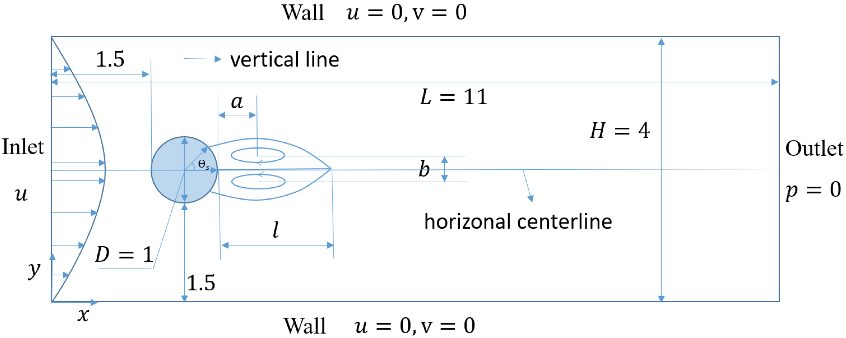
We use the proposed IB-PINN to simulate fluid flow past a circular cylinder that is placed in a channel [22]. Since only a steady case is considered here, the Reynolds number based on the diameter of the cylinder is set to 40, which is below the critical value for the onset of vortex shedding. The computational domain and boundary conditions are illustrated in Figure 3. At the inlet, a parabolic profile of the streamwise velocity is specified, and the crosswise velocity component is set to zero. Mathematically, the parabolic velocity profile is defined as
where H denotes the height of the channel. At the outlet, the pressure is set to zero. The no-slip condition is imposed on the top and bottom walls of the channel.
A total of 72,365 collocation points (with 2564 outer boundary points) and 251 marker points are used in the simulation. The collocation points are placed at the vertices of a uniformly distributed Cartesian mesh with a grid width of h = 0.025. Please note that this mesh is generated for arranging the collocation points only and is not used explicitly in the IB-PINN simulations. The marker points are uniformly distributed on the surface of the cylinder. As a usual practice in IB methods, the spacing between two neighboring marker points is comparable with that between two neighboring collocation points. The distance Δ in Figure 2, which represents the supporting width of volume force, is set to 2 h.
The DNN used in the simulations is composed of six hidden layers, of which the number of layer neurons is 100. The weights for the loss components are: λ = 1.0; α = 2.0; β = 2.0; γ = 1.0. In the training process, we follow the strategy adopted in some previous works, such as [21,22], where certain numbers of iterations are first performed using the Adam optimizer; after that, the L-BFGS-B optimizer is used to finetune the DNN to obtain a more accurate solution. In this work, 104 iterations in the Adam optimizer are first performed with a fixed learning rate of 5 × 10⁻⁴ before the L-BFGS-B optimizer is used. The training with the L-BFGS-B optimizer is terminated based on the increment tolerance (or if the total number of iterations reaches 105). The training is performed on Tesla-V100 16G/32G GPU.
A reference solution is obtained by using a conventional mesh-based IB method. This numerical method is based on the discrete stream-function formulation for solving incompressible Navier–Stokes equations [28]. The spatial discretization and temporal advancement in the flow solver are of second-order accuracy. For detailed descriptions and validations of the mesh-based IB method, please refer to [28,33,34]. The uniform rectangular mesh aforementioned (with h = 0.025) is used in the simulation. The smoothed delta function used in the mesh-based IB method has a supporting width of 4 h (the half supporting width is equal to Δ) [35].
An additional reference solution is also obtained by performing a simulation using Ansys Fluent. This software uses an ordinary CFD method (with body-fitted mesh and velocity-pressure formation). The resolution of the simulation is comparable with that of the mesh-based IB method. The numerical settings of this simulation are described in Appendix A.
3.2. Predicted Solution vs. Reference Solutions
The convergence history of the training process is shown in Figure 4. It is seen that after the training is terminated, the total loss is reduced to a value less than 4 × 10⁻⁵, while the maximum value among the four loss components is around 2 × 10⁻⁵. The low values of the final loss indicate the convergence of training.
The contours of the streamwise and crosswise velocity components obtained using Fluent, mesh-based IB method and IB-PINN are displayed in Figure 5. The contours for the difference between the two IB solutions are also shown in the figure. The comparisons indicate that the three solutions are in excellent agreement qualitatively. Actually, an evident difference does exist in the interior of the cylinder between the solutions of the two IB methods. However, the interior flows in IB methods are merely fictitious and irrelevant to the prediction accuracy. Thus, in plotting the difference between the two IB solutions, data for the interior flows are removed, and the interior regions are filled with white color.
The streamlines for the three solutions are shown in Figure 6. Again, it is seen that the flow fields exterior to the cylinder are in excellent agreement. Evident difference in the fictitious flows obtained by the two IB methods can be visualized in the interior of the cylinder. This difference is mainly due to the fact the force compactness constraint is imposed inside the cylinder in the mesh-based IB method but not in IB-PINN.
The profiles of streamwise velocity along the horizontal centerline and vertical line passing through the center of the cylinder are shown in Figure 7. The quantitative agreement between the three solutions can be seen clearly. Again, larger discrepancies are only found on the segment inside the cylinder (corroding to the region where fictitious flows are produced in the two IB methods).
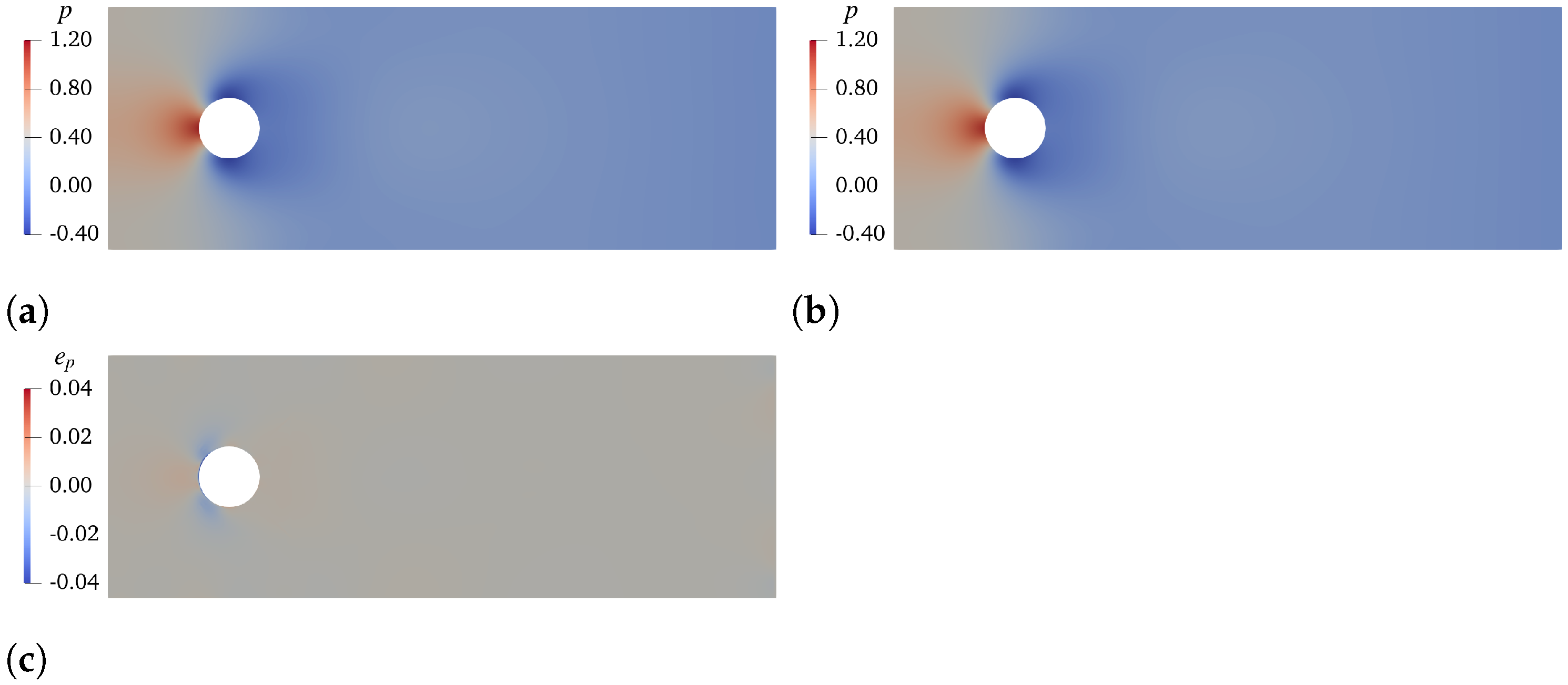
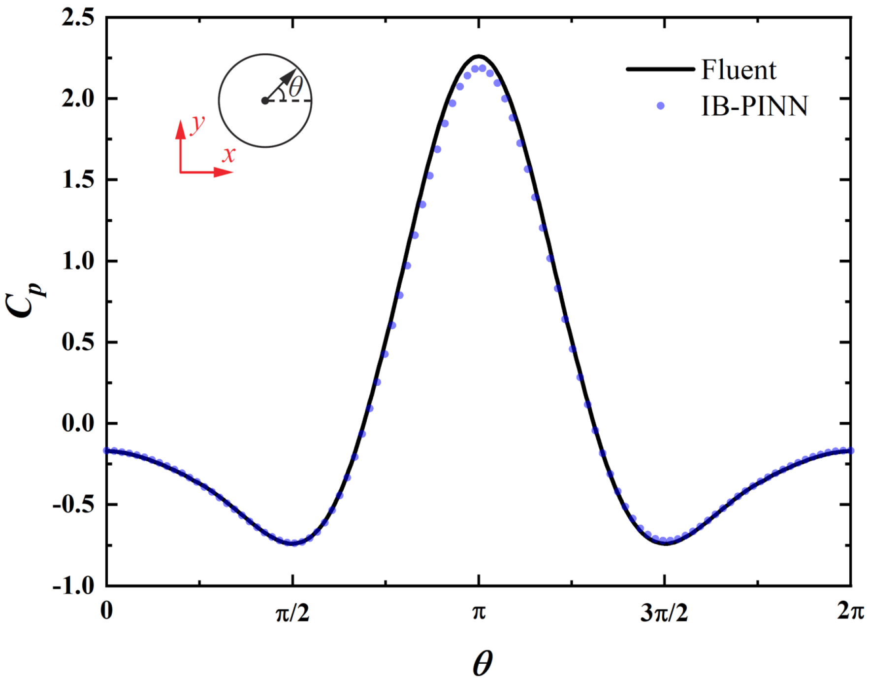
The pressure contours obtained using IB-PINN and Fluent are compared in Figure 8. The distributions of the pressure coefficient along the cylinder surface are also compared in Figure 9. A good agreement between the two solutions is clearly demonstrated. The slight under-prediction of the pressure coefficient near the front stagnation point in IB-PINN is associated with the smearing effect of diffusive-interface IB methods. The pressure prediction in IB-PINN can be improved by adopting a local refinement strategy in the generation of collocation points. Here, the pressure field for the mesh-base IB method is not available. This is because the mesh-based IB solver is based on the discrete stream-function formulation in which the pressure is eliminated.
The length and position of the separation bubble behind the cylinder, the separation angle and the drag coefficient are listed in Table 1 for comparison. For the IB methods, the drag coefficient is computed by
where denotes the x-component of volume force ; , and D are (non-dimensional) density, maximum velocity and diameter, respectively, (i.e., ). For the solution of Fluent, the drag coefficient is computed by the integration of pressure and friction forces on the cylinder surface. From this table, it can be seen that the results from the three simulations also agree very well.
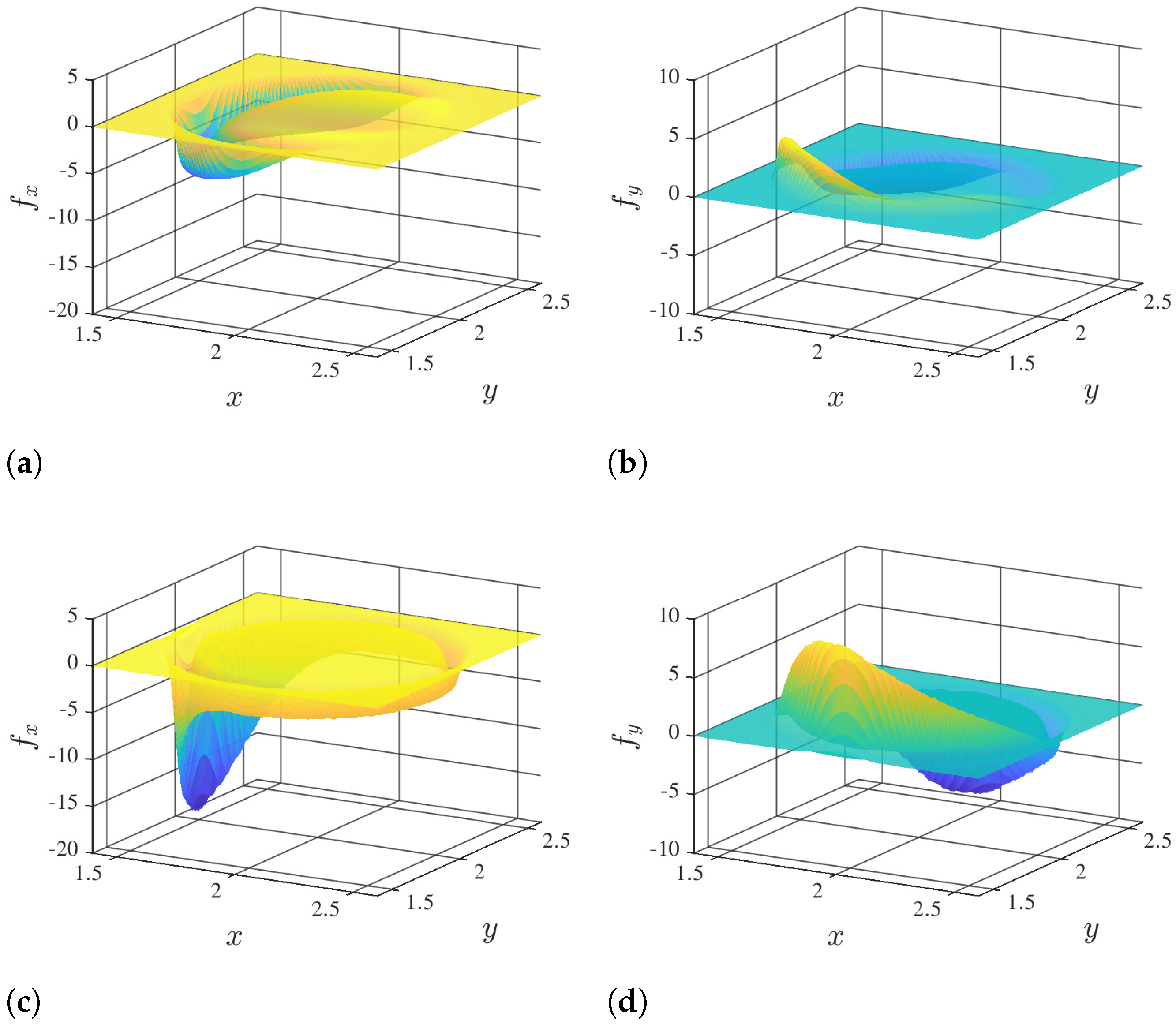
The distributions of the volume force obtained in the two simulations of IB methods are compared in Figure 10. It is interesting to note that although the velocity fields obtained in the two simulations are very similar, the two volume forces differ significantly. The dissimilarity in the distributions of volume force is partially due to the lack of the force compactness constraint inside the cylinder in the IB-PINN simulation. Another reason for the discrepancy between the two volume forces is that no interpolation kernel function is used in IB-PINN, while in the mesh-based IB method, an interpolation kernel function is used to regulate the distribution of volume force.
3.3. Influences of Some Parameters on the Performance of IB-PINN
In this section, we study how the performance of IB-PINN is affected by the variations of some parameters. The IB-PINN with the numerical settings aforementioned is regarded as the baseline model to compare with. The value of final loss after training and the relative error of velocity are used to quantify the convergence behavior and prediction accuracy, respectively. Here, the relative error is defined as
where represents the two velocity components obtained by IB-PINN. represents an accurate solution, which is obtained using the conventional IB method, on a very fine mesh of h = 0.005. Please note that the fictitious velocity inside the circular cylinder is excluded in the computation of relative error.
The effects of the DNN architecture on the convergence of training and velocity error are tested by using DNNs with nine different configurations. To be more specific, three numbers of hidden layers (5, 6, 7) and three numbers of neurons per layer (90, 100, 110) are considered. The results obtained by the nine DNNs are summarized in Table 2. The low values of final loss indicate good convergence in training all DNNs. As to the prediction accuracy, the smallest velocity error is achieved in DNN with 6 hidden layers and 100 neurons per layer. This implies that for a fixed number of collocation points, a DNN with a more complex architecture (i.e., larger size) does not necessarily provide a more accurate prediction. Similar findings were also reported in some previous studies on PINNs [20,21,22,26].
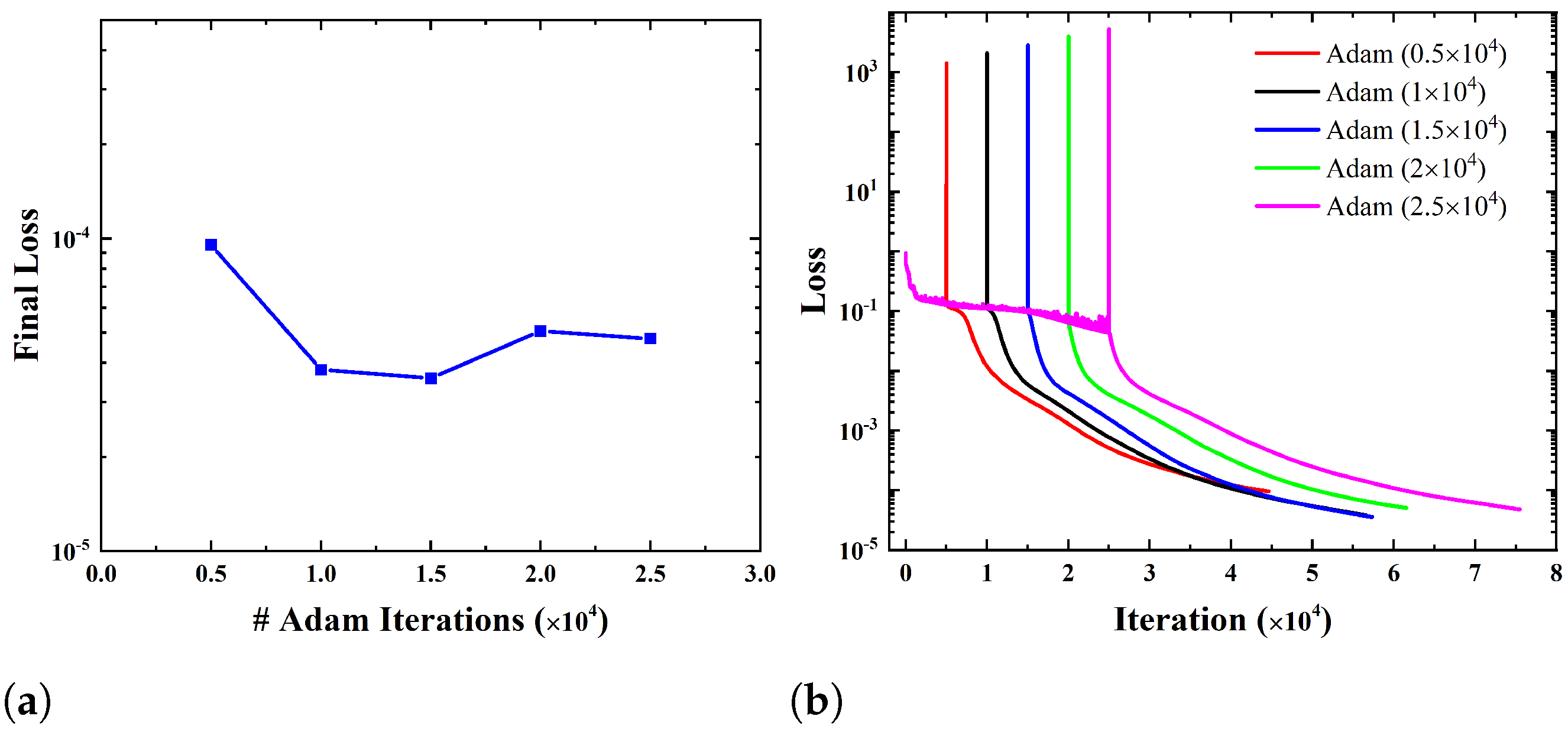
Figure 11 shows the influence of the number of Adam iterations (before L-BFGS-B) on the convergence of training. From Figure 11a, it is seen that the final loss is not very sensitive to the number of Adam iterations. A low value of final loss (less than 5 × 10⁻⁵) can be achieved if the number of Adam iterations lies in the range of 1.0 × 10⁴ to 2.5 × 10⁴. From the convergence histories shown in Figure 11b, it can be seen that a much larger loss declining rate can be achieved in the L-BFGS-B optimizer in comparison with the Adam optimizer. However, since L-BFGS-B is a local optimizer, a certain number of iterations in Adam is necessary at the beginning to avoid becoming stuck on the local optimum. To keep the total number of iterations (in both optimizers) as small as possible while maintaining a low final loss, 1.0 × 10⁴ iterations in Adam before switching to L-BFGS-B is an appropriate choice. Due to the non-convexness of the loss function in this study, optimization can get stuck in local minima in a few cases with certain numbers of collocation points. It is found that the optimization can escape the local minima by adjusting the number of Adam iterations.
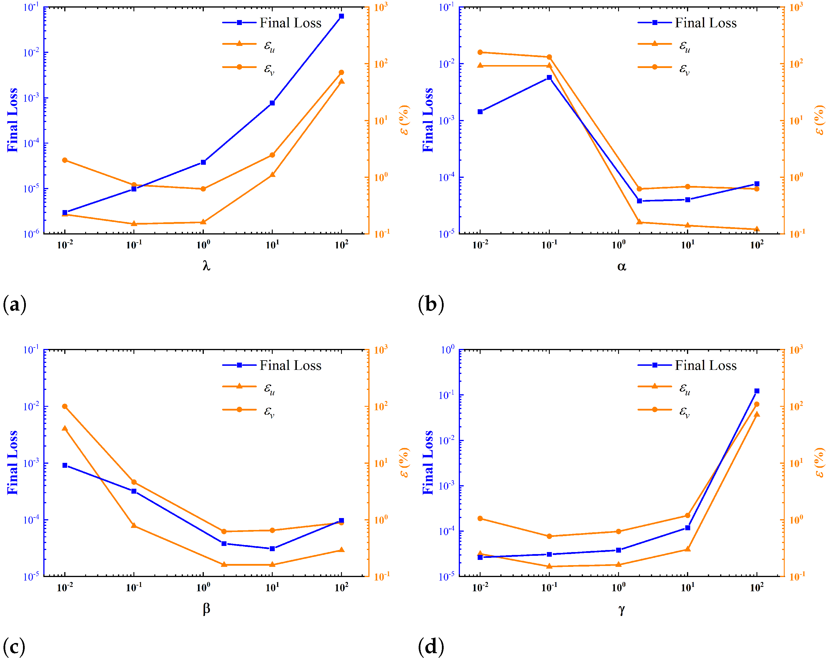
The effects of four weights in the loss function on the convergence of training and prediction accuracy are tested by changing one weight once a time while keeping the other three fixed. The influences of the weights on the value of the final loss and prediction error are shown in Figure 12. It is seen that choosing appropriate weights is crucial for ensuring the convergence of training and achieving high accuracy in prediction. A rule that provides guidance to the selection of weights can be easily inferred from the figure. If it is required that the low final loss is less than 1.0 × 10⁻⁴ and the relative velocity errors are less than 1%, and should lie in range of [0.1, 1.0], while and should lie in the range of [2.0, 100.0].
The interpretations of the optimized ranges of weights observed in this figure are as follows. First, weights much larger than one should be assigned to the boundary losses. This is because the boundary losses are usually one order of magnitude smaller than the other two loss components in the training process. Small weights for the boundary losses can result in the domination of equation and force components in the total loss. This makes the optimization hard to converge since the boundary conditions are never properly satisfied. Second, when the weights for the PDE and force losses are too small, a prediction error rises even if the training converges very well. Here, the large discrepancy between predicted and true solutions is linked with the violations of the governing equation and force compactness condition.
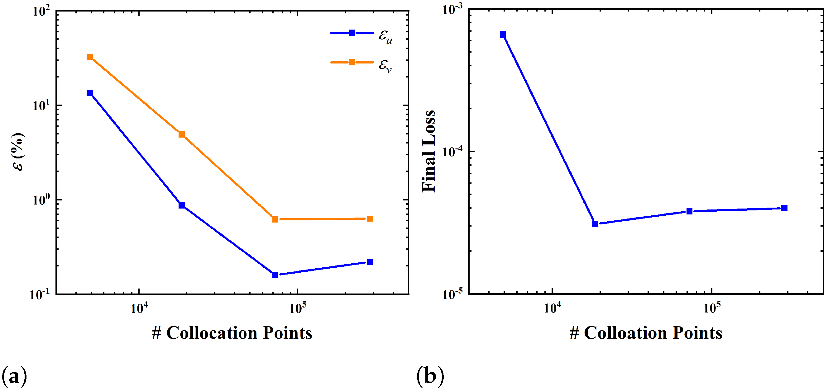
The convergence of the prediction error with respect to the number of collocation points is also examined. In the refinement and coarsening process, auxiliary rectangular meshes with different resolutions are generated for arranging the collocation points. The variation of the velocity error with the number of collocation points is shown in Figure 13a. It is seen that with the increasing number of collocation points, an (almost) converged solution can be reached when the number of collocation points is larger than 7.2 × 10⁴. The relative velocity errors in the converged solution are in the order of 10−3 to 10−2. If the number of collocation points is increased further from 7.2 × 10⁴, the prediction error almost levels off (even increases slightly). This can be explained by the fact that the prediction accuracy is ultimately limited by the optimization error in training the DNN if the number of collocation points becomes sufficiently large. The supporting evidence for this explanation can be found in Figure 13b. It is seen that the value of final loss does not change significantly if the number of collocation points is larger than 1.8 × 10⁴.
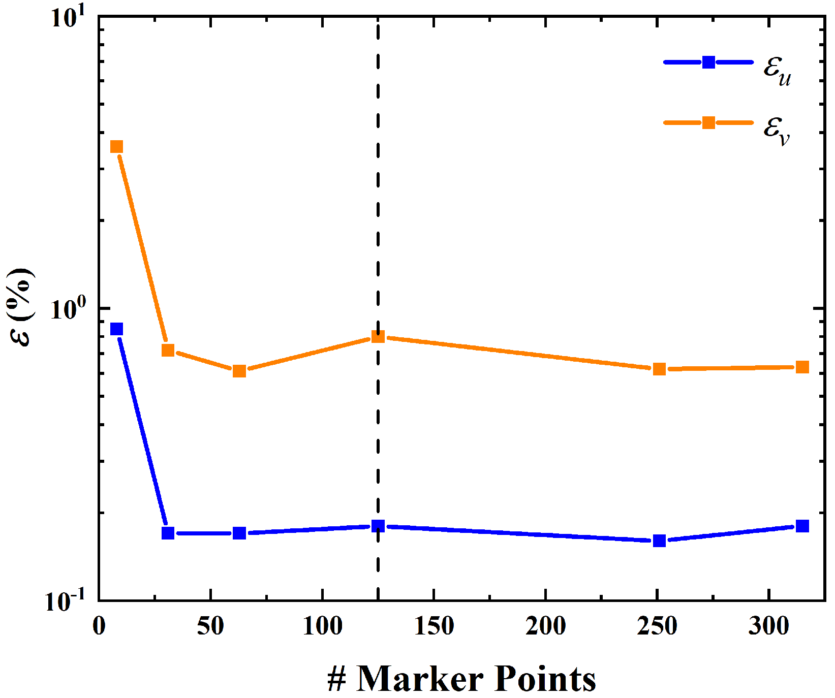
Similarly, the effect of the number of marker points on the prediction accuracy is tested by changing the number of marker points from 8 to 314 while keeping the number of collocation points fixed to 7.2 × 10⁴. From Figure 14, it is seen that the prediction accuracy is less sensitive to the number of marker points. Thus, the requirement of marker-point resolution for representing the cylinder surface is not very stringent. In this test, 125 marker points on the cylinder surface correspond to a resolution that is compatible with that of the collocation points. However, 31 marker points are sufficient for achieving an accurate prediction.
The influence of imposing a force compactness constraint inside the cylinder is also examined. In other words, force penalties are also applied to the collocation points that are in the interior of the cylinder and beyond a distance of Δ from the immersed boundary. We notice that in the mesh-based IB method used for obtaining the reference solution, half of the support in the interpolation kernel function lies inside the cylinder and spans a width of Δ. Thus, the distribution of volume force in the IB-PINN with such a constraint is supposed to be more akin to that in the mesh-based IB method. The final loss, velocity errors and drag coefficient obtained by IB-PINNs with and without such a constraint are compared in Table 3. It is seen that imposing such a constraint makes the training process hard to converge and thus leads to a much larger prediction error.
3.4. Transfer Learning
In the current setting of IB-PINN, we only consider solving Navier–Stokes equations with a fixed Reynolds number. For a prediction at a different Reynolds number, the DNN needs to be re-trained. The large re-training overhead is an inherent drawback that severely limits its application in optimization problems.
Transfer learning is a powerful technique in machine learning to accelerate convergence and save training time. In transfer learning, a base network is first trained on one task. It is then used as a starting point for training the target network on a different but related task. This technique has been successfully applied to the fields of computer vision and natural language processing. In one recent work by Chen et al. [36], it was shown that for solving N-S equations at different Reynolds numbers using PINN, the re-training benefited from the transfer learning technique.
In this study, a transfer learning experiment is conduced on solving N-S equations with different Reynolds numbers using IB-PINN. We consider four tasks of solving N-S equations with Reynolds numbers Re = 10, 20, 30, 40. We first train the base DNN for the task of Re = 40. In training the other three targeted DNNs for the tasks of Re = 10, 20, 30, two approaches are adopted. In the original approach, the three DNNs are trained from scratch (with Xavier initialization). In the transfer learning approach, the three DNNs are initialized by copying the layers from the trained base DNN.
The total number of iterations at convergence, the final loss and the prediction errors in three targeted DNNs trained by using the two aforementioned approaches are compared in Table 4. The reference solutions for Re = 10, 20, 30 are obtained by using the conventional IB method on a very fine mesh of h = 0.005. It is observed that for predictions at different Reynolds numbers, the re-training of DNNs benefits from the transfer learning approach. The reduction in the amount of training time is substantial, especially when the Reynolds numbers in the targeted DNN and base DNN are close. This observation is consistent with the finding reported by Chen et al. [36].
4. Summary
In this paper, we propose using a direct-forcing IB method in combination with a PINN to solve steady incompressible Navier–Stokes equations. In the proposed IB-PINN, the inputs are the spatial coordinates, and the outputs are the velocity, pressure and volume force. The velocity penalties at the IB marker points and force penalties at some collocation points are incorporated into the total loss function to enforce the no-slip condition and ensure a compact distribution of the volume force.
Some differences in the implementations of the proposed IB-PINN and the mesh-based IB method are highlighted here. First, the surface force and interpolation kernel function are not used in IB-PINN. Second, in IB-PINN, the pressure and volume force are two hidden states that can be obtained automatically via imposing constraints without the extra computational cost of splitting the Navier–Stokes equations using the projection approach [29].
The laminar flow past a circular cylinder that is placed in a channel is simulated using the proposed IB-PINN method, and the result is compared with the reference solution obtained using a conventional mesh-based IB method. The comparison indicates that the results from IB-PINN and from the mesh-based IB method are in excellent agreement.
A study is carried out to investigate the influences of some parameters on the performance of IB-PINN. If the number of collocation points is fixed, the neural network with an appropriate size can achieve the best accuracy. Both the convergence of training and prediction error are found to be sensitive to the weights of different components in the loss function. It is found that with increasing number of collocation points, a converged solution can be achieved. The prediction accuracy is found to be less sensitive to the resolution of marker points for a given number of collocation points.
A transfer learning experiment is conducted on solving Navier–Stokes equations with different Reynolds numbers. It is found that the re-training DNNs can benefit from the transfer learning approach in terms of convergence acceleration.
There are several future research avenues. First, the effect of the supporting width in the force compactness constraint on the performance of IB-PINN needs to be explored systematically. Second, an adaptive refinement strategy needs to be employed to enhance the solution accuracy of IB-PINN with respect to collocation points’ distribution. Third, aiming at fluid flow problems with unsteadiness, three-dimensionality and high Reynolds numbers, the computational efficiency of IB-PINN needs to be greatly improved. We notice that the parallel PINNs developed based on the strategies of parallel in-time [37] and domain-decomposition [38] are two promising candidates for efficiently solving time-dependent PDEs. In addition, the proposed IB-PINN can also be implemented with a parametric setting in which the Reynolds number is one input [20]. Under such circumstances, re-training the DNN is not needed for predictions at different Reynolds numbers.
Author Contributions
Conceptualization, X.Z. and Y.H.; methodology, Y.H. and X.Z.; software, Y.H.; validation, Y.H. and Z.Z.; formal analysis: Y.H., Z.Z. and X.Z.; investigation, Y.H.; resources, X.Z.; data curation, Y.H. and X.Z.; writing—original draft, X.Z. and Y.H.; writing—review and editing, X.Z., Y.H. and Z.Z.; visualization, Y.H. and Z.Z.; supervision, X.Z.; project administration, X.Z.; funding acquisition, X.Z. All authors have read and agreed to the published version of the manuscript.
Funding
This research was funded by the National Science Foundation of China under grant numbers 11372331, 11772338, and 12172361 and by the Chinese Academy Sciences under the grant numbers XDB22040104 and XDA22040203.
Institutional Review Board Statement
Not applicable.
Informed Consent Statement
Not applicable.
Data Availability Statement
Raw data are available upon request.
Conflicts of Interest
The authors have no conflict of interest.
Appendix A. Simulation by Using Ansys Fluent
We perform an additional validation simulation using the software Ansys Fluent [39], in which an ordinary CFD method (with body-fitted mesh and velocity-pressure formulation) is employed. A velocity–pressure coupled scheme is used in solving the incompressible Navier–Stokes equations. A second-order scheme is used in the spatial discretization.
A quadrilateral mesh is used the simulation, and the number of elements is 76,602. The multi-block strategy is adopted in meshing, and an ‘O-type’ mesh with the grid width of 0.025 is generated in the vicinity of the cylinder (see Figure A1). The boundary conditions on the four outer boundaries are the same as those in the simulations of mesh-based IB and IB-PINN.
Figure A1.
Mesh used in the simulation of Fluent (with a zoom in view near the cylinder).

References
- Brunton, S.L.; Noack, B.R.; Koumoutsakos, P. Machine learning for fluid mechanics. Annu. Rev. Fluid Mech. 2020, 52, 477–508. [Google Scholar] [CrossRef] [Green Version]
- San, O.; Maulik, R.; Ahmed, M. An artificial neural network framework for reduced order modeling of transient flows. Commun. Nonlinear Sci. Numer. Simul. 2019, 77, 271–287. [Google Scholar] [CrossRef] [Green Version]
- Fresca, S.; Manzoni, A. Real-time simulation of parameter-dependent fluid flows through deep learning-based reduced order models. Fluids 2021, 6, 259. [Google Scholar] [CrossRef]
- Colvert, B.; Alsalman, M.; Kanso, E. Classifying vortex wakes using neural networks. Bioinspir. Biomim. 2018, 13, 025003. [Google Scholar] [CrossRef] [Green Version]
- Alsalman, M.; Colvert, B.; Kanso, E. Training bioinspired sensors to classify flows. Bioinspir. Biomim. 2019, 14, 016009. [Google Scholar] [CrossRef]
- Li, B.L.; Zhang, X.; Zhang, X. Classifying wakes produced by self-propelled fish-like swimmers using neural networks. Theor. Appl. Mech. Lett. 2020, 10, 149–154. [Google Scholar] [CrossRef]
- Calvet, A.G.; Dave, M.; Franck, J.A. Unsupervised clustering and performance prediction of vortex wakes from bio-inspired propulsors. Bioinspir. Biomim. 2021, 16, 046015. [Google Scholar] [CrossRef]
- Ling, J.; Kurzawski, A.; Templeton, J. Reynolds averaged turbulence modelling using deep neural networks with embedded invariance. J. Fluid Mech. 2016, 807, 155–166. [Google Scholar] [CrossRef]
- Xiao, H.; Wu, J.L.; Wang, J.X.; Sun, R.; Roy, C.J. Quantifying and reducing model-form uncertainties in Reynolds-averaged Navier—Stokes simulations: A data-driven, physics-informed Bayesian approach. J. Comput. Phys. 2016, 324, 115–136. [Google Scholar] [CrossRef] [Green Version]
- Singh, P.; Medida, S.; Duraisamy, K. Machine-Learning-Augmented Predictive Modeling of Turbulent Separated Flows over Airfoils. AIAA J. 2017, 55, 2215–2227. [Google Scholar] [CrossRef]
- Verma, S.; Novati, G.; Koumoutsakos, P. Efficient collective swimming by harnessing vortices through deep reinforcement learning. Proc. Natl. Acad. Sci. USA 2018, 115, 5849–5854. [Google Scholar] [CrossRef] [PubMed] [Green Version]
- Rabault, J.; Kuchta, M.; Jensen, A.; Reglade, U.; Cerardi, N. Artificial neural networks trained through deep reinforcement learning discover control strategies for active flow control. J. Fluid Mech. 2019, 865, 281–302. [Google Scholar] [CrossRef] [Green Version]
- Viquerat, J.; Rabault, J.; Kuhnle, A.; Ghraieb, H.; Larcher, A.; Hachem, E. Direct shape optimization through deep reinforcement learning. J. Comput. Phys. 2021, 428, 110080. [Google Scholar] [CrossRef]
- Ghraieb, H.; Viquerat, J.; Larcher, A.; Meliga, P.; Hachem, E. Single-step deep reinforcement learning for open-loop control of laminar and turbulent flows. Phys. Rev. Fluids 2021, 6, 053902. [Google Scholar] [CrossRef]
- Ren, F.; Rabault, J.; Tang, H. Applying deep reinforcement learning to active flow control in weakly turbulent conditions. Phys. Fluids 2021, 33, 037121. [Google Scholar] [CrossRef]
- Ren, F.; Wang, C.L.; Tang, H. Bluff body uses deep-reinforcement-learning trained active flow control to achieve hydrodynamic stealth. Phys. Fluids 2021, 33, 093602. [Google Scholar] [CrossRef]
- Raissi, M.; Perdikaris, P.; Karniadakis, G.E. Physics-informed neural networks: A deep learning framework for solving forward and inverse problems involving nonlinear partial differential equations. J. Comput. Phys. 2019, 378, 686–707. [Google Scholar] [CrossRef]
- Karniadakis, G.E.; Kevrekidis, I.G.; Lu, L.; Perdikaris, P.; Wang, S.F.; Yang, L. Physics-informed machine learning. Nat. Rev. Phys. 2021, 3, 422–440. [Google Scholar] [CrossRef]
- Cai, S.Z.; Mao, Z.P.; Wang, Z.C.; Yin, M.L.; Karniadakis, G.E. Physics-informed neural networks (PINNs) for fluid mechanics: A review. arXiv 2021, arXiv:2105.09506. [Google Scholar] [CrossRef]
- Sun, L.N.; Gao, H.; Pan, S.W.; Wang, J.X. Surrogate modeling for fluid flows based on physics-constrained deep learning without simulation data. Comput. Meth. Appl. Mech. Eng. 2020, 361, 112732. [Google Scholar] [CrossRef] [Green Version]
- Jin, X.W.; Cai, S.Z.; Li, H.; Karniadakis, G.E. NSFnets (Navier-Stokes Flow nets): Physics-informed neural networks for the incompressible Navier-Stokes equations. J. Comput. Phys. 2021, 426, 109951. [Google Scholar] [CrossRef]
- Rao, C.P.; Sun, H.; Liu, Y. Physics-informed deep learning for incompressible laminar flows. Theor. Appl. Mech. Lett. 2020, 10, 207–212. [Google Scholar] [CrossRef]
- Raissi, M.; Yazdani, A.; Karniadakis, G.E. Hidden fluid mechanics: Learning velocity and pressure fields from flow visualizations. Science 2020, 367, 1026–1030. [Google Scholar] [CrossRef] [PubMed]
- Mao, Z.P.; Jagtap, A.D.; Karniadakis, G.E. Physics-informed neural networks for high-speed flows. Comput. Meth. Appl. Mech. Eng. 2020, 360, 112789. [Google Scholar] [CrossRef]
- Hieber, S.E.; Koumoutsakos, P. An immersed boundary method for smoothed particle hydrodynamics of self-propelled swimmers. J. Comput. Phys. 2008, 227, 8636–8654. [Google Scholar] [CrossRef]
- Balam, I.R.; Hernandez-Lopez, F.; Trejo-Sánchez, J.; Zapata, U.M. An immersed boundary neural network for solving elliptic equations with singular forces on arbitrary domains. Math. Biosci. Eng. 2021, 18, 22–56. [Google Scholar] [CrossRef]
- Uhlmann, M. An immersed boundary method with direct forcing for the simulation of particulate flows. J. Comput. Phys. 2005, 209, 448–476. [Google Scholar] [CrossRef] [Green Version]
- Wang, S.Z.; Zhang, X. An immersed boundary method based on discrete stream function formulation for two- and three-dimensional incompressible flows. J. Comput. Phys. 2011, 230, 3479–3499. [Google Scholar] [CrossRef] [Green Version]
- Taira, K.; Colonius, T. The immersed boundary method: A projection approach. J. Comput. Phys. 2007, 225, 2118–2137. [Google Scholar] [CrossRef]
- Colonius, T.; Taira, K. A fast immersed boundary method using a nullspace approach and multi-domain far-field boundary conditions. Comput. Methods Appl. Mech. Eng. 2008, 197, 2131–2146. [Google Scholar] [CrossRef]
- Peskin, C.S. The immersed boundary method. Acta Numer. 2002, 11, 479–517. [Google Scholar] [CrossRef] [Green Version]
- Glorot, X.; Bengio, Y. Understanding the difficulty of training deep feedforward neural networks. In Proceedings of the Thirteenth International Conference on Artificial Intelligence and Statistics, Sardinia, Italy, 13–15 May 2010; pp. 249–256. [Google Scholar]
- Wang, S.Z.; He, G.W.; Zhang, X. Parallel computing strategy for a flow solver based on immersed boundary method and discrete stream-function formulation. Comput. Fluids 2013, 88, 210–224. [Google Scholar] [CrossRef] [Green Version]
- Zhu, X.J.; He, G.W.; Zhang, X. An improved direct-forcing immersed boundary method for fluid-structure interaction simulations. J. Fluids Eng. Trans. ASME 2014, 126, 040903. [Google Scholar] [CrossRef] [Green Version]
- Yang, X.L.; Zhang, X.; Li, Z.L.; He, G.W. A smoothing technique for discrete delta functions with application to immersed boundary method in moving boundary simulations. J. Comput. Phys. 2009, 228, 7821–7836. [Google Scholar] [CrossRef]
- Chen, X.H.; Gong, C.Y.; Wan, Q.; Deng, L.; Wan, Y.B.; Liu, Y.; Chen, B.; Liu, J. Transfer learning for deep neural network-based partial differential equations solving. Adv. Aerodyn. 2021, 3, 36. [Google Scholar] [CrossRef]
- Meng, X.H.; Li, Z.; Zhang, D.K.; Karniadakis, G.E. PPINN: Parareal physics-informed neural network for time-dependent PDEs. Comput. Methods Appl. Mech. Eng. 2020, 370, 113250. [Google Scholar] [CrossRef]
- Shukla, K.; Jagtap, A.D.; Karniadakis, G.E. Parallel physics-informed neural networks via domain decomposition. J. Comput. Phys. 2021, 447, 110683. [Google Scholar] [CrossRef]
- ANSYS Fluent 18.1. ANSYS FLUENT Theory Guide; ANSYS Inc.: Canonsburg, PA, USA, 2018. [Google Scholar]
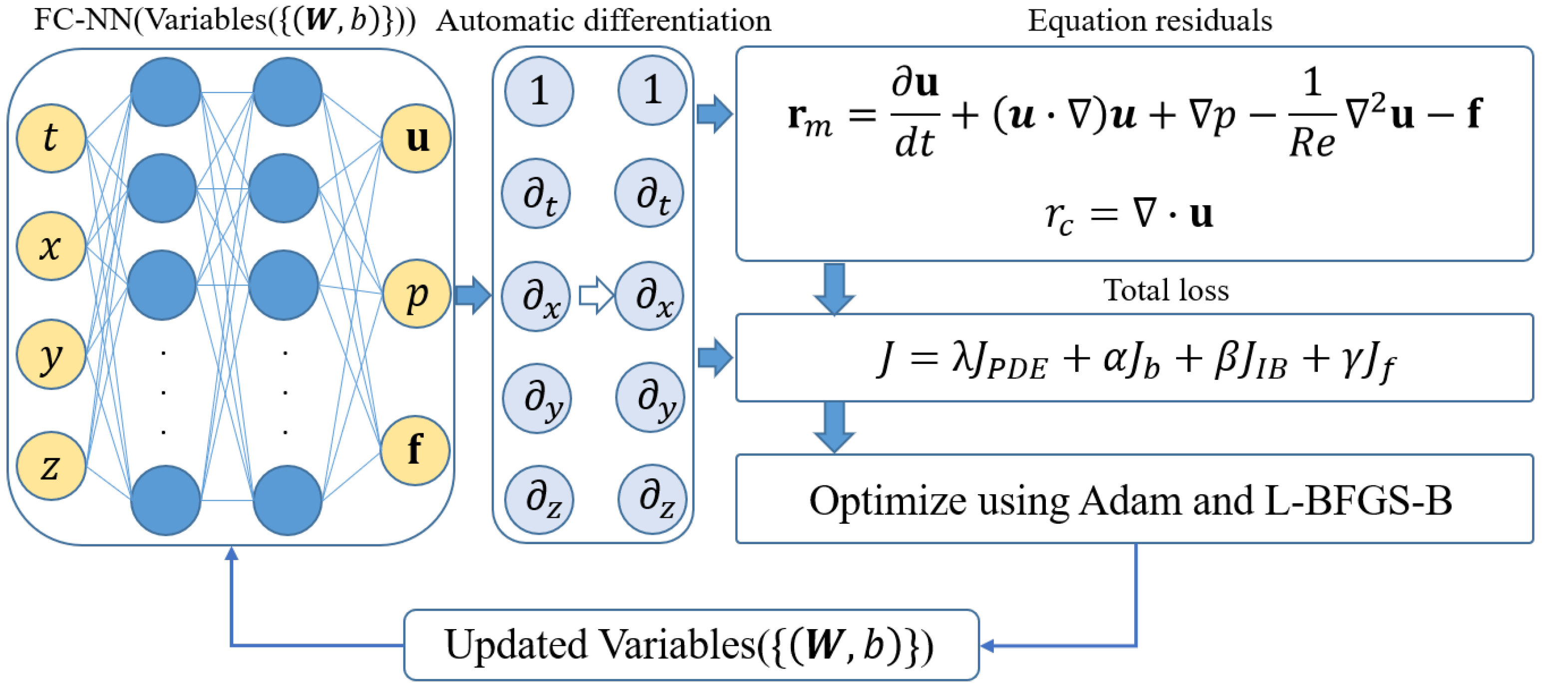
Figure 1.
A schematic diagram of the IB-PINN framework for solving an incompressible Navier–Stokes equation. The left part is the architecture of the DNN used in the simulation. The middle part illustrates the computation of derivatives by using automatic differentiation. The right part shows the formula for computing the loss function.

Figure 2.
A schematic diagram of the computational domain, the outer boundary and the locations of three sets of points required in computing the loss function of IB-PINN. The force penalties are imposed at the collocation points which are located inside the gray area. The distance from the inner boundary of the gray area to the immersed boundary is Δ.

Figure 3.
A schematic diagram of the computational domain and boundary conditions for the problem of flow over a circular cylinder placed in a channel.
Figure 3.
A schematic diagram of the computational domain and boundary conditions for the problem of flow over a circular cylinder placed in a channel.

Figure 4.
Convergence of loss function. The DNN of 6 × 100 is used. The number of collocation points is 72,365. The weights for the loss components are: λ = 1.0; α = 2.0; β = 2.0; γ = 1.0.
Figure 4.
Convergence of loss function. The DNN of 6 × 100 is used. The number of collocation points is 72,365. The weights for the loss components are: λ = 1.0; α = 2.0; β = 2.0; γ = 1.0.

Figure 5.
A comparison between the contours of velocity components obtained using Fluent, mesh-based IB and IB-PINN. (a) u-component (Fluent); (b) v-component (Fluent); (c) u-component (IB); (d) v-component (IB); (e) u-component (IB-PINN); (f) v-component (IB-PINN); (g) difference between IB-PINN and IB (u-component); (h) difference between IB-PINN and IB (v-component). In (g,h), the interior region is filled with white color, and the data are removed.

Figure 6.
The streamlines of the solutions obtained by using (a) Fluent, (b) mesh-based IB method and (c) IB-PINN.
Figure 6.
The streamlines of the solutions obtained by using (a) Fluent, (b) mesh-based IB method and (c) IB-PINN.

Figure 7.
A comparison between the velocity profiles obtained using Fluent, mesh-based IB and IB-PINN. (a) streamwise velocity profile along the horizontal centerline; (b) streamwise velocity profile along the vertical line passing through the center of the cylinder. The gray rectangles denote the segment inside the cylinder.

Figure 8.
A comparison between the pressure contours obtained by using Fluent and IB-PINN. (a) pressure (Fluent); (b) pressure (IB-PINN); (c) difference in pressure between IB-PINN and Fluent. For the solution of IB-PINN, the interior region is filled with white color and the data are removed.
Figure 8.
A comparison between the pressure contours obtained by using Fluent and IB-PINN. (a) pressure (Fluent); (b) pressure (IB-PINN); (c) difference in pressure between IB-PINN and Fluent. For the solution of IB-PINN, the interior region is filled with white color and the data are removed.

Figure 9.
A comparison between the distributions of the pressure coefficient along the cylinder surface obtained using Fluent and IB-PINN. The pressure coefficient is defined as , where .
Figure 9.
A comparison between the distributions of the pressure coefficient along the cylinder surface obtained using Fluent and IB-PINN. The pressure coefficient is defined as , where .

Figure 10.
Components of volume forces obtained by using IB-PINN and mesh-based IB method. (a) x-component (IB-PINN); (b) y-component (IB-PINN); (c) x-component (IB); (d) y-component (IB).
Figure 10.
Components of volume forces obtained by using IB-PINN and mesh-based IB method. (a) x-component (IB-PINN); (b) y-component (IB-PINN); (c) x-component (IB); (d) y-component (IB).

Figure 11.
Influence of the number of Adam iterations on convergence of training: (a) final loss as a function of the number of Adam iterations; (b) convergence histories of training for different numbers of Adam iterations.
Figure 11.
Influence of the number of Adam iterations on convergence of training: (a) final loss as a function of the number of Adam iterations; (b) convergence histories of training for different numbers of Adam iterations.

Figure 12.
Influences of the weights on final loss and prediction error: (a) variable λ with α = 2.0; β = 2.0; γ = 1.0; (b) variable α with λ = 1.0; β = 2.0; γ = 1.0; (c) variable β with λ = 1.0; α = 2.0; γ = 1.0; (d) variable γ with λ = 1.0; α = 2.0; β = 2.0.
Figure 12.
Influences of the weights on final loss and prediction error: (a) variable λ with α = 2.0; β = 2.0; γ = 1.0; (b) variable α with λ = 1.0; β = 2.0; γ = 1.0; (c) variable β with λ = 1.0; α = 2.0; γ = 1.0; (d) variable γ with λ = 1.0; α = 2.0; β = 2.0.

Figure 13.
Influences of the number of collocation points on (a) velocity error and (b) final loss.

Figure 14.
Influence of the number of marker points on velocity error. The dashed line denotes the place where the resolutions of marker points and collocation points are compatible.
Figure 14.
Influence of the number of marker points on velocity error. The dashed line denotes the place where the resolutions of marker points and collocation points are compatible.


Table 1.
The length and position of the separation bubble, the separation angle and the drag coefficient obtained using Ansys Fluent, mesh-based IB method and IB-PINN.
Table 1.
The length and position of the separation bubble, the separation angle and the drag coefficient obtained using Ansys Fluent, mesh-based IB method and IB-PINN.
| Fluent | 1.19 | 0.45 | 0.48 | 47.7° | 2.17 |
| IB | 1.19 | 0.46 | 0.48 | 46.7° | 2.21 |
| IB-PINN | 1.17 | 0.45 | 0.48 | 46.7° | 2.18 |
Table 2.
Final loss and velocity error obtained in nine DNNs with different configurations.
| 90 | 100 | 110 | ||
|---|---|---|---|---|
| 5 | Final Loss | 7.3764 × 10 | 8.1033 × 10 | 5.4935 × 10 |
| (%) | 0.28 | 0.27 | 0.26 | |
| (%) | 0.64 | 0.84 | 2.65 | |
| 6 | Final Loss | 5.8943 × 10 | 3.8017 × 10 | 4.4175 × 10 |
| (%) | 0.28 | 0.16 | 0.25 | |
| (%) | 0.87 | 0.62 | 0.82 | |
| 7 | Final Loss | 3.4572 × 10 | 4.1086 × 10 | 3.2451 × 10 |
| (%) | 0.20 | 0.22 | 0.20 | |
| (%) | 1.18 | 0.96 | 0.60 |
Table 3.
Final loss, velocity error and drag coefficient obtained in IB-PINNs with and without the interior force compactness constraint.
Table 3.
Final loss, velocity error and drag coefficient obtained in IB-PINNs with and without the interior force compactness constraint.
| Final Loss | (%) | (%) | ||
|---|---|---|---|---|
| With interior constraint | 2.5749 × 10 −3 | 3.10 | 6.77 | 1.96 |
| Without interior constraint | 3.8017 × 10 −5 | 0.16 | 0.62 | 2.21 |
Table 4.
A comparison of the performances in re-training the DNNs using original and transfer learning approaches.
Table 4.
A comparison of the performances in re-training the DNNs using original and transfer learning approaches.
| Original | Tranfer Learning | |||||||
|---|---|---|---|---|---|---|---|---|
| # Iterations | Final Loss | (%) | (%) | # Iterations | Final Loss | (%) | (%) | |
| Re = 10 | 45011 | 8.7173 × 10 −4 | 1.62 | 2.50 | 38258 | 2.7832 × 10 −4 | 0.79 | 1.36 |
| Re = 20 | 81341 | 2.1812 × 10 −4 | 0.47 | 1.23 | 25420 | 7.3278 × 10 −5 | 0.27 | 0.82 |
| Re = 30 | 53915 | 4.7878 × 10 −5 | 0.19 | 0.78 | 11500 | 5.6311 × 10 −5 | 0.24 | 0.78 |
Publisher’s Note: MDPI stays neutral with regard to jurisdictional claims in published maps and institutional affiliations. |
© 2022 by the authors. Licensee MDPI, Basel, Switzerland. This article is an open access article distributed under the terms and conditions of the Creative Commons Attribution (CC BY) license (https://creativecommons.org/licenses/by/4.0/).
Share and Cite
MDPI and ACS Style
Huang, Y.; Zhang, Z.; Zhang, X. A Direct-Forcing Immersed Boundary Method for Incompressible Flows Based on Physics-Informed Neural Network. Fluids 2022, 7, 56. https://0-doi-org.brum.beds.ac.uk/10.3390/fluids7020056
AMA Style
Huang Y, Zhang Z, Zhang X. A Direct-Forcing Immersed Boundary Method for Incompressible Flows Based on Physics-Informed Neural Network. Fluids. 2022; 7(2):56. https://0-doi-org.brum.beds.ac.uk/10.3390/fluids7020056
Chicago/Turabian StyleHuang, Yi, Zhiyu Zhang, and Xing Zhang. 2022. "A Direct-Forcing Immersed Boundary Method for Incompressible Flows Based on Physics-Informed Neural Network" Fluids 7, no. 2: 56. https://0-doi-org.brum.beds.ac.uk/10.3390/fluids7020056