
Adaptive Data-Driven Model Order Reduction for Unsteady Aerodynamics


Aerospace Centre, Department Mechanical and Aerospace Engineering, University of Strathclyde, 75 Montrose Street, Glasgow G1 1XJ, UK
*
Author to whom correspondence should be addressed.
Fluids 2022, 7(4), 130; https://0-doi-org.brum.beds.ac.uk/10.3390/fluids7040130
Submission received: 31 December 2021
/
Revised: 28 March 2022
/
Accepted: 29 March 2022
/
Published: 6 April 2022
(This article belongs to the Special Issue Reduced Order Models for Computational Fluid Dynamics)
Abstract
:A data-driven adaptive reduced order modelling approach is presented for the reconstruction of impulsively started and vortex-dominated flows. A residual-based error metric is presented for the first time in the framework of the adaptive approach. The residual-based adaptive Reduced Order Modelling selects locally in time the most accurate reduced model approach on the basis of the lowest residual produced by substituting the reconstructed flow field into a finite volume discretisation of the Navier–Stokes equations. A study of such an error metric was performed to assess the performance of the resulting residual-based adaptive framework with respect to a single-ROM approach based on the classical proper orthogonal decomposition, as the number of modes is varied. Two- and three-dimensional unsteady flows were considered to demonstrate the key features of the method and its performance.
1. Introduction
The development of algorithms capable of reducing the computational efforts required to obtain numerical solutions to aerodynamic problems has attracted much attention in the past decades [1,2,3,4]. The aim being to find the optimal trade-off between accuracy and cost, recent trends have seen the emergence of the so-called data-driven Reduced Order Models (ROMs) [5]. These are techniques where a set of reference data, called the training set, is collected and scrutinised to identify the relevant dynamics underlying the flow under investigation, which is subsequently used to make predictions for new untested conditions in a fast and accurate manner. Unsteady problems in fluid dynamics are good candidates for the application of reduced order modelling since time dynamics of high-dimensional fluid systems is likely to lie in a much lower dimensional space than the original high-dimensional system [6]. Nevertheless, highly nonlinear unsteady flows pose several challenges to model order reduction techniques as they can exhibit time-varying dominant and underlying features that might not always be easily identified. This is why much attention has been devoted recently to the formulation of ROM techniques specifically targeting unsteady flow physics [7,8,9].
A widely used algorithm to achieve order reduction is Proper Orthogonal Decomposition (POD) [10,11]. The algorithm extracts a set of orthogonal basis functions that identify an optimal low-dimensional linear manifold. The evolution of the system on this linear space can then be obtained by intrusively projecting the system governing equations onto the low-dimensional manifold [12,13,14] or alternatively using non-intrusive techniques that rely on interpolation [15,16,17] or machine learning algorithms [18,19,20,21]. The POD basis functions are orthogonal and optimal with respect to an energy norm, which means that they are the closest basis to the original dataset with respect to any other linear basis obtained adopting the same norm [22]. Nevertheless, POD has been recognised to have some limitations in extracting pure dynamics information [7,23], and alternatives have been proposed [8,9,24]. One of the drawbacks of POD is the energy criterion used to extract the basis functions. When the truncation of the initial set of modes is considered, only the most energetic flow primitives are retained. This might cause the loss of important spatial structures, which are low in energy, but important for the time dynamics [23]. Usually the neglected spatial structures are the ones associated with dissipation, and not considering them is likely to cause instabilities in time. To avoid inaccuracies related to the POD basis, ad hoc fixes have been introduced, which include adding damping terms [25] or performing calibration techniques to adjust the POD coefficients, in order to take into account the effect of the unresolved modes. Moreover, it can happen that the most energetic modes are not representative of physical coherent structures in the flow [9] and therefore not able to represent the actual dynamics in a low-dimensional space. When reconstructing certain classes of flows, variants of POD such as spectral POD [9] and diverse formulations of Dynamic Mode Decomposition (DMD) [8,24,26,27,28] have been found to perform better than POD. However, the exploration of these variants revealed that a unique, single-ROM approach cannot be identified that consistently outperforms other methods when used to reconstruct a flow whose characteristics are not known a priori, i.e., a flow for which it is not known if it is periodic, quasi-periodic, or shows some otherwise well-defined trend, etc.
In order to cope with this circumstance, a new strategy has been recently introduced that promotes synergy among different techniques for basis extraction [29]. The so-called adaptive ROM framework implements a strategy that automatically, at every instant of time, is capable of selecting locally a set of basis functions proven to provide the best accuracy possible in reconstructing the flow dynamics among a collection of methods available. The concept of adaptivity has been used in the recent literature on ROM [30,31,32], but it has not been developed in the sense of realising an adaptive choice of basis functions from different techniques. In all these existing examples, POD has always been the basis to elaborate the adaptivity in different manners. Moreover, in the wider field of surrogate modelling, there has been work performed where error metrics are used to choose the best-fitting model [33]. The originality in [29] stands therefore in combining different sets of basis functions in a unique framework, which aims at introducing a dynamic component that can balance the energy-only-based description provided by POD. Key to the adaptive ROM framework is the definition of a metric to judge what is the best method. In [29], the adaptive framework uses a direct error estimation, where a snapshot is excluded from the training set and used to compute the difference between that and a corresponding ROM solution. Other than not allowing exploiting all the available snapshots for training, such a direct approach bears a certain level of inaccuracy when evaluating the error at points for which a high-fidelity solution is not available. This means that the direct method, despite being an immediate natural choice, leaves the adaptive framework with a heterogeneous measure of the ROM reconstruction, likely to be accurate in the test points and more uncertain in other locations where some sort of interpolation or nearby error values are used.
In the present work, an a posteriori error measure is adopted for use in the framework of [29]. This metric uses the residual of the Navier–Stokes equations obtained by substituting the ROM solution into a finite volume discretisation. Using the residual does not require excluding snapshots from the initial set of training samples and, more importantly, promotes a more consistent estimate of the error for the whole parameter space. Since the error can be evaluated at many points at a low cost, estimates for all other points can be more accurately obtained by interpolation. This approach was first introduced in [34], while this work extends the analysis presented there. A sensitivity analysis is performed with respect to the number of modes used for reconstructions. How this affects the reconstruction is discussed with the aim of understanding how the residual-based error measure is able to provide improvements over a single-ROM approach. This element is key to assessing the ability of the adaptive framework to produce improved solutions with a lower number of degrees of freedom than a single-ROM approach. Since the aim of the framework is to perform effectively and efficiently over a wide class of unsteady flows, problems with different flow physics are considered here, e.g., flow with no specific periodic pattern or development and flow that starts with a highly nonlinear generation and interaction of vortices and then develops towards an advection–diffusion-dominated flow, among others.
A practical application of the framework is the enrichment of the nonlinear time dynamics of a problem. Provided that the physical processes are contained with sufficient detail in the snapshot set, the user can precisely identify in time–space where certain events occur, e.g., flow separation or vortex breakdown. This is made possible since the constraint on the time step size (due to increasing computational complexity) is eliminated by the framework. Similarly, the framework can be leveraged with the intent of saving storage space. The user can save CFD solutions only at some of the time steps to construct the training set. Then, solutions at any of the intermediate time steps can be recovered in a fast manner, e.g., in comparison to direct interpolation on the full-order model.
The paper is structured as follows: Section 2 describes the mathematical formulation of the adaptive ROM problem based on the residual error metric; Section 3 presents the implementation of the adaptive framework, describing also the set of ROMs considered; Section 4 presents the numerical derivation of the residual error measure used in the adaptive framework; Section 5 proposes a sensitivity analysis on the residual with respect to the number of modes retained in the adaptive framework presenting two demonstration cases, namely the impulsive start of a NACA0009 airfoil and a 30P30N airfoil; Section 6 presents a 3D test case, where an analysis of the unsteady vortex dynamics past a delta wing are provided, including the analysis of vortex breakdown over the wing; then, in Section 7 an application of the adaptive framework is provided in the context of three delta wings in a formation flight; finally, Section 8 presents final remarks and the outlook.
2. Mathematical Formulation of the Adaptive ROM Framework for Multi-Query Problems
Let be a set of solutions to the Navier–Stokes equations, over a given tessellation of the physical domain , where , represents the space of all possible solutions, and represents the number of degrees of freedom of the problem, depending on the specific tessellation used. A continuous definition of the residual associated with these solutions, for the specific case of unsteady problems, is defined as:
where w is a function with compact support, according to the finite volume formulation, represents the vector of conservative variables, and , are the vectors of convective and viscous fluxes, respectively,
In Equation (2), is the flow density, is the velocity vector, P is the thermodynamic pressure, is the total energy, is the viscous stress tensor, and is the heat flux vector.
Let be a set of low-dimensional solutions computed from different ROM algorithms at an instance of the many-query problem considered, which can be different from the set of times used to train the ROM, i.e., the set S. N represents the number of degrees of freedom of the set of low-dimensional solutions, which is often much smaller than the number of degrees of freedom of the original problem (). The rationale at the basis of the proposed adaptive framework is to select the low-dimensional solution that is closest to the solution directly computed in . In this work, a residual-based approach is introduced to assess the various ROM solutions, which consists of the evaluation of the residual defined in Equation (1). Hence, the adaptive framework aims at selecting the reduced order method that satisfies the following condition:
where denotes the Euclidean norm. The adaptive framework selects the low-dimensional solution that generates the minimum residual when substituted in the set of Navier–Stokes equations.
3. Implementation of Adaptive ROM
In terms of practical steps, the adaptive framework can be schematised as follows, separated into an offline and online phase. The offline phase consists of three steps:
- (1)
- Generation of the dataset , where indicates the entire set of conservative variables;
- (2)
- Construction of R low-dimensional models, where R is defined by the user on the basis of the ROM algorithms available, and computation of their reconstruction on a specified time grid, , with the specified time grid;
- (3)
- Error estimation for each method on the specified time grid through the residual . Each method will have, at each time instance of the time grid used, a set of residuals corresponding to the set of conservative variables of the problem at hand.
There is no limitation in the number and type of ROMs to include in the adaptive framework, and methods can be added and removed at any time, also on the basis of the specific problem at hand. Consequently, at the end of the offline phase, a certain number of different basis sets are extracted and a residual database is obtained associated with each ROM. A residual database is constructed by feeding ROM solutions to the same solver that was used to obtain high-fidelity snapshots for the training set. The specific solver used in the present work is the open-source CFD solver SU2 [35]. The online phase consists of two very fast steps:
- (1)
- Using as inputs the residual database and the desired time instant of the many-query problem, selecting the best low-dimensional model for each conservative variable in ;
- (2)
- Computing the reconstruction for each conservative variable in , using a formula based on the method selected.
A schematic of the complete offline-online procedure is reported in Algorithm 1. Since the error definition used in the adaptive strategy is equation based, i.e., it uses the original set of governing equations of the system, the adaptive framework implemented will be also referred to as residual-based adaptive ROM. Moreover, considering the definition of the residual error, it will always be assumed hereafter that the adaptive framework is applied to the entire set of conservative variables, namely the vector in Equation (2), which are all treated as independent variables to build the low-dimensional space.
| Algorithm 1: Adaptive reduced order modelling framework. |
 |
Basis Identification and Flow Reconstruction
Three model order reduction algorithms are considered for building the adaptive framework in this work, namely POD, DMD, and Recursive Dynamic Mode Decomposition (RDMD). The last two algorithms are introduced in an effort to better exploit the time correlation among snapshots, which is not explicitly considered by POD. All three algorithms are based on the following assumption for expressing the approximated ROM solution:
where is the number of modes and is the approximated ROM solution of conserved quantities, which is expressed as a linear combination of spatial basis functions through time dynamics coefficients . The assumption in Equation (4) makes these methods linear, even though nonlinearities in space and time can be resolved through nonlinear temporal and spatial eigenfunctions, and , respectively. In the present work, both spatial and temporal eigenfunctions are extracted through data. The POD spatial eigenfunctions are extracted using the method of snapshots introduced by Sirovich [36], and the DMD spatial eigenfunctions are obtained using the exact DMD algorithm described in [37], whereas the RDMD spatial modes are computed through the algorithm introduced in [24]. The coefficients in the case of the DMD method are computed as follows:
where and are constant values extracted from the data. is the th DMD eigenvalue computed according to the exact DMD algorithm [37]; are instead computed according to [38]. POD and RDMD provide instead discretised temporal eigenvectors, the temporal eigenfunctions, which are later interpolated using Radial Basis Function (RBF) interpolation to obtain a continuous function of time:
where is a polynomial of low degree and the basis function f is a real-valued function [39], which in the present work was chosen to be a Gaussian. The are referred to as the centres of the RBF, and they are the time instants corresponding to the training snapshots. On the basis of these formulas, the online phase of the adaptive framework is completely non-intrusive. An important note in relation to reconstructions computed using the adaptive selection is that at present, time continuity is not enforced when solutions at subsequent time instants are obtained using different ROM methods.
4. Residual-Based Error Estimation
A derivation of the residual error introduced in Section 2 is reported in the current section. A finite volume discretisation of the initial set of Navier–Stokes Equation is considered, and the residual error is then computed by substituting an approximated ROM solution provided by Equation (4) into such a discretisation. Since the focus is on unsteady fluid problems, an edge-based finite volume formulation is considered for the residual error, equipped with a Backward Difference Formula (BDF) for the unsteady term, which ensures second-order accuracy. The formula is derived in the following. The Navier–Stokes equations in conservative form reads:
where indicates the vector of conservative variables and represents the vector of convective and viscous fluxes, whose analytical expressions are reported in Equation (2). Considering a finite volume approach, Equation (7) is integrated over the generic cell of the computational domain, obtaining:
where the second integral is obtained by applying the divergence theorem. Equation (8) is still exact, and approximations are introduced to compute the volume and surface integrals. Specifically, a linear variation of the quantity is considered over the generic cell , and the generic flux is evaluated over the edges of cell considering an intermediate state , which is computed on the basis of the value of in the actual cell and the one in the neighbour cell sharing the same edge. The following approximations are therefore introduced:
where is the flux computed at the intermediate state and , with the area of the generic edge. Substituting in Equation (8) and defining as the residual produced by the approximations introduced,
A second-order BDF is finally considered for the temporal derivative, obtaining the final expression of the residual for the generic cell and for the entire set of the conservative variables,
where and represents the additional contribution to the residual coming from the discretisation of the temporal derivative. represents the number of points of the computational domain. The residual is evaluated at time instant . To obtain a final measure of the residual error, the norm of over the entire computational domain is computed, normalised by the number of points. Therefore, for each conservative variable:
with the residual produced by the th conservative variable, in the th cell, according to Equation (12). The in Equation (12) represents an additional parameter for this particular error definition and dictates at which time instants the ROM reconstructions are computed to evaluate the residual. This can be different from the time step used for the unsteady CFD simulation, denoted hereafter as . In Step 3 of the offline phase, is used for the computation of the error database (see Section 3). Another important parameter used in this work is , which is the time step used for the sampling of the training snapshots to build the adaptive ROM.
5. Sensitivity with Respect to the Number of Modes
In order to investigate the capabilities of the adaptive framework as the number of modes retained is varied, an integral of the residual error with respect to time is presented as a function of the number of modes:
where is the time interval used to train each ROM and is the residual error defined in Equation (13) for a generic conservative variable. To compute the integral, the residual error is computed on a set of test points equispaced in time and with a resolution , which represents the same procedure adopted to build the residual error database for the adaptive ROM. The integral is then approximated using a trapezoidal rule. An additional quantity will be reported, which provides a better understanding of the improvements introduced by the adaptive framework locally in time, varying the number of modes. This quantity represents the difference of the residual error produced by the adaptive ROM and that produced by a single ROM,
where the subscripts A and S stand for adaptive and single, respectively, while still represents the residual error as defined in Equation (13), for a generic conservative variable. The expression single ROM refers to any ROM that extracts one set of global basis functions from the original set of snapshots. In the following analysis, is considered as the residual error of the POD method. This is because POD has been the most widely used method in the literature for implementing ROMs in the case of unsteady problems and it represents a good reference point for the community, even if the can represent the error of any single ROM. For the same reason, the analysis reported on for the adaptive framework will be compared with the POD technique as well. It is worth noting that, since the POD is also included in the adaptive ROM, the quantity defined in Equation (15) will always be a non-negative quantity.
5.1. Impulsive Start of a NACA0009 Airfoil
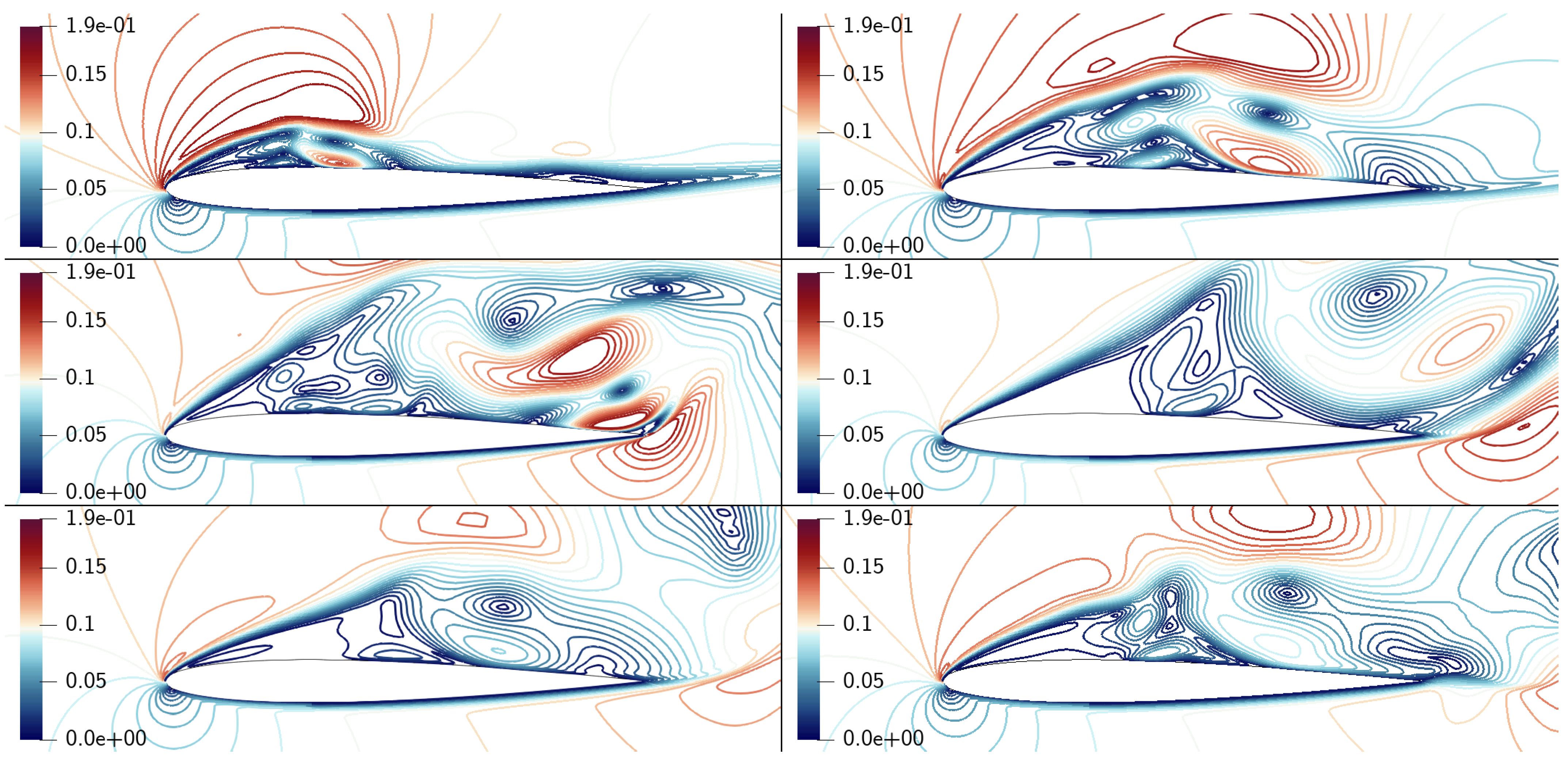
The impulsive start of a NACA0009 airfoil is considered here. The fixed freestream values and parameters used for the unsteady simulation are summarised in Table 1. Under these conditions, a vortex-dominated flow is established. In particular, the flow field is characterised by an initial laminar bubble that grows gradually in time until it interacts with the separated region near the trailing edge. This eventually leads to the onset of an instability in the airfoil wake, causing the development of a quasi-periodic vortex-shedding-like motion. The flow field is shown at different instants of time in Figure 1.
The mesh used for the domain discretisation is a viscous structured mesh with 91,039 elements and 91,650 grid points. The time discretisation is obtained using a constant time step, s, for advancing the unsteady simulation. As per the numerical setup for the high-fidelity simulation, the laminar Navier–Stokes equations were solved, using a second-order finite volume discretisation for the fluxes, adopting the standard MUSCL approach and a second-order dual-time stepping scheme to deal with the unsteady part for this and subsequent test cases. Note that with dual-time stepping, the CFL number only impacts the solution in pseudo-time. The convective fluxes were discretised using the Roe scheme. As the initial condition, the entire domain was initialised to freestream quantities, while the boundary conditions on the body and at the domain borders were no-slip (for momentum equations), adiabatic (for energy equation), and freestream quantities, respectively.
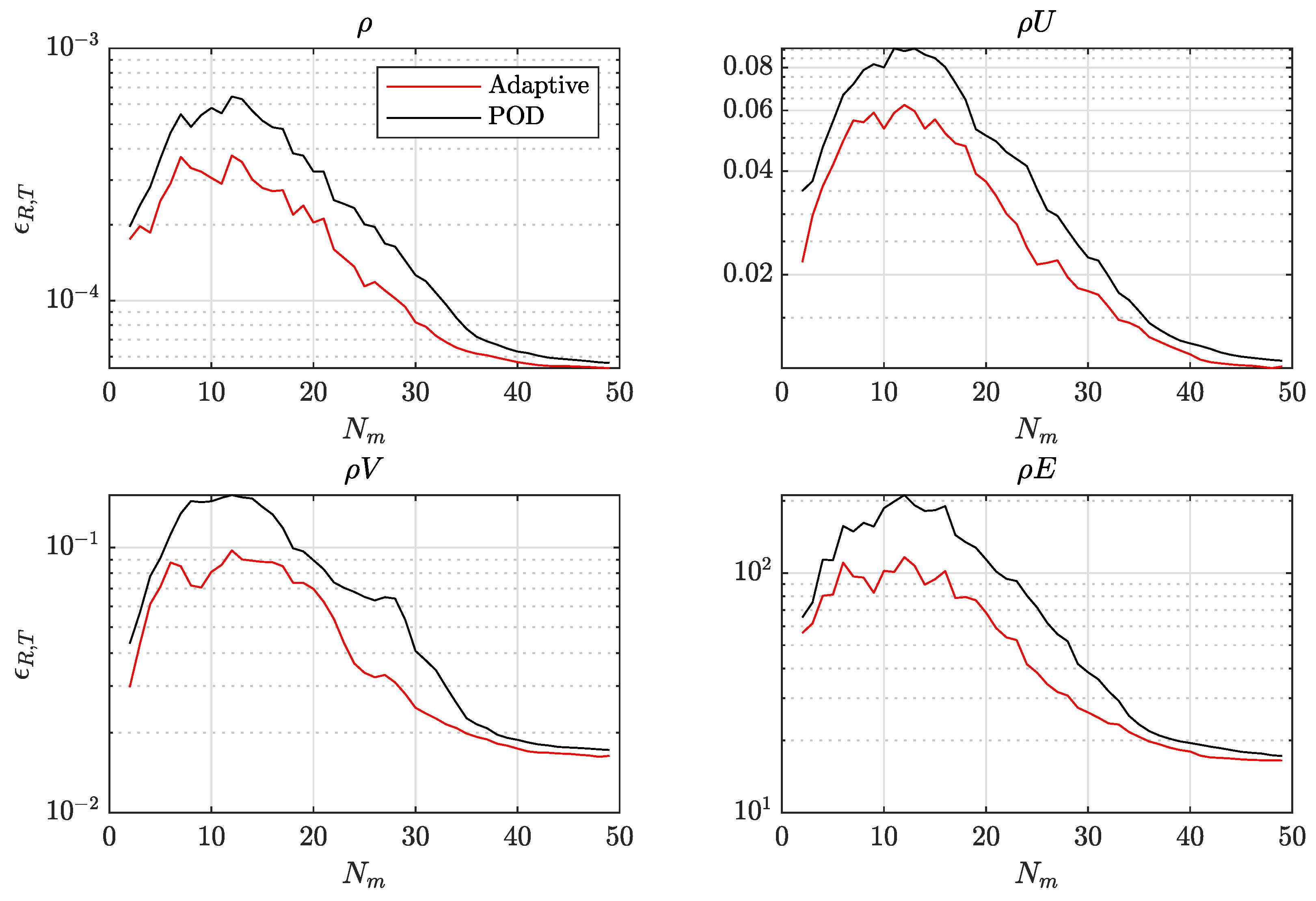
For the analysis of and , ROMs were constructed within the time window s, where the dynamics of interest take place, using a sampling of s, which results in a number of snapshots equally spaced in time. The maximum number of modes that can be used in the adaptive ROM is therefore 75. Figure 2 reports the quantity for the adaptive ROM and POD-only ROM, for the entire set of conservative variables. An interesting aspect to discuss for these plots is the presence of a nonmonotonic trend as the number of modes is increased. Indeed, the residual integral starts from relatively lower values when using very few modes and increases as other modes are added. Starting from a certain number of modes, the overall trend is then decreasing, reaching a minimum when the entire set of modes is used. The nonmonotonic behaviour can be linked to a physical interpretation of the modes. It is expected that the most important modes should carry information about large spatial structures, while higher modes solve for smaller spatial structures. When using very few modes, small spatial structures are not resolved and something closer to the mean field with little variation in time is reconstructed, which might be responsible for the lower residual. It is worth highlighting at this point that Equation (12) represents a weak discretisation of the set of initial governing equations of the system (the space of possible solutions is therefore expanded), and moreover, it is completely blind to the actual physical time considered. As more modes are added, new spatial structures start to be resolved, albeit with very low resolution, which causes the residual integral to increase. Once the number of modes is reached where all the spatial structures are present in the reconstructed flow field, adding additional modes will decrease the integral residual, since also small structures start to be resolved more accurately.
An illustration of this discussion can be seen in Figure 3, where a reconstruction at a specific time instant, provided by the adaptive ROM, is reported using two different numbers of modes that show the same residual integral from Figure 2, specifically 2 modes (on the left) and 28 modes (on the right). The reconstruction in the wake of the airfoil with two modes shows only averaged flow features, where the region of separated flow is clearly visible, but no structures in the wake are resolved. Moving to 28 modes, it can be noticed how more structures in the wake are resolved, but also new oscillations not present in the reference field are added. These oscillations will vanish only when more modes are added, with a consequent reduction of the residual error. The trend of with the number of modes is not a unique feature of the residual-based adaptive ROM used in the present work. As a matter of fact, considering the number of modes in the same way as the degrees of freedom of the computational mesh, the nonmonotonic behaviour has been observed also for the case of error estimators used for a steady linear advection–diffusion equation [40]. In particular, the authors in [40] define error estimators that show a nonmonotonic behaviour while increasing the size of the initial computational mesh.
Another important result from Figure 2 is that the improvement of the adaptive ROM over using the POD-only single ROM is higher when far fewer modes are used than the entire set of modes available (10–15 out of 75, on the basis of the distance between the red and black curves reported in Figure 2). Overall, the adaptive framework always performs better than pure POD in terms of residual integrals. Figure 4 shows , in log scale, in the box . White spaces correspond to , which means that POD has been chosen from the adaptive framework for that combination of time and number of modes. From the contours also, it is visible how the adaptive framework introduces improvements with respect to the Single ROM () when using a subset of all the modes available. As the number of modes is increased, the improvements introduced by the adaptive framework with respect to POD are less and less visible. This is obviously linked to the enrichment of the POD basis with the whole information content coming from the training snapshots, which is eventually able to reconstruct the entire dynamics contained in them.
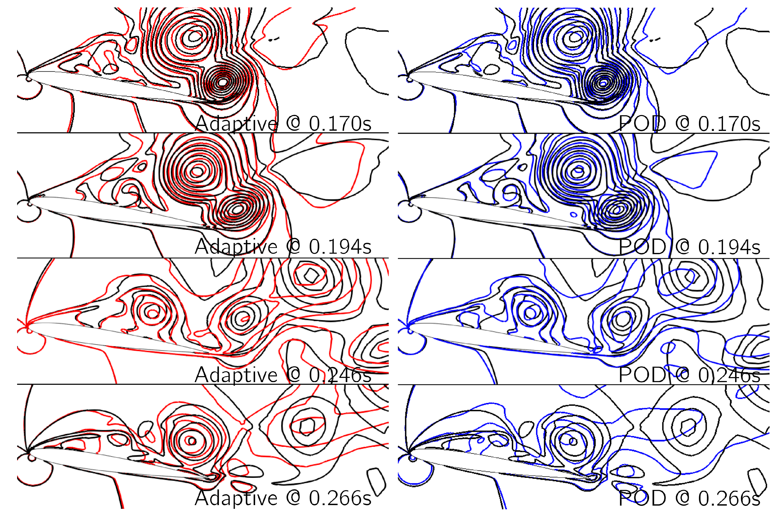
An adaptive ROM is finally built retaining only 10 modes out of the 75 available and used to compute a number of reconstructions of the entire flow field. These solutions are compared against the CFD reference solution and to reconstructions obtained using POD. In particular, Figure 5 shows the conservative variable density reconstructed at four different instants of time, where the first column presents the adaptive reconstruction and the second column reports the POD reconstruction, both compared against the reference solution. Even if some resolution is lost in capturing all spatial structures due to the selection of only a small subset of modes, it can be observed that the adaptive framework is able to provide a more accurate description than purely POD. This is especially apparent for the structures forming downstream, in the top right corner of the visualised flow field in Figure 5.
5.2. Impulsive Start of a 30P30N Multi-Element Airfoil
The 30P30N test case is now considered. The parameters used for the unsteady simulation are summarised in Table 2. The mesh used for the domain discretisation is a viscous hybrid mesh with 559,652 elements and 327,733 grid points. The flow field is shown in Figure 6.
The ROMs are built within the time window s where the dynamics of interest take place, using a sampling of s, which yields snapshots equispaced in time. Similar to the previous test case, Figure 7 reports the quantity for both adaptive and POD-only ROM and for the primary conservative variables. Since high-fidelity solutions for 30P30N are computed using RANS, modelling turbulence with SST, the turbulent variables were considered in the computation of the residual error for the primary variables, but they are not reported in the analysis. In Figure 7, a nonmonotonic behaviour of the residual integral can be observed with respect to the number of modes, and a similar discussion can be given as what was presented in Section 5.1.
Figure 8 shows the reconstruction of the density field obtained with the adaptive framework at a specific instant of time, for two sets of modes that present the same value of . Specifically, 6 modes were used for the reconstruction on the left and 17 modes for the one on the right. The black contour lines represent the reference CFD solution, and the reconstructed solution obtained using the adaptive framework is represented by red lines. Using only six modes, the details of the vortices detaching from the multiple airfoil surfaces, namely slat, main component and flap, are not captured at all, since these vortices are represented as a single large spatial structure. With 17 modes, more details of the detaching vortices can be observed, however still not merged. Moreover, additional oscillations in space are introduced, which vanish only with the addition of more modes. This balance between resolving only for large spatial structures (six-mode case) and resolving also for smaller structures, but introducing spatial oscillations in other regions of the flow field (17-mode case) explains the nonmonotonic behaviour in Figure 7. Another important aspect to consider is the advective nature of the problem, since the most important dynamics are linked to the advection of the vortices detaching from the various lifting surfaces. The spatial oscillations downstream of the starting vortices, visible on the right contours in Figure 8, are indeed not linked to the low resolution of spatial structures actually present in the flow field at that specific time instant; instead, they are caused by the advection of the starting vortices, which are transported to those regions in subsequent time instants. These oscillations vanish when adding higher-order modes. Figure 9 shows the quantity , in log scale, in the box . As for the previous test case, no common pattern can be identified in switching from one ROM to another over various instants of time and number of modes used; therefore, details on that are not reported. From the contours shown in Figure 9, it is apparent that the advantage of using the adaptive framework () is more significant when using a small subset of modes, and as the number of modes is increased, the improvement of the adaptive ROM over the single ROM gradually diminishes. This trend can also be observed in Figure 7 by comparing the integrals of the residuals. This is in agreement with the observations made for the NACA test case, and an equivalent explanation can be provided here.
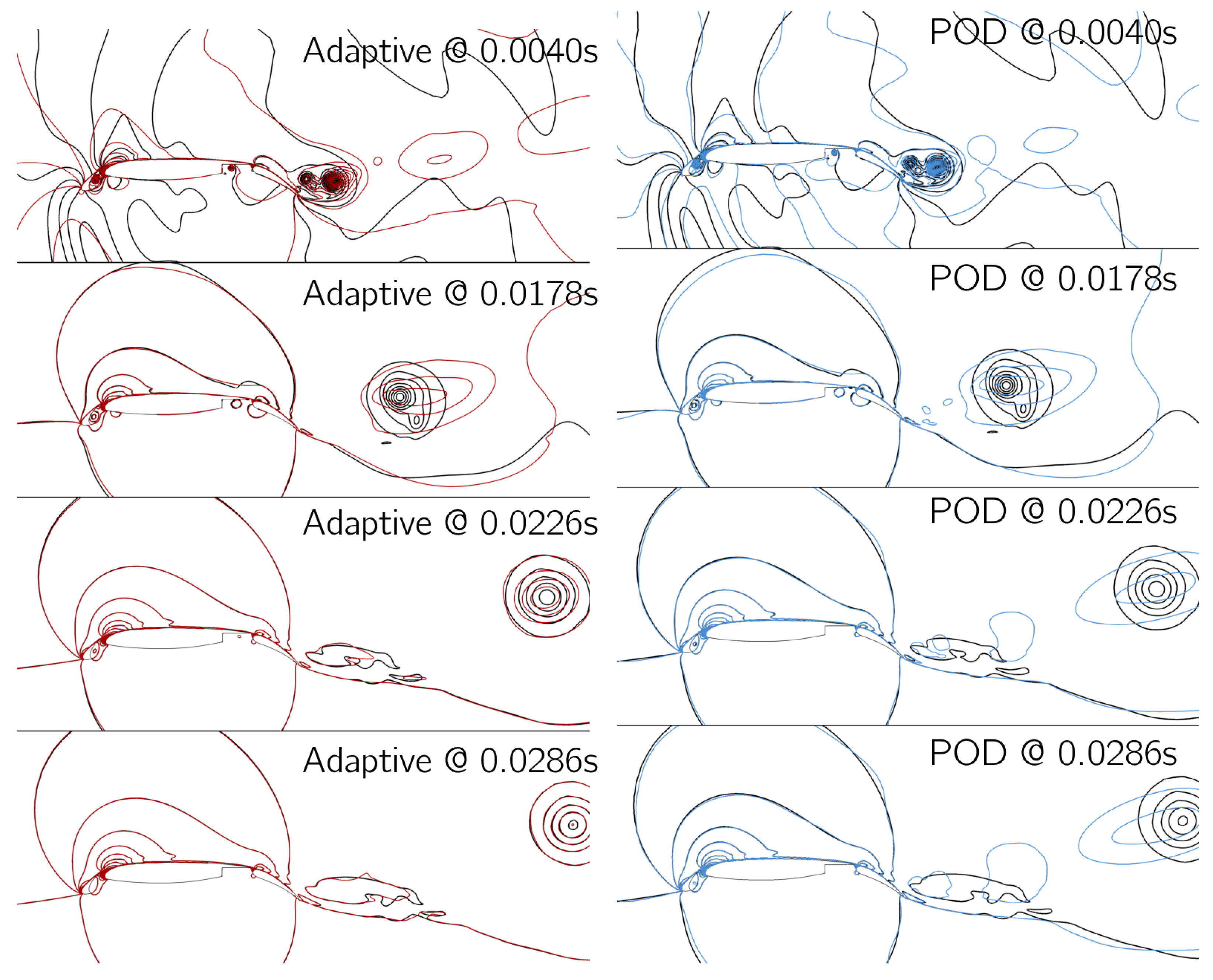
To compare their performance, adaptive and POD-only ROMs were built both retaining only 10 modes out of the 50 available, and a number of reconstructions were computed to show the improvements of the adaptive ROM over POD. Figure 10 shows the conservative variable density field for four instants of time, comparing the adaptive ROM and POD reconstructions to a reference CFD solution. In the very initial time window, some spurious oscillations are present for both methods (first row in Figure 10), as a consequence of using only a small subset of modes to describe the very strong initial transient. The second row in Figure 10 still shows poor accuracy in resolving the starting vortex for both techniques, but an overall improvement is observed using the adaptive ROM over pure POD. Finally, for the last two instants represented (last two rows in Figure 10), the starting vortex is more accurately resolved while propagating downstream with respect to a pure POD, which instead reconstructs the structure highly stretched in the streamwise direction and loses accuracy in resolution. The reconstruction with adaptive ROM also shows improvement near the airfoil surfaces when compared to POD.
6. Unsteady Dynamics of Vortices Past a Delta Wing
The flow past a delta wing configuration is now considered. The geometry and the freestream flow conditions were taken from the literature [41] with the only difference being the exclusion of the model sting present in the original configuration. The parameters used for the unsteady simulation are summarised in Table 3.
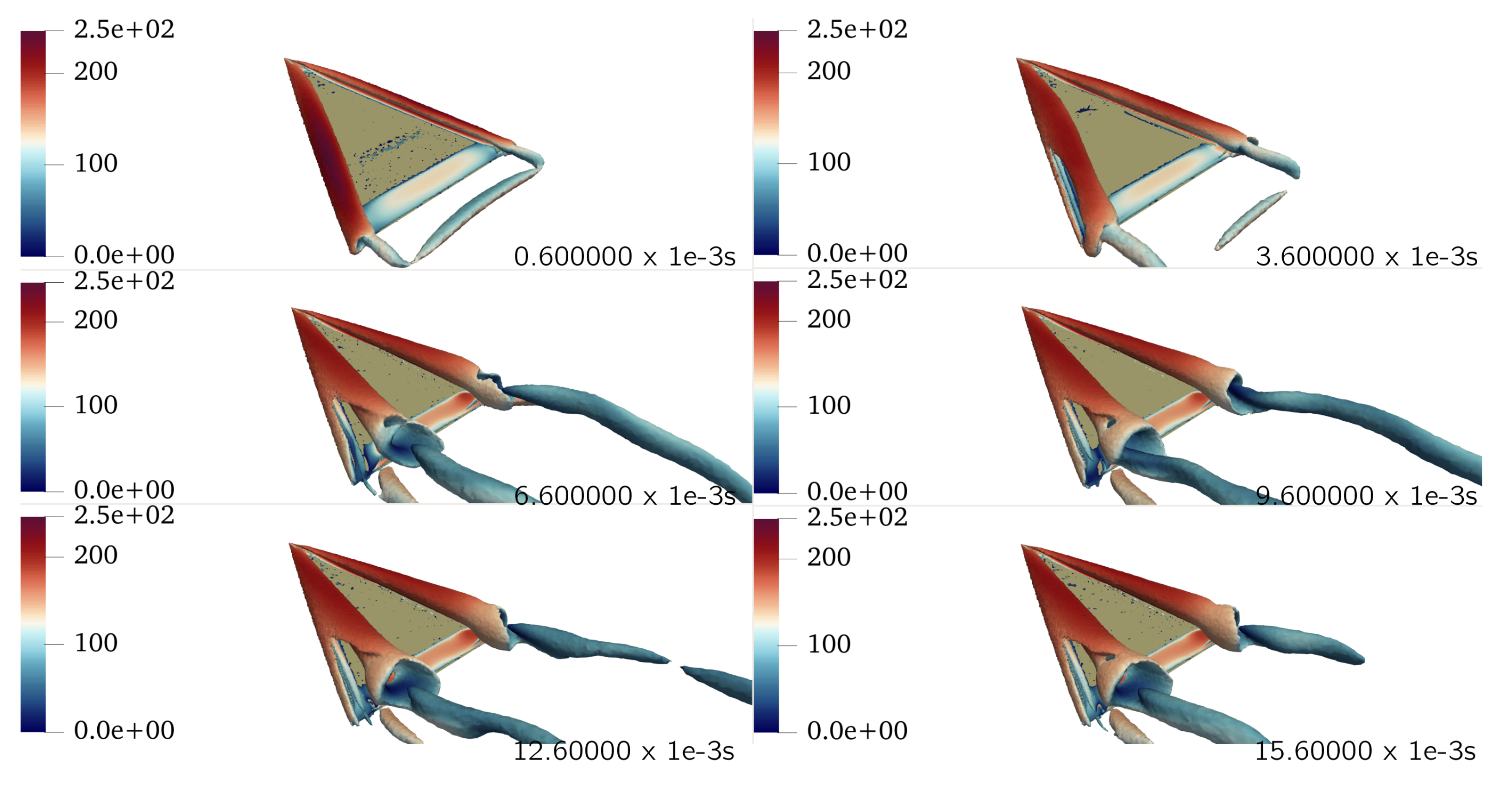
A hybrid mesh with 10,834,270 elements and 2,319,893 grid points was considered. A constant time step of s was used. The Reynolds-averaged Navier–Stokes equations were solved with a SST turbulence model, using a second-order finite volume discretisation for the fluxes (MUSCL approach) and a second-order dual-time stepping scheme to deal with the unsteady part. With the specific setup used, a quasi-periodic behaviour was eventually established that showed a vortex breakdown phenomenon [42,43]. Figure 11 illustrates a few snapshots where the vortical structures originating from the leading edge are represented by means of the Q-criterion. The reduced model was built over the time window s, during which the formation of the characteristic leading edge vortices and their breakdown in proximity of the trailing edge were observed. A sampling of s was used, which resulted in snapshots equally spaced in time. The time required for the database generation was approximately 10,500 core hours, with a maximum of 1000 iterations for the dual-time stepping scheme.
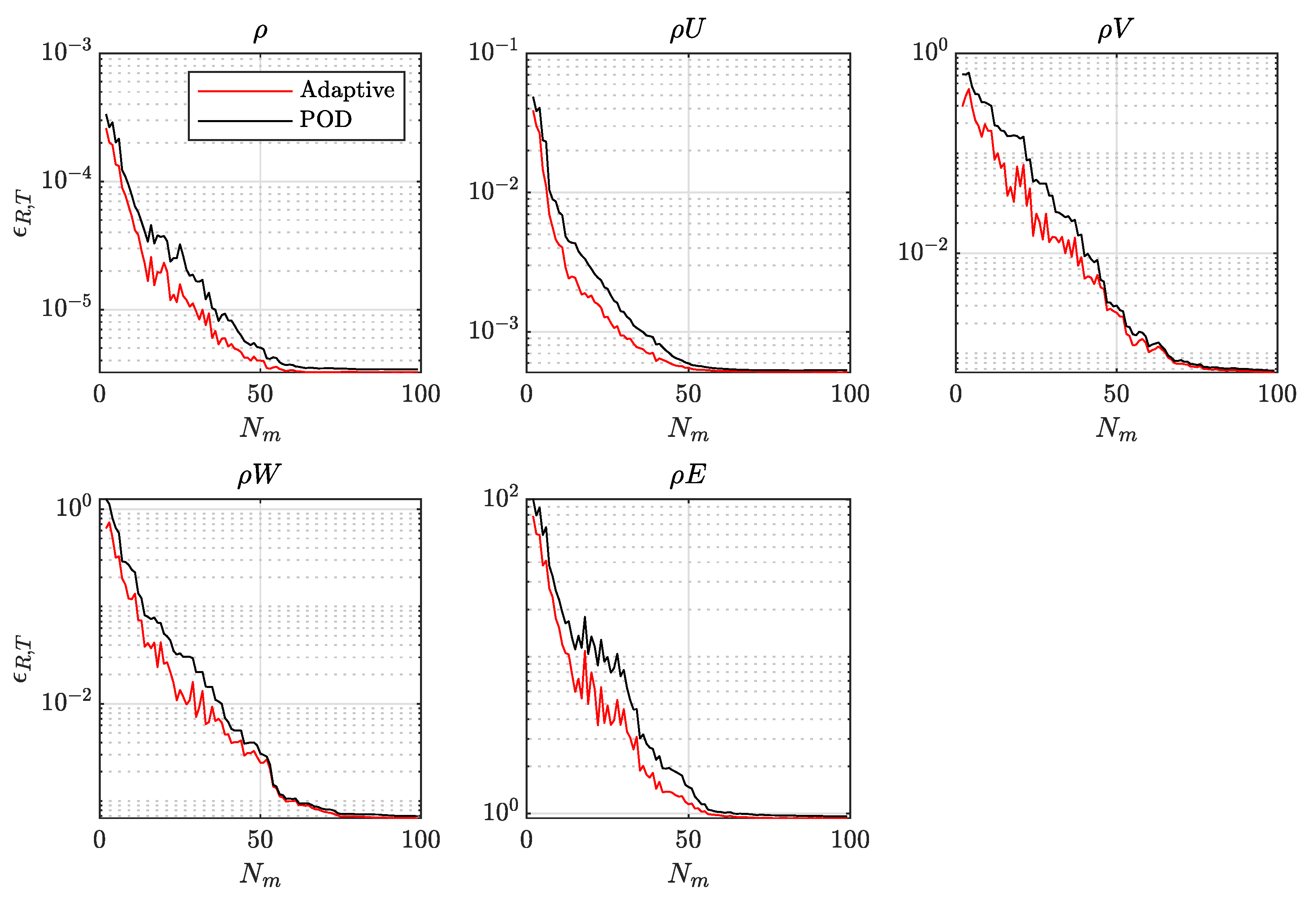
Figure 12 reports for the adaptive ROM and the reference POD for the conservative variables. It can be observed how the adaptive framework performs better overall than the single POD for all the set of conservative variables. From the contours of reported in Figure 13, it is evident how the adaptive framework introduces substantial improvements with respect to a single POD approach in terms of residual error, especially when using very few modes. High values of are in the region of a small number of modes, where the adaptive framework shows superior performance for almost the entire time window and especially in the second half, where the quasi-periodic vortex breakdown is established. This can be linked to the ability of the RDMD basis in describing the dynamics of attractors better than a POD basis [24]. Similar accuracy between the adaptive framework and single POD was observed while increasing the number of modes. In fact, adding more modes to the POD basis implies accounting for less energetic structures, resulting in an overall level of accuracy that is comparable to the adaptive framework.
In terms of a global measure such as , the superiority of the adaptive framework with respect to a single ROM might not be fully appreciated. However, when it comes to the ability to resolve local flow features and flow dynamics using very few modes, the adaptive framework leads to substantial improvements as illustrated in the following sections. To carry out this analysis, 10 out of 70 modes were considered. With this specific setting, the time required for the extraction of the set of features for the adaptive framework and the computation of the residual database was approximately 18 h (most of the time was required to extract the RDMD basis), while the extraction of the POD basis required less than one minute (no residual database required), both on a single core. The time required for one residual evaluation to generate the residual database is 700 s on a single core, as opposed to the 50 core hours required to compute one additional CFD solution. Finally, the online phase required only a few seconds to reconstruct the ROM solution at each desired time for both the adaptive framework and pure POD.
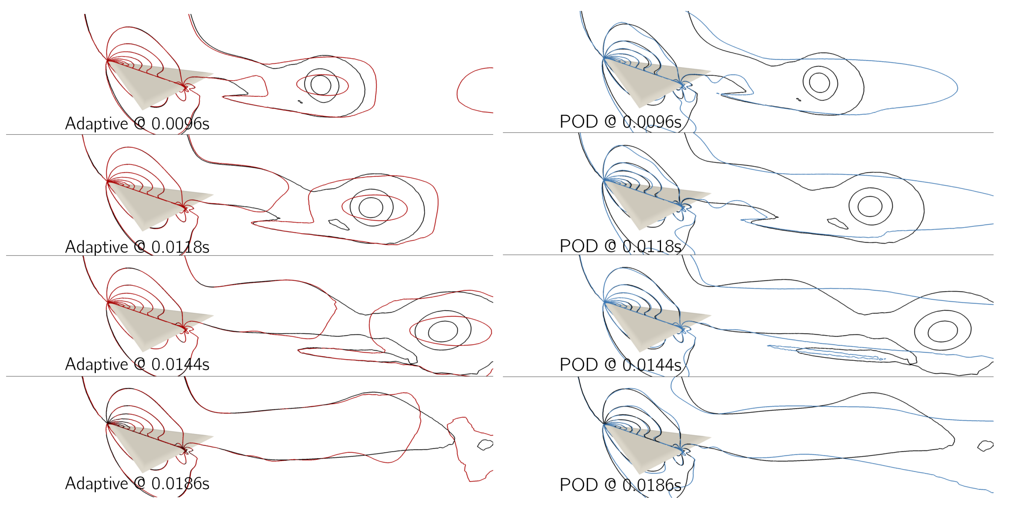
A comparison between the adaptive framework and the single POD was made with respect to the accuracy in reconstructing the entire flow field around the delta wing. Figure 14 reports the residual evaluation for the three methods in the adaptive framework (left column) and the choice of these methods over the investigated time window (bar plot on the right column). For the specific case of the main component of momentum and the two conservative variables and , RDMD performed better in the description of an attractor that is now quasi-periodic, namely the occurrence of the vortex breakdown once the initial transient due to the impulsive start vanishes. The observed oscillations at the border, usually appearing for the RDMD, are a consequence of the varying dynamics of the modes, associated with the quasi-periodic dynamics dictated by the vortex breakdown. The better performance of the adaptive framework is clearly visible in terms of reconstruction of the entire flow field in Figure 15, where a slice on the symmetry plane is reported and contours of the adaptive and POD techniques are compared against the contours of the reference CFD solution, for the density and for different instants of time. It can be noticed from this figure how the details of the trailing edge vortex transported downstream are completely lost with the POD reconstruction, while they are captured by the adaptive technique.
Analysis of the Vortex Breakdown over a Delta Wing
The capabilities of the adaptive ROM were assessed in terms of the ability to address the vortex breakdown mechanism. A different time window was now considered to build the adaptive ROM, which was s, and the initial time instant of the interval corresponded to a flow field where the leading edge vortices are almost fully developed and a clear breakdown station can be identified. In this time window, equally spaced in time snapshots were considered, which corresponds to a sampling frequency of s. There were 300 ROM solutions computed within the time window considered to enrich the description of the dynamics, as opposed to the 36 CFD solutions available within the same time window.
The criterion for the identification of the x coordinate of the breakdown point goes through three steps:
- (1)
- Computation of the velocity vector from the reconstructed conserved quantities;
- (2)
- Extraction of vortex core lines from the velocity volume solution;
- (3)
- Identification of the streamwise coordinate where the vortex core line associated with the main leading edge vortex is interrupted.
The interruption of the main vortex core line was assumed to be the point of breakdown onset of the leading edge vortex. The vortex cores tool available in Paraview 5.9.0 was used. The tool extracts vortex cores using the parallel vectors method [44,45], applied to the velocity vector field. According to the literature [46], a reduced velocity is defined that represents the actual flow field velocity minus its component in the direction of the real eigenvector of its Jacobian (only regions with complex eigenvalues are considered). Points where is zero are identified as points belonging to a vortex core line. The following eigenvalue problem was solved,
and points were searched that satisfy the equation for the real eigenvalue .
Figure 16 reports the delta wing 3D view with the vortex core lines associated with the two main leading edge vortices. It can be noted how the vortex lines have a spatial behaviour that is almost linear until a specific streamwise station of the delta wing. After that, the abrupt change in the vortices’ structures linked to the breakdown onset interrupts the lines. This might be linked to the specific resolution of the mesh used for the present study to describe the complex irregular structure of the earlier stages of the vortex breakdown, which resorts to a more organised spiralling motion at the station further downstream of the delta wing. Nevertheless, the interruption of the line can still be used as an indicator for the point of vortex breakdown onset, as it is still related to abrupt changes in the characteristics of the vortex. This also clarifies the definition of the coordinate of breakdown that will be used for the analysis below.
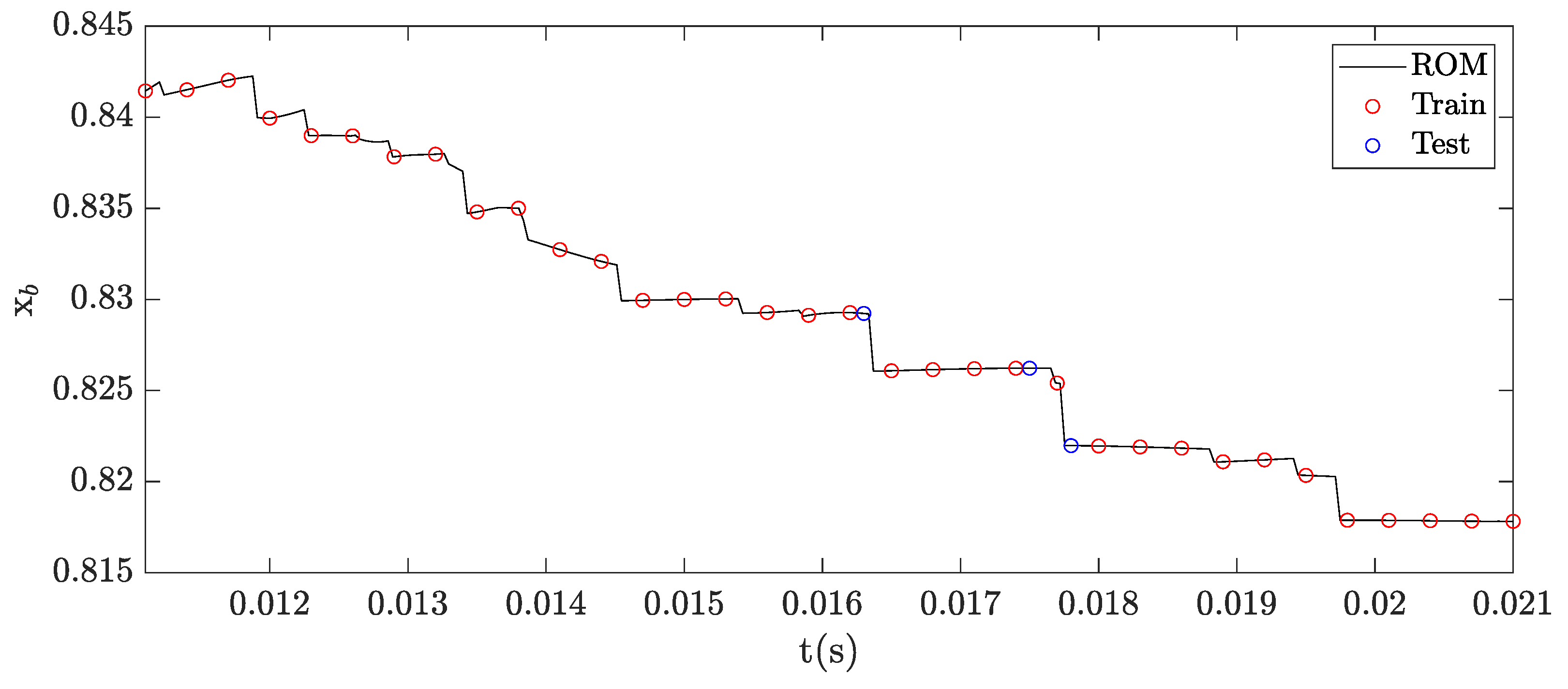
It is also worth noting that other vortex core lines were extracted, which are linked to the additional vortices forming near the surface of the body [47,48,49] and other spurious vortex lines. Therefore, the lines reported in Figure 16 are the ones resulting from the extraction procedure restricted only to the region of interest, i.e., a box containing the main leading edge vortices. Figure 17 reports the x coordinate (streamwise) of the vortex breakdown location in time, within the entire investigated time window. It can be noted how the adaptive ROM is able to catch with CFD-like accuracy the dynamics of the vortex breakdown position within the training points. Indeed, the three blue circles on the plot, the test points computed by means of CFD, fall almost exactly on the black line, which represents instead the ROM reconstructed solution. The training points are also reported on the plot, and they are highlighted with red circles. Since the adaptive ROM retains all the snapshots’ information (all modes are retained), the black line passes exactly through the training points. This would not be the case when a further reduction is forced and a subset of modes is used instead of all the ones available.
The jumps on the vortex breakdown station are not linked to the specific adaptive ROM implemented. This is supported by the additional CFD test points placed on the ROM curve in Figure 17 and also from the time evolution of conservative variables reported in Figure 18, which are the quantities directly reconstructed by the adaptive ROM. The first column in Figure 18 reports the ROM reconstructed solution for all the conservative variables (continuous blue line), together with training points (points in red) and a set of test points (points in black); the second column reports the specific method selected by the adaptive framework. It can be noted how the adaptive ROM is able to reconstruct the different variables continuously in time, also within time sub-intervals where there is a switching of methods. The jumps are therefore mainly related to the extraction technique used and the mesh resolution achievable with the computational resources available for the present work. Nevertheless, the results reported support an important capability of the adaptive ROM, which is reconstructing with CFD-like accuracy the dynamics of complex flow fields, such as the one associated with the vortex breakdown over a delta wing, with a finer resolution in time with respect to the one provided by the original set of available snapshots.
7. Vortex Dynamics for Delta Wings in a Formation Flight
A configuration of three delta wings in a formation flight was considered as the last application of the adaptive ROM. Each delta wing had the same geometry as the one used for the delta wing test case presented in Section 6. The configuration was symmetric, with one leader and two followers symmetrically positioned with respect to the leader longitudinal axis, next to the leader’s wake. There was no relative rotation among the different bodies, which therefore exhibited the same angle of attack with respect to the free stream direction. The parameters used for the unsteady simulation are summarised in Table 4.
A hybrid mesh with 15,911,216 elements and 3,824,705 grid points was used with a refinement in the region of the leader’s wake and near the interaction with the follower delta wing. A constant time step, s was used. The Reynolds-averaged Navier–Stokes equations were solved with a SST turbulence model, using a second-order finite volume discretisation for the fluxes (MUSCL approach) and a second-order dual-time stepping scheme to deal with the unsteady part. A few snapshots are reported in Figure 19 that describe the time evolution of the flow field in terms of Q-criterion isosurfaces.
The sampling to build the reduced model was performed on the time window s, which contains both the strong initial transient and the dynamics linked to the interaction of the leading edge vortex detaching from the leader with the leading edge vortex forming on the followers’ geometries. Within this time frame, a sampling of s was used, which resulted in a number of snapshots equally spaced in time. The time required for the database generation was approximately 18,000 core hours.
Figure 20 reports the quantity for the adaptive ROM in red and POD in black. For this last test case also, it can be observed how the adaptive framework performed better overall than a single POD in terms of , especially when using very few modes. Figure 21 reports the contours of , and conclusions similar to the ones reported for the previous test cases can be drawn. In particular, it can be noticed from these contours how the adaptive framework introduced major improvements in terms of residual error, when a small subset of modes is used, in the region where the interaction of trailing vortices is happening, namely the yellow-coloured regions in Figure 21.
In order to assess the actual improvement of the adaptive framework with respect to a single ROM, 15 modes out of 100 were retained to build the adaptive ROM. With this number of modes, the time required for the extraction of the set of features for the adaptive framework and the computation of the residual database was approximately 20 h (most of the time was required to extract the RDMD basis), while the extraction of the POD basis required less than one minute (no residual database required), both on a single core. The time required for one residual evaluation to generate the residual database was s on a single core, as opposed to the 60 core hours required to compute one additional CFD solution. Finally, the online phase required for both the adaptive framework and the single POD a few seconds to reconstruct the ROM solution at each desired time.
Figure 22 reports the residual evaluation in time for the entire set of conservative variables (excluding turbulence), for the three methods in the adaptive framework (left column) and the choice of these methods over the investigated time window (bar plot in the right column). It is observed how RDMD performs better for almost the entire set of conservative variables in the second half of the investigated time window, where the interaction of vortices is happening. Only for the specific case of the Z component of momentum , the different methods within the adaptive framework are almost equally chosen across the entire time interval shown. The steep increase in the RDMD residual at the end of the time window can still be linked to the interpolation issues of the RBF at the border, due to the slowly varying dynamics of the RDMD modes. The slightly increasing trend of the POD and DMD residual towards the end of the time window can be instead linked to the specific dynamics considered. The first half of the time window ( s) contains the dynamics associated with the propagation of the trailing edge vortices and the main interaction of the trailing edge vortex of the leader with the two trailing edge vortices of the follower. The few POD and DMD modes retained mainly describe such dynamics, whereas they resolve with less accuracy the dynamics happening after the main interaction, which represents a less energetic dynamics for POD, which is also dumped by the DMD eigenvalues as time increases.
The major improvements of the RDMD, and therefore of the adaptive framework, in describing the dynamics of interacting vortices can be observed in Figure 23, where the contours of the CFD reference solutions are compared with the contours of the adaptive and pure POD reconstruction on a specific slice, taken at 0.45 m from the symmetry plane. A few instants of time are shown where the interaction of vortices is happening. Superior accuracy is observed almost everywhere over the shown slice and for the various time instants. In particular, the details of the interaction region are reported in Figure 24, where it is still clearly visible how the adaptive ROM is able to resolve better the dynamics of the interaction. The improvements are measured locally in terms of how close the contours of the ROM solution are to the reference CFD solution and in integral terms using the residuals reported in Figure 22. Even if single POD appears to be good enough for some time instants, the adaptive framework is still able to introduce more details in the description of the dynamics, which is believed to be important when problems related to flow control or the design of aerodynamic surfaces is addressed.
8. Conclusions
The present work introduced both a mathematical and numerical formulation of a data-driven adaptive ROM approach employing a residual error metric to drive the selection of the set of basis functions when the solution at untried instants of time is needed. Additional residual metrics were also introduced to investigate the performance of the adaptive framework with respect to a single ROM as the number of modes is varied. Two two-dimensional unsteady test cases, namely NACA0009 and 30P30N, were used to demonstrate key elements of the adaptive framework, and two three-dimensional cases were introduced to illustrate the performance of the adaptive approach in resolving the dynamics of three-dimensional vortices generated by delta wing configurations. We discussed how the adaptive framework overall outperforms a single ROM (specifically POD) and that substantial improvements can be achieved with respect to the single ROM when using very few modes among the ones available. An explanation of the nonmonotonic behaviour with the number of modes appearing in the plots of was also provided looking at some flow field reconstructions (see Figure 3 and Figure 8). From these reconstructions, it emerged that resolving only for very large spatial structures, i.e., when using very few modes, produces a residual error from Equation (12) that is comparable with a case where other modes are added. Indeed, in the former case, a solution was obtained that solves only for large spatial features, while in the former case, the reconstructed solution solves for more spatial structures, namely the smaller ones, but also introduces spurious oscillation in the flow field. These spurious oscillations are not only due to the low resolution of existing spatial structures, but they are also linked to the advective nature of the problems, as is clearly visible from Figure 8, left, where spurious spatial oscillations appear in regions where physical quantities are transported. In addition to the above remarks, there is also a common behaviour observed in Figure 9, Figure 13, and Figure 21, while in Figure 4, the trend is different. This is worthwhile to discuss as a relation can be uncovered between the performance of the framework and the type of flow considered, due to the properties of ROMs in this work. Most apparent in the 30P30N test case, it can be observed in Figure 9 that for the initial time steps, POD performs best, especially as the number of modes is increased, but at later time instants, DMD and RDMD start performing better even when all modes are used. From Figure 6, it follows that the initial phase is highly nonlinear; however, as time progresses, the flow becomes almost steady near the airfoil, and the vortex is propagated downstream. As such, DMD and RDMD perform better where the time evolution is more linear since they are able to leverage the temporal correlation hidden in the snapshots, whereas POD is better able to approximate the highly nonlinear phase. In contrast to this, for the NACA0009 case, this state is never reached, since vortices are generated and shed continuously, as seen in Figure 1. At some time instants, the flow presents more nonlinearities, whereas at some other time instants, it is more linear. A similar behaviour is observed in Figure 4, i.e., at some time instants, POD is best, whereas at others, DMD and RDMD perform better. The above remarks indicate a potential avenue of future development, specifically the assessment of the behaviour of different ROM methods for certain types of flows.
Considering the whole analysis reported, the following conclusions can be drawn:
- -
- The residual error metric represents a relevant measure to use in order to build the adaptive ROM, since it has shown enough consistency in terms of providing the best accuracy of the final flow field reconstructions among the methods available in the framework;
- -
- A significant reduction of the problem () can be achieved through the adaptive framework, while retaining good consistency and accuracy with the physics of unsteady vortex-dominated flows. In particular, it was shown that, using a small subset of the entire set of modes that can in principle be extracted from the original snapshots, the adaptive ROM is capable of providing major improvements with respect to a single ROM based on the classical POD method. Indeed, the truncation procedure, i.e., the number of modes finally retained, which is the fundamental step to promote dimensionality reduction, is the main aspect responsible in POD for the lack of dynamic information, as the energy ranking might hide the dynamics of some low-energy spatial structures. The more detailed description of the flow field provided by the adaptive ROM is believed to be an advantage for problems that require more refined solutions, e.g., flow control and design problems;
- -
- The adaptive ROM is able to enrich the time dynamics. It was shown, indeed, how the model is able to provide a CFD-like description of the vortex breakdown displacement for the delta wing test case also outside of the training points.
Author Contributions
Conceptualization, methodology, software, validation, formal analysis, investigation, resources, data curation, writing original draft preparation, P.N.; review and editing, visualization, supervision, project administration, funding acquisition, M.F. All authors have read and agreed to the published version of the manuscript.
Funding
This research was part of the RHEA project that has received funding from the Clean Sky 2 Joint Undertaking (JU) under grant agreement No 883670. The JU receives support from the European Unions Horizon 2020 research and innovation programme and the Clean Sky 2 JU members other than the Union.
Institutional Review Board Statement
Not applicable.
Informed Consent Statement
Not applicable.
Data Availability Statement
Not applicable.
Conflicts of Interest
The authors declare no conflict of interest.
References
- Bui-Thanh, T.; Damodaran, M.; Willcox, K. Proper Orthogonal Decomposition extensions for parametric applications in compressible aerodynamics. In Proceedings of the 21st AIAA Applied Aerodynamics Conference, Orlando, FL, USA, 23–26 June 2003; p. 4213. [Google Scholar]
- Iuliano, E.; Quagliarella, D. Proper orthogonal decomposition, surrogate modelling and evolutionary optimization in aerodynamic design. Comput. Fluids 2013, 84, 327–350. [Google Scholar] [CrossRef]
- Lucia, D.J.; Beran, P.S.; Silva, W.A. Reduced-order modelling: New approaches for computational physics. Prog. Aerosp. Sci. 2004, 40, 51–117. [Google Scholar] [CrossRef] [Green Version]
- Lieu, T.; Farhat, C.; Lesoinne, M. POD-based aeroelastic analysis of a complete F-16 configuration: ROM adaptation and demonstration. In Proceedings of the 46th AIAA/ASME/ASCE/AHS/ASC Structures, Structural Dynamics and Materials Conference, Austin, TX, USA, 18–21 April 2005; p. 2295. [Google Scholar]
- Quarteroni, A.; Rozza, G. Reduced Order Methods for Modelling and Computational Reduction; Springer: Berlin/Heidelberg, Germany, 2014; Volume 9. [Google Scholar]
- Holmes, P.; Lumley, J.L.; Berkooz, G.; Rowley, C.W. Turbulence, Coherent Structures, Dynamical Systems and Symmetry; Cambridge University Press: Cambridge, UK, 2012. [Google Scholar]
- Noack, B.R. From snapshots to modal expansions–bridging low residuals and pure frequencies. J. Fluid Mech. 2016, 802, 1–4. [Google Scholar] [CrossRef] [Green Version]
- Schmid, P.J. Dynamic Mode Decomposition of numerical and experimental data. J. Fluid Mech. 2010, 656, 5–28. [Google Scholar] [CrossRef] [Green Version]
- Sieber, M.; Paschereit, C.O.; Oberleithner, K. Spectral Proper Orthogonal Decomposition. J. Fluid Mech. 2016, 792, 798–828. [Google Scholar] [CrossRef] [Green Version]
- Lumley, J.L. The structure of inhomogeneous turbulence. Atmospheric Turbulence and Radio Wave Propagation; Publishing House Nauka: Moscow, Russia, 1967; pp. 66–178. [Google Scholar]
- Berkooz, G.; Holmes, P.; Lumley, J.L. The proper orthogonal decomposition in the analysis of turbulent flows. Annu. Rev. Fluid Mech. 1993, 25, 539–575. [Google Scholar] [CrossRef]
- Luchtenburg, D.; Noack, B.; Schlegel, M. An Introduction to the POD Galerkin Method for Fluid Flows with Analytical Examples and MATLAB Source Codes; Berlin Institute of Technology: Berlin, Germany, 2009. [Google Scholar]
- Stabile, G.; Hijazi, S.; Mola, A.; Lorenzi, S.; Rozza, G. POD-Galerkin reduced order methods for CFD using Finite Volume Discretisation: Vortex shedding around a circular cylinder. Commun. Appl. Ind. Math. 2017, 8, 210–236. [Google Scholar] [CrossRef] [Green Version]
- Lorenzi, S.; Cammi, A.; Luzzi, L.; Rozza, G. POD-Galerkin method for finite volume approximation of Navier–Stokes and RANS equations. Comput. Methods Appl. Mech. Eng. 2016, 311, 151–179. [Google Scholar] [CrossRef]
- Fossati, M.; Habashi, W.G. Multiparameter analysis of aero-icing problems using proper orthogonal decomposition and multidimensional interpolation. AIAA J. 2013, 51, 946–960. [Google Scholar] [CrossRef]
- Buljak, V. Proper orthogonal decomposition and radial basis functions for fast simulations. In Inverse Analyses with Model Reduction; Springer: Berlin/Heidelberg, Germany, 2012; pp. 85–139. [Google Scholar]
- Walton, S.; Hassan, O.; Morgan, K. Reduced order modelling for unsteady fluid flow using proper orthogonal decomposition and radial basis functions. Appl. Math. Model. 2013, 37, 8930–8945. [Google Scholar] [CrossRef]
- Mohan, A.T.; Gaitonde, D.V. A deep learning based approach to reduced order modelling for turbulent flow control using LSTM neural networks. arXiv 2018, arXiv:1804.09269. [Google Scholar]
- Gao, Z.; Liu, Q.; Hesthaven, J.; Wang, B.; Don, W.; Wen, X. Non-intrusive reduced order modelling of convection dominated flows using artificial neural networks with application to Rayleigh-Taylor instability. Commun. Comput. Phys. 2022, 30, 97–123. [Google Scholar] [CrossRef]
- Wang, Z.; Xiao, D.; Fang, F.; Govindan, R.; Pain, C.C.; Guo, Y. Model identification of reduced order fluid dynamics systems using deep learning. Int. J. Numer. Methods Fluids 2018, 86, 255–268. [Google Scholar] [CrossRef] [Green Version]
- Hesthaven, J.S.; Ubbiali, S. Non-intrusive reduced order modelling of nonlinear problems using neural networks. J. Comput. Phys. 2018, 363, 55–78. [Google Scholar] [CrossRef] [Green Version]
- Liang, Y.; Lee, H.; Lim, S.; Lin, W.; Lee, K.; Wu, C. Proper Orthogonal Decomposition and its applications—Part I: Theory. J. Sound Vib. 2002, 252, 527–544. [Google Scholar] [CrossRef]
- Rowley, C.W. Model reduction for fluids, using balanced Proper Orthogonal Decomposition. Int. J. Bifurc. Chaos 2005, 15, 997–1013. [Google Scholar] [CrossRef] [Green Version]
- Noack, B.R.; Stankiewicz, W.; Morzyński, M.; Schmid, P.J. Recursive Dynamic Mode Decomposition of transient and post-transient wake flows. J. Fluid Mech. 2016, 809, 843–872. [Google Scholar] [CrossRef] [Green Version]
- Cazemier, W.; Verstappen, R.; Veldman, A. Proper Orthogonal Decomposition and low-dimensional models for driven cavity flows. Phys. Fluids 1998, 10, 1685–1699. [Google Scholar] [CrossRef] [Green Version]
- Kutz, J.N.; Fu, X.; Brunton, S.L. Multi-Resolution Dynamic Mode Decomposition. arXiv 2015, arXiv:math.DS/1506.00564. [Google Scholar]
- Le Clainche, S.; Vega, J. Higher Order Dynamic Mode Decomposition. SIAM J. Appl. Dyn. Syst. 2017, 16, 882–925. [Google Scholar] [CrossRef] [Green Version]
- Pascarella, G.; Kokkinakis, I.; Fossati, M. Analysis of Transition for a Flow in a Channel via Reduced Basis Methods. Fluids 2019, 4, 202. [Google Scholar] [CrossRef] [Green Version]
- Pascarella, G.; Fossati, M.; Barrenechea, G. Adaptive reduced basis method for the reconstruction of unsteady vortex-dominated flows. Comput. Fluids 2019, 190, 382–397. [Google Scholar] [CrossRef]
- Amsallem, D.; Zahr, M.J.; Farhat, C. Nonlinear model order reduction based on local reduced-order bases. Int. J. Numer. Methods Eng. 2012, 92, 891–916. [Google Scholar] [CrossRef]
- Carlberg, K. Adaptive h-refinement for reduced-order models. Int. J. Numer. Methods Eng. 2015, 102, 1192–1210. [Google Scholar] [CrossRef] [Green Version]
- Washabaugh, K.; Amsallem, D.; Zahr, M.; Farhat, C. Nonlinear model reduction for CFD problems using local reduced-order bases. In Proceedings of the 42nd AIAA Fluid Dynamics Conference and Exhibit, New Orleans, LA, USA, 25–28 June 2012; p. 2686. [Google Scholar]
- Viana, F.; Haftka, R.; Steffen, V., Jr. Multiple surrogates: How cross-validation errors can help us to obtain the best predictor. Struct. Multidiscip. Optim. 2009, 39, 439–457. [Google Scholar] [CrossRef]
- Pascarella, G.; Fossati, M. Model-Based Adaptive MOR Framework for Unsteady Flows Around Lifting Bodies. In Model Reduction of Complex Dynamical Systems; Benner, P., Breiten, T., Faßbender, H., Hinze, M., Stykel, T., Zimmermann, R., Eds.; Springer International Publishing: Berlin/Heidelberg, Germany, 2021; pp. 283–305. [Google Scholar] [CrossRef]
- Economon, T.D.; Palacios, F.; Copeland, S.R.; Lukaczyk, T.W.; Alonso, J.J. SU2: An open-source suite for multiphysics simulation and design. AIAA J. 2015, 54, 828–846. [Google Scholar] [CrossRef]
- Sirovich, L. Method of snapshots. Q. Appl. Math. 1987, 45, 561–571. [Google Scholar] [CrossRef] [Green Version]
- Tu, J.H.; Rowley, C.W.; Luchtenburg, D.M.; Brunton, S.L.; Kutz, J.N. On Dynamic Mode Decomposition: Theory and applications. arXiv 2013, arXiv:1312.0041. [Google Scholar]
- Jovanović, M.R.; Schmid, P.J.; Nichols, J.W. Sparsity-promoting Dynamic Mode Decomposition. Phys. Fluids 2014, 26, 24103. [Google Scholar] [CrossRef]
- Carr, J.C.; Beatson, R.K.; Cherrie, J.B.; Mitchell, T.J.; Fright, W.R.; McCallum, B.C.; Evans, T.R. Reconstruction and representation of 3D objects with radial basis functions. In Proceedings of the 28th Annual Conference on Computer Graphics and Interactive Techniques, San Antonio, TX, USA, 23–26 July 2001; pp. 67–76. [Google Scholar]
- Allendes, A.; Barrenechea, G.R.; Rankin, R. Fully computable error estimation of a nonlinear, positivity-preserving discretization of the convection-diffusion-reaction equation. SIAM J. Sci. Comput. 2017, 39, A1903–A1927. [Google Scholar] [CrossRef] [Green Version]
- Chu, J.; Luckring, J.M. Experimental Surface Pressure Data Obtained on 65 Delta Wing across Reynolds Number and Mach Number Ranges; National Aeronautics and Space Administration, Langley Research Center: Hampton, VA, USA, 1996.
- Lin, J.C.; Rockwell, D. Transient structure of vortex breakdown on a delta wing. AIAA J. 1995, 33, 6–12. [Google Scholar] [CrossRef]
- Kumar, A. On the structure of vortex breakdown on a delta wing. Proc. R. Soc. Lond. Ser. A Math. Phys. Eng. Sci. 1998, 454, 89–110. [Google Scholar] [CrossRef]
- Roth, M.; Peikert, R. A higher-order method for finding vortex core lines. In Proceedings of the Visualization’98 (Cat. No. 98CB36276), Research Triangle Park, NC, USA, 18–23 October 1998; pp. 143–150. [Google Scholar]
- Peikert, R.; Roth, M. The parallel vectors operator-a vector field visualization primitive. In Proceedings of the Visualization’99 (Cat. No. 99CB37067), San Francisco, CA, USA, 24–29 October 1999; pp. 263–532. [Google Scholar]
- Sujudi, D.; Haimes, R. Identification of swirling flow in 3-D vector fields. In Proceedings of the 12th Computational Fluid Dynamics Conference, San Diego, CA, USA, 19–22 June 1995; p. 1715. [Google Scholar]
- Lee, M.; Ho, C.M. Vortex dynamics of delta wings. In Frontiers in Experimental Fluid Mechanics; Springer: Berlin/Heidelberg, Germany, 1989; pp. 365–427. [Google Scholar]
- Agrawal, S.; Barnett, R.M.; Robinson, B.A. Numerical investigation of vortex breakdown on a delta wing. AIAA J. 1992, 30, 584–591. [Google Scholar] [CrossRef]
- Visbal, M. Computational and physical aspects of vortex breakdown on delta wings. In Proceedings of the 33rd Aerospace Sciences Meeting and Exhibit, Reno, NV, USA, 9–12 January 1995; p. 585. [Google Scholar]
Figure 1.
Contours of the Mach number for the impulsive start over the NACA0009 airfoil at different instants of time. Left to right, top to bottom: , , , , , s.
Figure 1.
Contours of the Mach number for the impulsive start over the NACA0009 airfoil at different instants of time. Left to right, top to bottom: , , , , , s.

Figure 2.
The varying the number of modes, for adaptive ROM and POD, NACA0009 test case.

Figure 3.
Volume reconstruction of density at time s for 2 modes (left) and 28 modes (right), NACA0009 test case. Black contours represent the CFD reference solution; red contours represent the ROM reconstructed solution.
Figure 3.
Volume reconstruction of density at time s for 2 modes (left) and 28 modes (right), NACA0009 test case. Black contours represent the CFD reference solution; red contours represent the ROM reconstructed solution.

Figure 4.
The considering POD as the reference single ROM, versus the time and number of modes, NACA0009 test case. White regions correspond to , i.e., the residual based adaptive ROM selects POD.
Figure 4.
The considering POD as the reference single ROM, versus the time and number of modes, NACA0009 test case. White regions correspond to , i.e., the residual based adaptive ROM selects POD.

Figure 5.
Comparison of the volume solution in terms of . Coloured lines show the ROM reconstruction, while the black lines show the reference CFD solution. The left column shows the adaptive reconstruction, and the right column shows the pure POD reconstruction, both computed retaining 10 modes.
Figure 5.
Comparison of the volume solution in terms of . Coloured lines show the ROM reconstruction, while the black lines show the reference CFD solution. The left column shows the adaptive reconstruction, and the right column shows the pure POD reconstruction, both computed retaining 10 modes.

Figure 6.
Contours of pressure for the impulsive start over the 30P30N airfoil at different instants of time.
Figure 6.
Contours of pressure for the impulsive start over the 30P30N airfoil at different instants of time.

Figure 7.
The varying the number of modes, for adaptive ROM and POD, 30P30N test case.

Figure 8.
Volume reconstruction of density at time s for 6 modes (left) and 17 modes (right), 30P30N test case. Black contours represent the CFD reference solution; red contours represent the ROM reconstructed solution.
Figure 8.
Volume reconstruction of density at time s for 6 modes (left) and 17 modes (right), 30P30N test case. Black contours represent the CFD reference solution; red contours represent the ROM reconstructed solution.

Figure 9.
The considering POD as the reference single ROM, versus the time and number of modes, 30P30N test case. White regions correspond to , i.e., the residual based adaptive ROM selects POD.
Figure 9.
The considering POD as the reference single ROM, versus the time and number of modes, 30P30N test case. White regions correspond to , i.e., the residual based adaptive ROM selects POD.

Figure 10.
Comparison of the volume solution in terms of . Coloured lines show the ROM reconstruction, while the black lines show the reference CFD solution. The left column shows the adaptive reconstruction; the right columns shows the pure POD reconstruction.
Figure 10.
Comparison of the volume solution in terms of . Coloured lines show the ROM reconstruction, while the black lines show the reference CFD solution. The left column shows the adaptive reconstruction; the right columns shows the pure POD reconstruction.

Figure 11.
Contours of the Q-criterion s−2 coloured with the velocity magnitude for different time instants, delta wing test case.
Figure 11.
Contours of the Q-criterion s−2 coloured with the velocity magnitude for different time instants, delta wing test case.

Figure 12.
The varying the number of modes, for adaptive ROM and POD, delta wing test case.

Figure 13.
The considering POD only single ROM, versus the time and number of modes, delta wing test case. White regions correspond to , i.e., the adaptive ROM selects POD.
Figure 13.
The considering POD only single ROM, versus the time and number of modes, delta wing test case. White regions correspond to , i.e., the adaptive ROM selects POD.

Figure 14.
Volume residual evaluation (left column) and choice of methods (right columns) for all the conservative variables (excluding turbulence), fixed number of modes , delta wing test case.
Figure 14.
Volume residual evaluation (left column) and choice of methods (right columns) for all the conservative variables (excluding turbulence), fixed number of modes , delta wing test case.

Figure 15.
Comparison of volume solution in terms of for the delta wing test case. The black contours report the CFD reference solution; the coloured contour lines show the ROM reconstruction. The left column shows the adaptive reconstruction; the right column shows the pure POD reconstruction. Number of modes fixed, .

Figure 16.
Vortex core lines associated with the main leading edge vortices, extracted through the vortex core tool of Paraview 5.9.0. Surface contours represent surface pressure.
Figure 16.
Vortex core lines associated with the main leading edge vortices, extracted through the vortex core tool of Paraview 5.9.0. Surface contours represent surface pressure.

Figure 17.
Displacement of vortex breakdown station within the investigated time window. The continuous line represents the ROM; the red circles are the training snapshots; the blue circles represent the test points.
Figure 17.
Displacement of vortex breakdown station within the investigated time window. The continuous line represents the ROM; the red circles are the training snapshots; the blue circles represent the test points.

Figure 18.
Evolution of the conserved quantities (left column) and methods selected by the adaptive framework (right column), within the time window investigated for the vortex breakdown in the delta wing test case. The continuous line represents the ROM; the red points are the training snapshots; the black points are the test points.

Figure 19.
Contours of the Q-criterion s−2 coloured with the velocity magnitude () for different time instants, formation flight test case.
Figure 19.
Contours of the Q-criterion s−2 coloured with the velocity magnitude () for different time instants, formation flight test case.

Figure 20.
The varying the number of modes, for adaptive ROM and POD, formation flight test case.

Figure 21.
The considering POD as the reference single ROM, versus time and number of modes, formation flight test case. White regions correspond to , i.e., the model based adaptive ROM selects POD.
Figure 21.
The considering POD as the reference single ROM, versus time and number of modes, formation flight test case. White regions correspond to , i.e., the model based adaptive ROM selects POD.

Figure 22.
Volume residual evaluation (left column) and choice of methods (right columns) for all the conservative variables (excluding turbulence), fixed number of modes , formation flight test case.
Figure 22.
Volume residual evaluation (left column) and choice of methods (right columns) for all the conservative variables (excluding turbulence), fixed number of modes , formation flight test case.

Figure 23.
Comparison of the volume solution in terms of for the formation flight test case. The black contours report the CFD reference solution; the coloured contour lines show the ROM reconstruction. The left column shows the adaptive reconstruction; the right column shows the pure POD reconstruction. Slice taken at 0.45 m from the plane of symmetry. Number of modes fixed, .

Figure 24.
Detail of the volume solution in the region of vortices’ interaction, in terms of for the formation flight test case. The black contours report the CFD reference solution; the coloured contour lines show the ROM reconstruction. The left column shows the adaptive reconstruction; the right column shows the pure POD reconstruction. Slice taken at m from the plane of symmetry. Number of modes fixed, .


Table 1.
NACA0009 simulation parameters.
| Mach | (deg) | Reynolds | (K) | Time (s) | (s) | CFL |
|---|---|---|---|---|---|---|
| 0.1 | 15 | 10,000 | 288.15 | 0.3 | 10−3 | 5 |
Table 2.
The 30P30N simulation parameters.
| Mach | (deg) | Reynolds | (K) | Time (s) | (s) | CFL |
|---|---|---|---|---|---|---|
| 0.2 | 19 | 300 | 0.03 | 10−4 | 0.4 |
Table 3.
Delta wing simulation parameters.
| Mach | (deg) | Reynolds | (K) | Time (s) | (s) | CFL |
|---|---|---|---|---|---|---|
| 0.4 | 23 | 288.0 | 0.021 | 10−4 | 0.5 |
Table 4.
Formation flight simulation parameters.
| Mach | (deg) | Reynolds | (K) | Time (s) | (s) | CFL |
|---|---|---|---|---|---|---|
| 0.4 | 15 | 288.0 | 0.021 | 10−4 | 1 |
Publisher’s Note: MDPI stays neutral with regard to jurisdictional claims in published maps and institutional affiliations. |
© 2022 by the authors. Licensee MDPI, Basel, Switzerland. This article is an open access article distributed under the terms and conditions of the Creative Commons Attribution (CC BY) license (https://creativecommons.org/licenses/by/4.0/).
Share and Cite
MDPI and ACS Style
Nagy, P.; Fossati, M. Adaptive Data-Driven Model Order Reduction for Unsteady Aerodynamics. Fluids 2022, 7, 130. https://0-doi-org.brum.beds.ac.uk/10.3390/fluids7040130
AMA Style
Nagy P, Fossati M. Adaptive Data-Driven Model Order Reduction for Unsteady Aerodynamics. Fluids. 2022; 7(4):130. https://0-doi-org.brum.beds.ac.uk/10.3390/fluids7040130
Chicago/Turabian StyleNagy, Peter, and Marco Fossati. 2022. "Adaptive Data-Driven Model Order Reduction for Unsteady Aerodynamics" Fluids 7, no. 4: 130. https://0-doi-org.brum.beds.ac.uk/10.3390/fluids7040130