
Hydrodynamic Characteristics of Two Side-by-Side Cylinders at a Pitch Ratio of 2 at Low Subcritical Reynolds Numbers
Group of Experimental and Computational Mechanics, University of Brasília, Gama 72.405-610, Brazil
*
Author to whom correspondence should be addressed.
Fluids 2022, 7(9), 287; https://0-doi-org.brum.beds.ac.uk/10.3390/fluids7090287
Submission received: 17 May 2022
/
Revised: 2 August 2022
/
Accepted: 3 August 2022
/
Published: 30 August 2022
(This article belongs to the Topic Fluid Mechanics)
Abstract
:Isothermal turbulent flow around circular cylinders arranged side-by-side was numerically simulated on a commercial finite-volumes platform, ANSYS® CFX, version 2020 R2. The turbulence was modeled by using k-ω shear stress transport (k-ω SST). Three different Reynolds numbers were computed, Red = 200, 1000, and 3000, which were based on the cylinder diameter, d, the free stream velocity, U∞, and the kinematic viscosity of the fluid, ν. Sided cylinders were spaced apart from each other, forming a p/d ratio equal to 2, which was kept constant throughout the computations regardless of changes in the Reynolds number. The drag coefficient, Cd, as well as its time traces, was evaluated along with the different wake topologies experienced by the cylinders (wide wake WW and narrow wake NW). The simulations were able to predict the bistable flow over the cylinders and the Cd changes associated with the wakes. Whenever a new wake topology was identified, the shape drag changed in accordance with the instantaneous pressure distribution. A laminar simulation was carried out for the lowest Reynolds number case, showing that the adopted turbulence model did not affect the dynamic response of the flow. The Red = 3000 case was compared to Afgan’s outcomes, whose simulations were carried out in a 3-D mesh using LES (Large Eddy Simulation), showing great agreement with their results.
1. Introduction
Due to vast applications in real life, the study of turbulent flow characteristics around cylinders has been the focus of attention for a long time. Knowledge of the flow field and its dynamics characteristics over such bodies is applied on a vast scale. Circular cylinders in pairs (side-by-side or in tandem) or even arranged in banks have been the subject of research since the very early twentieth century with the outcomes released by Grimison [1] and Wiemer [2]. A very thorough experimental campaign was carried out by Žukauskas [3], followed by Žukauskas et al. [4] and Žukauskas and Katinas [5]. In these works, the authors were very concerned with outlining the basis for heat transfer prediction in bank tubes, for instance in Žukauskas’s work [3]. It is important to remind the reader that bank tubes or closed packet rods are the simplest geometries used for research to study the flow field and the features of its fluctuation over structures arranged in groups. We can easily cite the case of struts of a biplane wing or the flow past columns of a marine structure in offshore engineering, transmission lines, and heat exchanger tubes or bundles of risers [6,7]. In contrast to the high Reynolds numbers produced in such applications, low Reynolds numbers can be seen in the papermaking process [8]. According to the authors, the wood fibers can be modelled as sided cylindrical structures with dimensions of about 1 mm in length and 40 μm in diameter.
In recent times, the works [9,10,11,12,13,14], among others, were concerned with the wake interactions behind the cylinders when the gap between them changes. Furthermore, they also try to understand the flow changes in association with the Reynolds numbers, as was shown very well by Sumner [14].
Bearman and Wadcok [15] investigated experimentally the flow interaction in a pair of circular cylinders for a Reynolds number of 2.5 × 10⁴. The work aimed to study the flow behavior as the p/d ratio changed. The authors observed that for sided circular cylinders separated from each other by a p/d ratio greater than 2, the wake formed downstream was similar to the one that takes place in a single cylinder. However, as the p/d ratio decreased, an asymmetric flow field appeared around the cylinder, also producing some effect on the vortex-shedding frequency. Furthermore, the authors, in 1973, also they pointed out that the shedding vortex mode could occur in phase and antiphase synchronization, but the second mode was seen more often. Years later, Meneghini and co-workers [16] also reached the same conclusion. At that time, the authors only associated this difference with the p/d ratio. Later, Zdravkovich and Pridden [7] investigated the wake formation and its relationship with the p/d ratio, reaching the same conclusions on the asymmetric flow field whenever the p/d ratio decreased below 2. Their experimental campaign conducted under subcritical Reynolds numbers (8 × 10³ to 1.6 × 10⁵) showed that different drags were assigned to the cylinders at the same time. Furthermore, the sum of the drags was less than twice the value of the drag for a single cylinder under the same Reynolds number.
Numerical and experimental works have aimed to study the bistability process in either a row of cylinders or in a pair of them [16,17,18,19]. According to Neumeister [19], bistable flow is only observed in the situation in which the wakes interact with each other, giving rise to stable wake topologies that can change randomly over time. Such a configuration leads to an asymmetric flow, forming dissimilar wakes (narrow wake NW and wide wake WW) downstream of the cylinders, whose main characteristics rule the aerodynamic forces on the cylinders’ surfaces and the dynamics of the flow as well. Asymmetric wake formation was also shown by researchers [20,21,22,23]. Vila et al. [24] carried out an experimental campaign using two hot-wire probes and a single pressure transducer in a pair of circular cylinders for three different p/d ratios. They evaluated the turbulent signals of pressure and velocity acquired at the same time. The pressure time trace was gathered on the circular cylinder’s surface, while the velocity signals were taken in the viscous wake. The authors performed this study for three different p/d ratios (1.26, 2.00, and 3.00) under a subcritical regime, Red = 1.78 × 10⁴. The authors identified that both the stagnation and boundary layer detachment points moved towards the tight gap as the p/d ratio decreased. Furthermore, with regard to the velocity and pressure time traces, the signals were seen to present long-term bistable behavior for the lowest p/d ratio. On the other hand, as the p/d ratio increased, this pattern tended to fade away. Spectral analysis using both PSD and CWT [18] tools showed energy peaks associated with the vortex shedding. The Strouhal number was seen to range from 0.22 to 0.24. These values were slightly higher than that identified in a single cylinder.
The outcomes for two-dimensional flow characteristics over circular cylinders arranged in pairs were reported by Kang [22]. In his numerical work, the author carried out simulations for various Reynolds numbers and T/D ratios, comprising 40 ≤ Re ≤ 160 and 0.2 ≤ T/D ≤ 5.0, respectively. Unlike others, the author characterized the narrow gap space between cylinders as T = p/d – 1. The numerical results of Kang [22] identified up to six different topologies for wakes, depending on the distance between the centers of the cylinders and the Reynolds number. The author also stated that, for the studied Reynolds number range, the frequency of vortex shedding was influenced mainly by the spacing between the cylinders. For 0.5 < T/D < 1.5, the vortex frequency dropped and was constantly synchronized with the movement of the wakes. On the other hand, the drag coefficients depended mainly on the spacing between the cylinders. Finally, the author concluded that as the T/D ratio increased, for values higher than 3, the flow characteristics again became significantly dependent on the Reynolds number.
In case of fluid–structure interaction (FSI), recently, Chen and co-authors [25,26] investigated the wake patterns of two-sided circular cylinders which were free to vibrate. The authors’ investigations, in both works, aimed to provide an overview of the wake patterns for different p/d ratios and Reynolds numbers, whose values ranged from 60 up to 200. In the first paper by Chen [25], the authors simulated the fluid–structure interaction by using the immersed boundary (IB) method. The gap-spacing ratio (p/d) and the reduced velocity (Ur) were changed from 2 up to 5 and 0 up to 30, respectively. The authors identified up to eight wake flow patterns, whose existence was based on the gap spacing and the reduced velocity. For instance, the biased flow, which produces narrow and wide wakes, was only observed for a 2.3 < p/d <2.5 and Ur varied between 4.0 and 4.50. Later, in 2020, Chen [26] and co-authors furthered their numerical experiments by studying the effects of the p/d ratio and the reduced velocity Ur on the flow dynamics of two-sided cylinders free to vibrate. The authors concluded that the p/d ratio plays an important role in the dynamic response of the cylinders. The authors identified St > 0.20 for low Ur and gap ratios between 2.0 and 2.5.
The present work aimed to numerically investigate the hydrodynamic characteristics over two-sided cylinders. Three Reynolds numbers were simulated, Red = 200, 1000, and 3000, keeping the p/d ratio constant, equal to 2. In order to verify the quality of the computations, mean average values such as the stagnation and separation angles, (θEst) and (δSep), and the drag forces, Cd, were compared to those reported by Afgan et al. [27] for Red = 3000 and a p/d ratio equal to 2. Finally, special attention was given to the bistability of the flow and its effect on the aerodynamic forces whenever a new topology was formed as well as the dynamic response of the flow behind the cylinders through the velocity time traces.
2. Materials and Methods
2.1. Governing Equations
For incompressible flow, the mass and the momentum conservation are ruled by:
In Equations (1) and (2), and represent the velocity vector components, is the spatial coordinates, is the thermodynamic pressure, ρ is the fluid density, and ν and νt are the molecular and turbulent kinematic viscosity, respectively. The additional momentum diffusivity caused by the closure problem of the turbulence is represented by the turbulent viscosity, νt, which is approached through Boussinesq’s idea, as follows:
is the Reynolds tensor, which comes from the decomposition of the nonlinear terms of the Navier–Stokes equation, and k represents the turbulent kinetic energy. So, additional equations are needed to model the turbulent kinematic viscosity, which is computed as a function of the turbulent kinetic energy field, k, and the specific rate of dissipation, ω.
The k-ω SST model is a two-equation turbulence model first introduced by Menter [28]. The model combines the advantages of the k-ε model and the k-ω model through a blending function that switches whenever it is possible. According to Menter [28], the two-equation model is ruled by the set of equations in Equation (4):
The bending function is F1, which computes how far from the walls the problem is:
Finally, the turbulent kinematic viscosity is calculated by
where Ω is the absolute value of the vorticity and a1 is a closure coefficient that is set to 0.30. For further information, see the complete description of the model in [28].
2.2. Computational Domain, Boundary Conditions, and Mesh Dependence
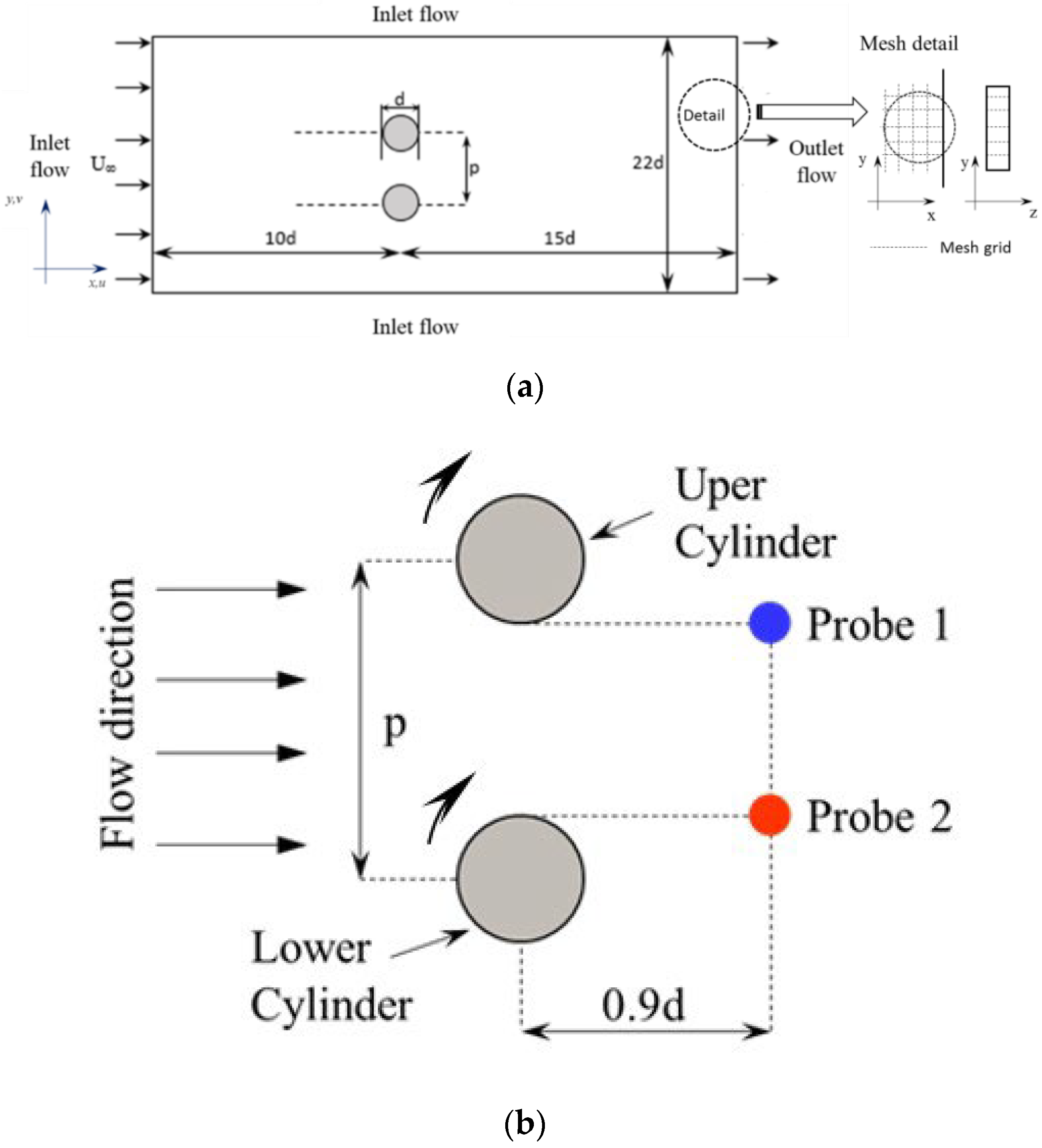
The rectangular computational domain is based on the work published by Afgan et al. [27]. Its dimensions were made dimensionless by using the diameter of the circular cylinder, d, its total length being 25d, and height 22d. From the inlet up to the cylinders’ center, the computational domain is 10d long, whereas downstream of the cylinders, the flow travels 15d to reach the domain’s outlet. Both cylinders are placed in the center of the domain. Furthermore, their centers are separated from each other by a distance, p. The dimensionless number that rules this distance is the p/d ratio, which was kept constant throughout this work, being equal to 2. The flow comes into the domain through the inlet with a free stream velocity, U∞, oriented parallel to the x-axis. A prescribed velocity, u = U∞, v = w = 0, was imposed on the upper and lower faces of the domain (Figure 1a). The free stream turbulence intensity was set to 1% (in the work by Afgan et al. [27], the authors did not provide this information). No slip condition was applied to the walls, u = v = 0, and, finally, the outlet boundary. At the outlet boundary, the pressure difference was set to zero. A schematic view of the domain, its coordinates, boundaries, and mesh detail are depicted in Figure 1a. Figure 1b shows a schematic view of the circular cylinders and how they are oriented. The arrow over the cylinders indicates how the azimuthal positions are taken into account.
Based on the entrance velocity, three Reynolds numbers were simulated, Red = 200, 1000, and 3000, keeping the domain’s dimensions, p/d ratio, and cylinder diameters unchanged. The commercial software ANSYS CFX is only able to perform analyses for 3-D domains. To ensure that the 2-D flow over the cylinders was symmetric, symmetry boundary conditions were applied to the x,y faces, which means that the spanwise derivative terms of the equations are set to zero.
Downstream of the upper and lower cylinders, two probes, i.e., points in the mesh where the temporal flow data were stored, were placed at a distance of 0.9d from the cylinder’s center (Figure 1b). The probes were placed according to the work by De Paula et al. [18]. Velocity time traces were gathered by the virtual probes.
The mesh was built by splitting the domain into smaller ones, all of which were formed of smaller hexahedral volumes. Special care was taken near the walls (on the cylinders’ surfaces), where y+ was carefully computed to ensure that the nondimensional distance from the wall would not exceed unity. The y+ was measured after each stationary run of a new mesh. Parallel to the z-axis, the mesh was built by splitting the third dimension into one volume (see the mesh detail in Figure 1a). The domain’s thickness was 10 mm. Three different meshes were built and tested for Red = 3000. Afgan et al. [27] used the same configuration and Reynolds number for predicting the turbulent flow over side-by-side circular cylinders. Their outcomes were used as a benchmark for the present simulations. In Figure 2, one can see the y+ distribution on the cylinders’ surface. It is possible to see that any generated mesh achieved the first imposition, that is y+ ≤ 1. Actually, the coarsest one showed y+ = 1 at about 45° on the lower cylinder’s surface. For the reader’s guidance, in Figure 2, the flow reached the cylinders from left to right.
As stated above, three different meshes were tested and compared with the results presented in the work by Afgan et al. [27]. The meshes were named from M3, the finest one, to M1, the coarsest. The mesh characteristics and results are summarized in Table 1, along with the stagnation (θEst) and separation angles (δSep) and the results published earlier by Afgan et al. [2]. From Table 1, it is possible to observe that the results from the meshes are quite close to those reported in Afgan’s paper. The stagnation angles (θEst) were seen to be unchanged, regardless of the mesh.
Only a very marginal difference of 0.4° is seen in comparison with Afgan’s results. The highest variations were observed for the flow separation angle, δSep. As the mesh becomes finer, the location where the flow detaches becomes closer to the value predicated by Afgan and his co-workers in their 3-D numerical simulation. The difference was found to range from 1% (M3) up to 4.70% (M1). Considering the results and the time-consuming simulation, the mesh M2 was chosen to carry out all computations. Each transient numerical simulation case took about 05 days on an i7 3.6 GHz computer with 06 cores and 32 GB of RAM.
Time-dependent computations were performed for 2900 s, which means seven flowthroughs for the highest Reynolds number. For the lowest Reynolds number, the total time was about 105 flowthroughs. The time-step for each Reynolds number was small enough to achieve a Courant number less than 1, as already carried out in the previous papers [29,30]. So, for Red = 200, 1000, and 3000, the time-step was set to 0.8, 0.14, and 0.03, respectively. During the numerical simulation, the temporal scheme was second-order backward Euler, the advective terms were discretized using an upwind second-order scheme, and the convergence criterion was set as at least 10−6 for each equation. The mean average data were averaged over the total time of the transient solution.
3. Results and Discussion
3.1. Stagnation (θEst) and Detached (δSep) Angles
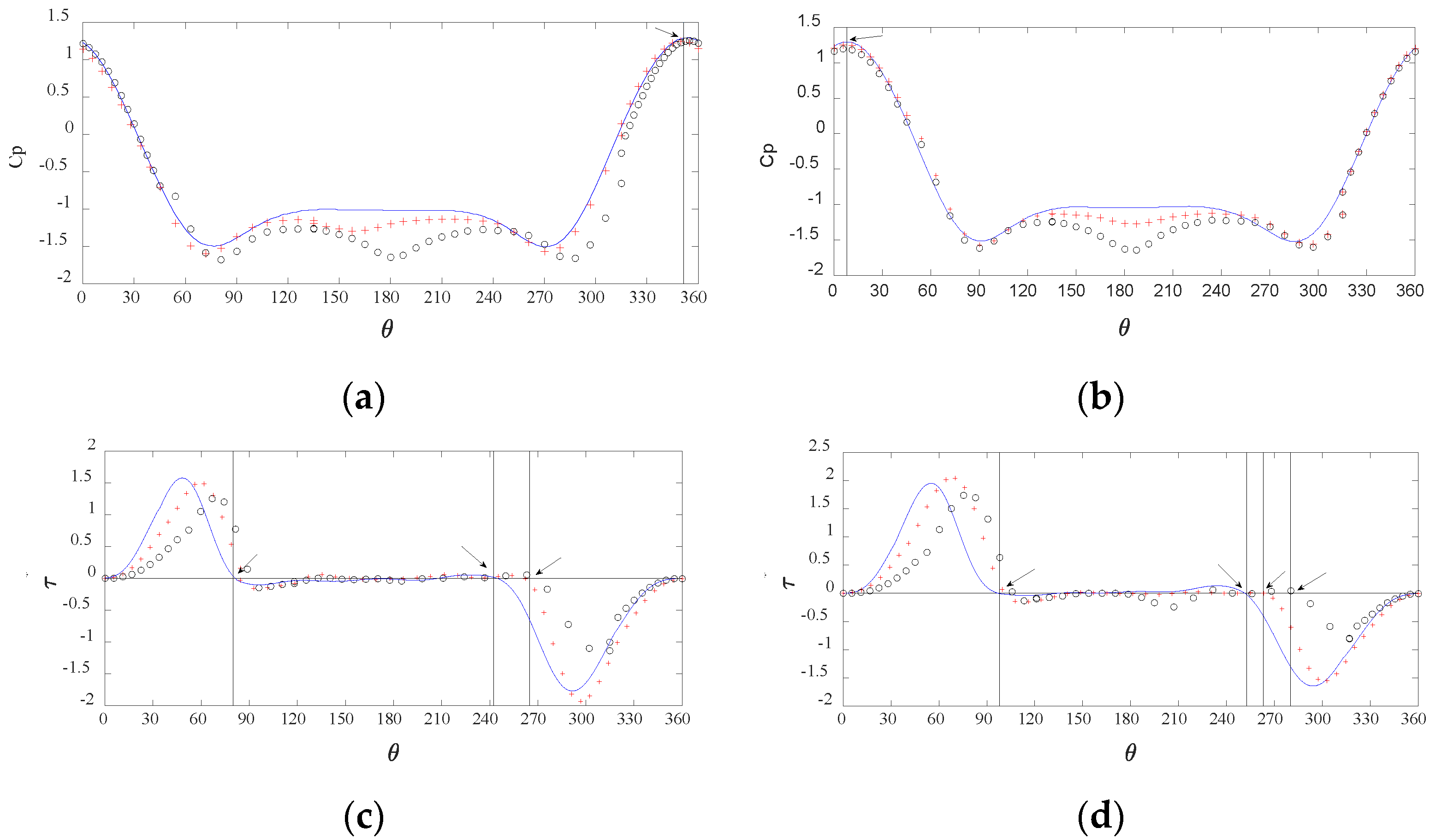
In Figure 3, mean average pressure (Figure 3a,b) and skin friction coefficients (Figure 3c,d) are shown as a function of the azimuthal position around the cylinders’ surfaces. Both the pressure coefficient, Cp, and the skin friction coefficient, τ*, were computed as shown by Achenbach [31] and Johansson [18] according to the expressions:
Focusing on the pressure distribution, one can see a similar distribution regardless of the Reynolds number. First, the stagnation point shifted towards the gap on both cylinders, taking place at about 354° and 7.70° in the upper and lower cylinders, respectively. According to the numerical work by Hensan [32], the movement of the stagnation angles is due to the repelling forces acting over the cylinders when they are close to each other. Furthermore, the repelling forces, according to the author, become stronger as the cylinders become closer. As stated before, despite the Reynolds number changing, the stagnation point location is not affected. Regarding the pressure values, the lowest coefficients occurred at different angular positions, depending on the cylinder. For the upper one (Figure 3a), the minima are placed at 75° and 285° for a Reynolds number of 3000. Moreover, regardless of the tube position, the pressure distribution fell at 180°, showing a valley for Red = 3000. In Figure 3c,d, the main purpose is to know where the boundary layer detaches. Here, the dissimilarities between the different Reynolds numbers are much more evident. In both tubes, the angle where the skin coefficient, τ*, is maximal moves downstream as the Reynolds number increases and the separation angle, δSep, identified by τ* = 0, seems to be sensitive to Reynolds number in both cylinders. According to this criterion, the boundary layers were found to detach soon after 85°, first for the lowest Reynolds number, followed by Red = 1000 and 3000, in sequence. For Reynolds numbers of 1000 and 3000, the δSep difference was found to be marginal. On the lower cylinder’s surface, the τ* distribution was found to be slightly different on the opposite side of the narrow gap. The skin friction coefficient was found to be zero at about 250° for Red = 200, followed by Red = 1000 and 3000, respectively. It is also interesting to notice that the separation angles are shifted in the narrow gap in comparison to the position where it takes place on the opposite side. The points where the boundary layer is detached are indicated by arrows in Figure 3c,d. Table 2 summarizes the stagnation and separation angles for each cylinder.
3.2. The Drag Coefficients and the Wake Interactions
The instantaneous time history of the drag coefficients in both cylinders was gathered for every Reynolds number simulated. The drag coefficient is computed based on the following expression:
where Cd is the drag coefficient and Fd is the total drag forces that are parallel to the x-axis. The circular cylinder diameter is d and is the thickness of the domain (dimension parallel to the z-axis). The time, t*, was made dimensionless by using the entrance velocity, U∞, and the cylinder’s diameter as .
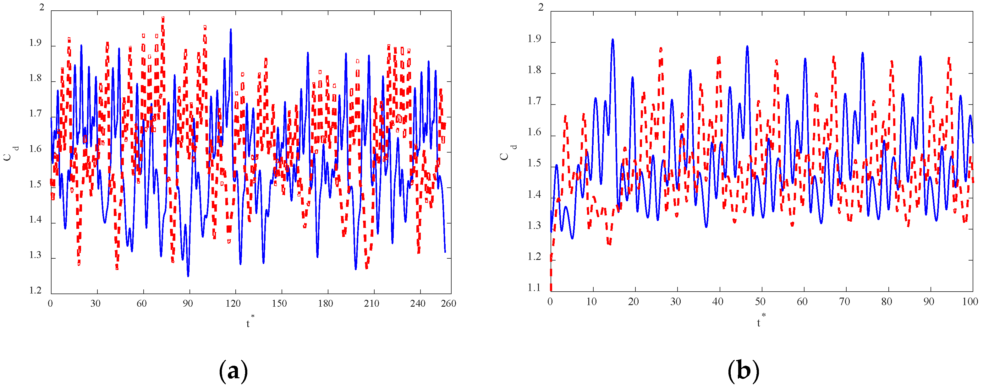
Figure 4a–c show the instantaneous drag time-trace, Cd, for each cylinder at Red = 200, 1000, and 3000, respectively. The mean average drag can be computed from each time history signal.
Vu et al. [33] suggested that the mean average drag coefficient should be computed as an equivalent drag, .
The computation would be based on each cylinder and compared to a single circular cylinder under the same Reynolds number, , remembering that the time average processes were carried out over the total transient simulation.
Following Equation (9), the equivalent was found to be 1.20, 1.33, and 2.16 for the Reynolds numbers 200, 1000, and 3000, respectively. These results are in good agreement with the results from Vu et al. [33], mainly for the cases at Red = 200 and 1000. In their paper, the authors simulated 2D flow around circular cylinders in pairs under the same Reynolds numbers and p/d ratio. The equivalent drag, , was found to differ from ours by only 0.6% under Red = 200 and no difference was found under Red = 1000. Unfortunately, the same computation methodology could not be applied to Afgan’s results in order to compare the outcomes for Red = 3000, since the authors evaluated the Cd based on the wakes’ topologies. However, Afgan et al. [27] state that the sum of the drag coefficients of the two cylinders, separately, is slightly comparable to twice the drag found in a single circular cylinder for 1.25 ≤ p/d ≤ 5.0. By carefully observing the data published by the authors, the total drag was found to be 2.80. Applying this methodology using = yielded a value of 2.89, which differs by only 3.2% from Afgan’s results [2].
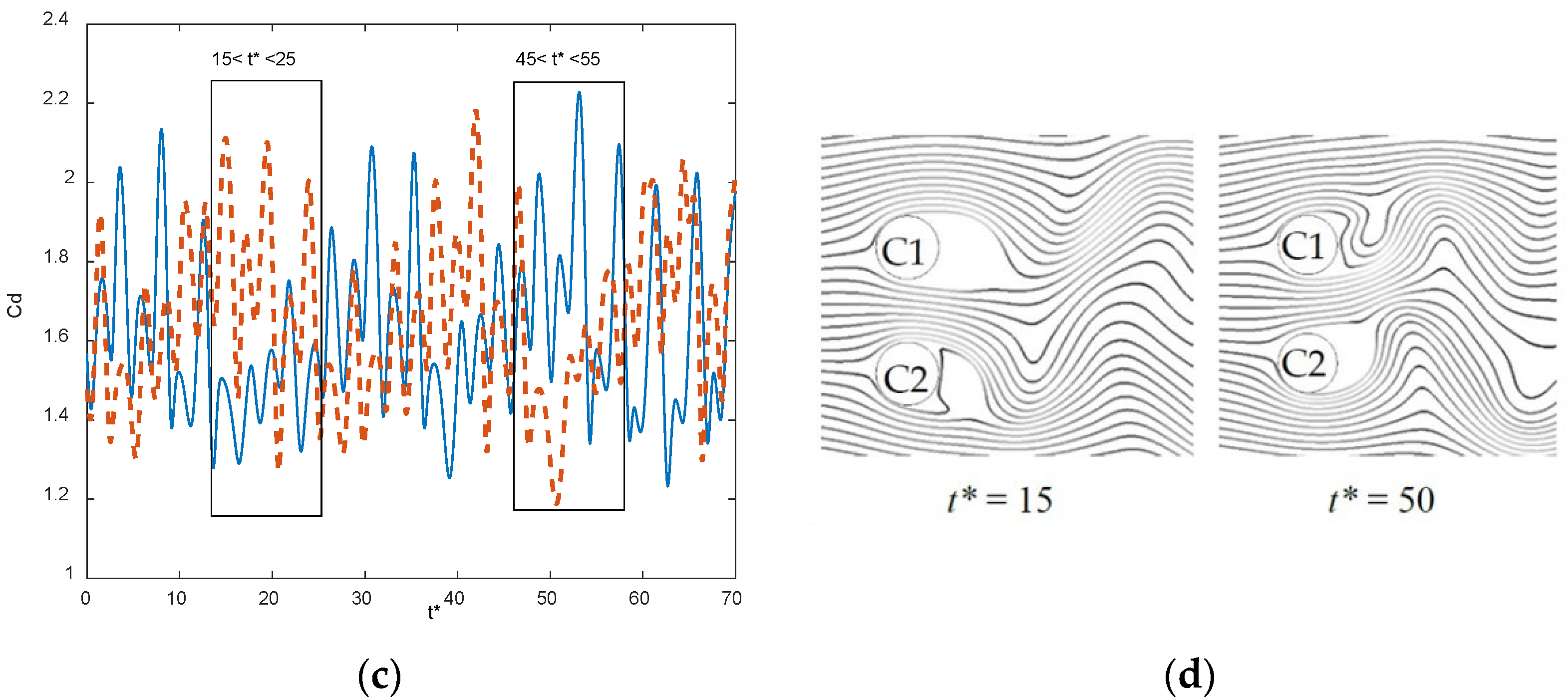
The bistable flow process was also a target of our research. The bistability phenomenon takes place when the wakes are near enough to interact to each other. This interaction yields stable modes of wake topologies that change randomly over time. During the processes, a narrow and wide wake is formed behind each cylinder. In the first moment, a wide wake behind the lower cylinder moves out behind the upper cylinder, whose wake is narrow at first. This switching occurs over time and each mode lasts for a certain period of time [18,19]. Stable modes are observed in all cases. However, in the third case, Red = 3000, the observation is straightforward. Figure 4d shows the instantaneous streamlines over the cylinders corresponding to the times t* = 15 and t* = 50 for the case of Red = 3000. From the picture, it is possible to observe that the wake topology is stable for a certain period of time behind each cylinder (see the rectangles in Figure 4c). As previously stated, the direction of the central jet determines which cylinder will experience either the narrow wake (NW) or the wide one (WW), thus ruling the drag coefficient on each cylinder.
In fact, by observing the drag time-traces in each cylinder, higher and lower drag coefficients are assigned to different wakes’ topologies. See the first stable mode at 15 ≤ t* ≤ 25 in Figure 4c. In this moment, we can identify that the lower cylinder, C2, experiences a higher value of drag and, at once, the viscous wake behind it is classified as a narrow wake (NW; Figure 4d). On the other hand, when the new topology takes place, from t* ~ 45 to 55, the drag value in the upper cylinder is higher than that found in the lower one. Again, Figure 4d identifies the narrow wake (NW) downstream of the upper cylinder, leading to a high drag value. The dependence of the drag force on the stable wake topologies has been pointed out by several authors [14,20,33]. During the time that the lower cylinder experiences the narrow wake, the mean average drag is computed differently; is 1.60 and is 1.30. According to Alam et al. [20], the drag coefficient difference between the narrow wake and the wider one is due to the pressure recovery behind each wake.
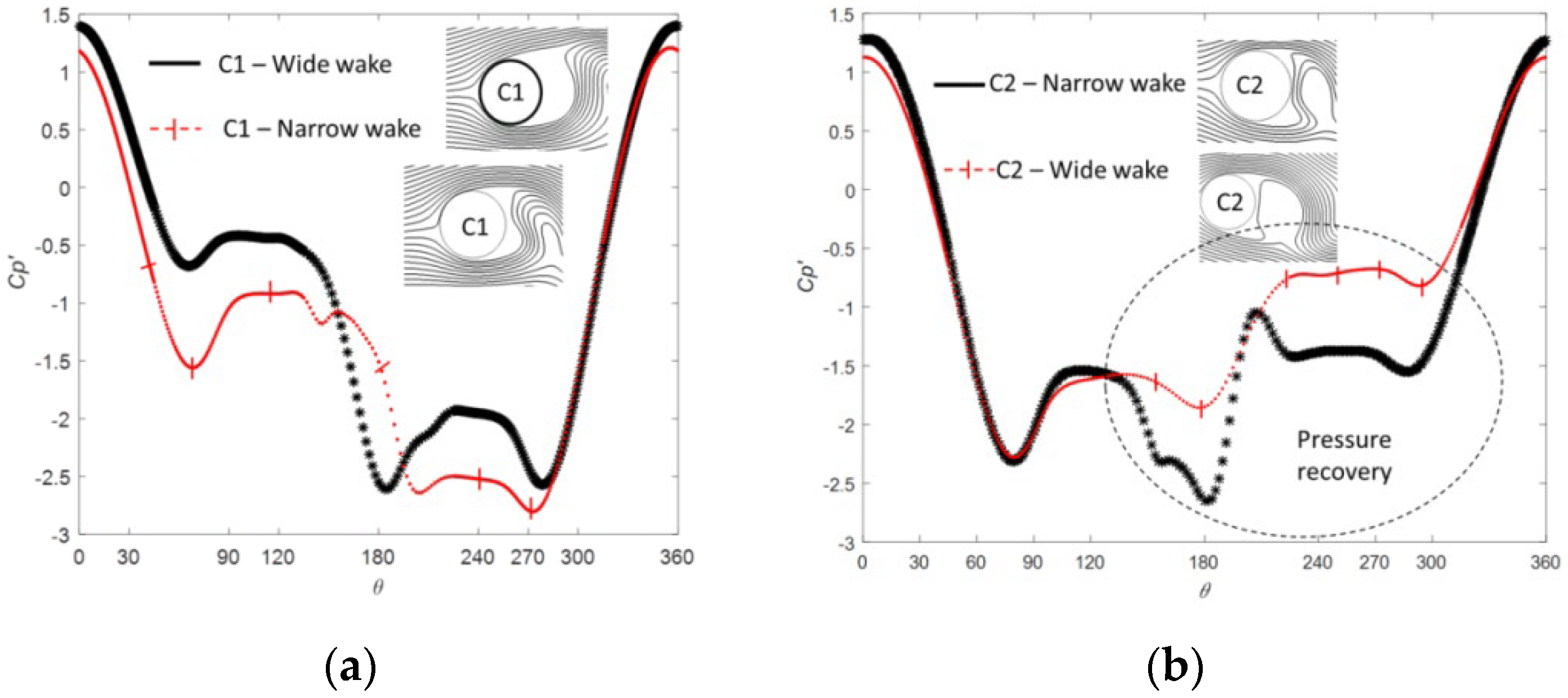
The instantaneous pressure distribution, Cp′, around each cylinder was also investigated. Figure 5a,b intend to show the instantaneous pressure distribution around the same cylinders in each stable mode. This information may help us to understand how the drag coefficient is associated with the wake topology, since in blunt bodies, the pressure (or shape) drag is expected to play a major role in the total drag [34].
In both pictures, the same cylinder is seen to experience almost the same pressure distribution at the very beginning, regardless of the wake topology behind them. After some angular positions, towards the rear part of the cylinders, the curves reveal different pressures. This behavior is seen to happen for the upper cylinder from θ ~ 40° to 270°, while on the lower cylinder’s surface, the same behavior appears soon after θ = 120° up to 320°. However, the most important part of the graph is the middle part. The reader can easily see that the pressure recovery is different for the same cylinder under the different modes (wake topologies). The upper cylinder, under the wide wake (WW), experiences higher levels of pressure in its front and rear part as well. On the other hand, when the mode switches and, therefore, the same cylinder is under the narrow wake (NW), the pressure is lowered in the same position in comparison with what would be under the other mode (Figure 5a). The same analogy can be employed for the lower cylinder, C2. In this case, the differences between the levels of pressure are even larger. Furthermore, we can also easily observe the pressure recovery behind the cylinder subject to the wide wake (WW), indicating that the instantaneous shape drag should be lowered in comparison with the same cylinder in NW mode (Figure 5b).
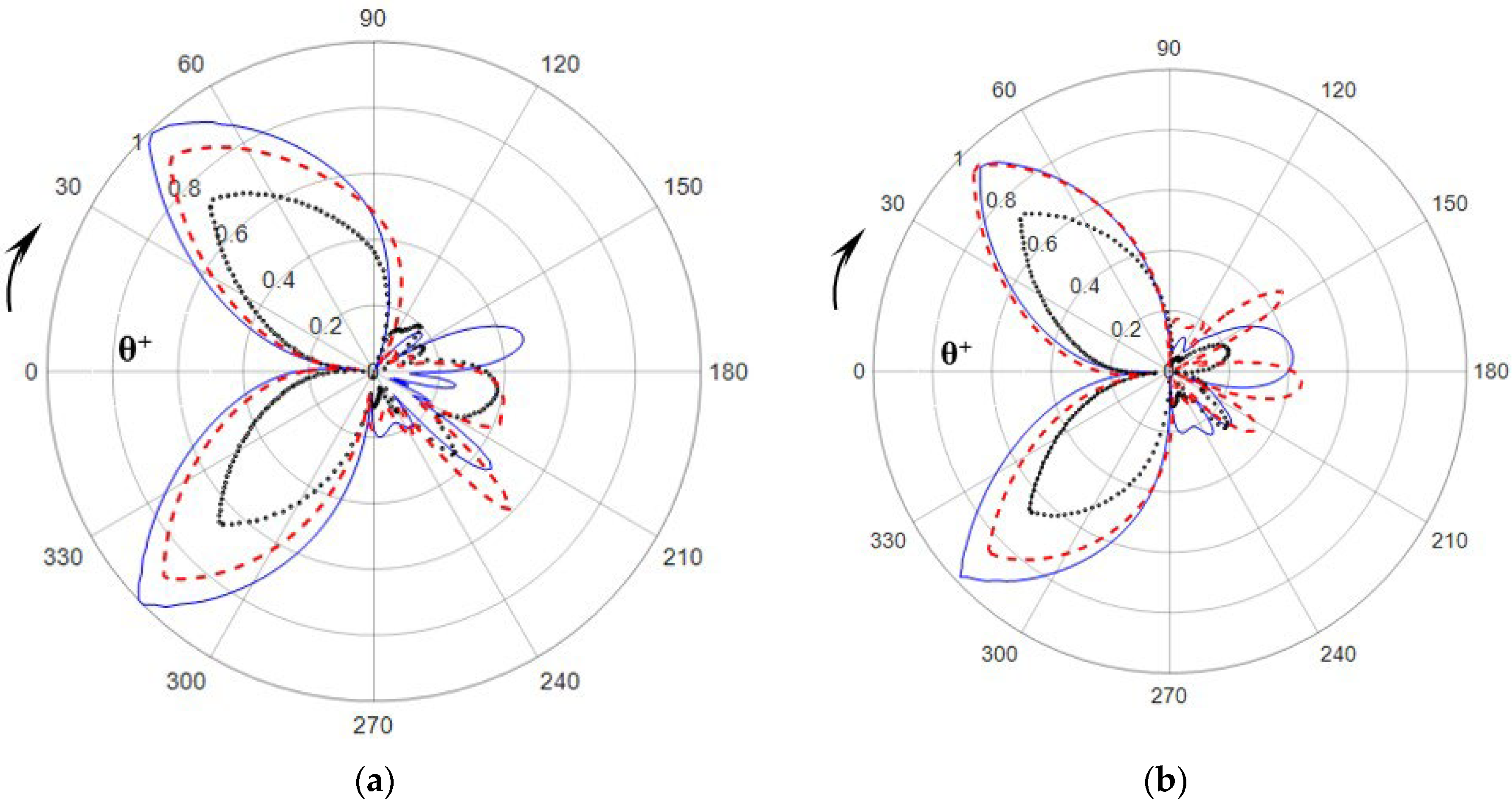
Velocity time-traces were gathered at the monitoring point (Figure 1b), at once. The time, t*, was made dimensionless, as mentioned before, and the velocity component received the same treatment by using the free stream velocity, U∞, as follows:
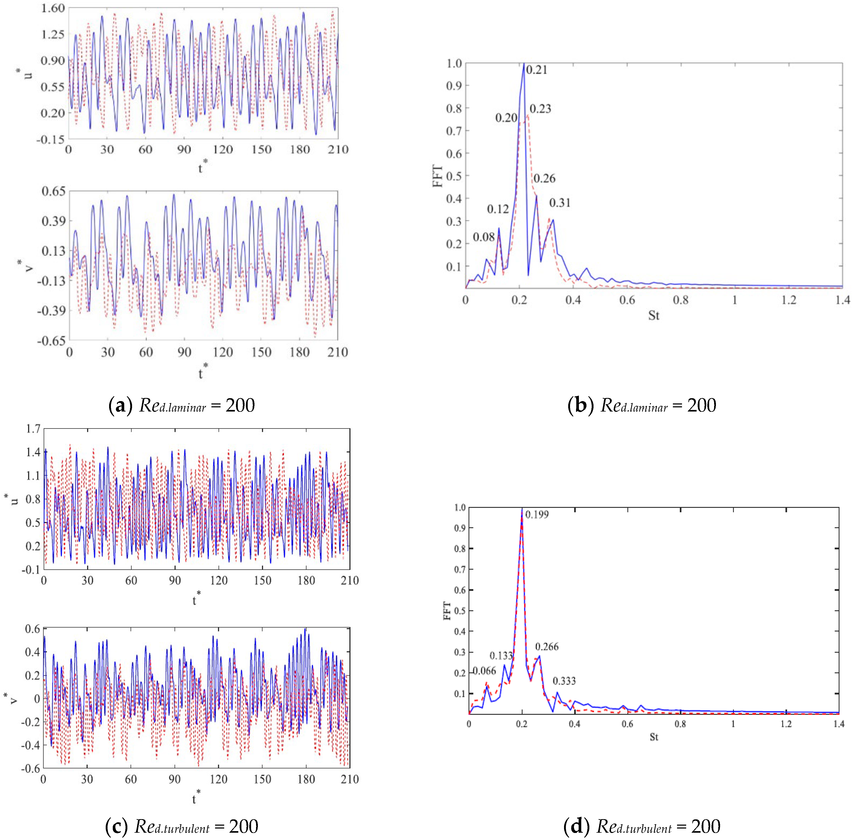
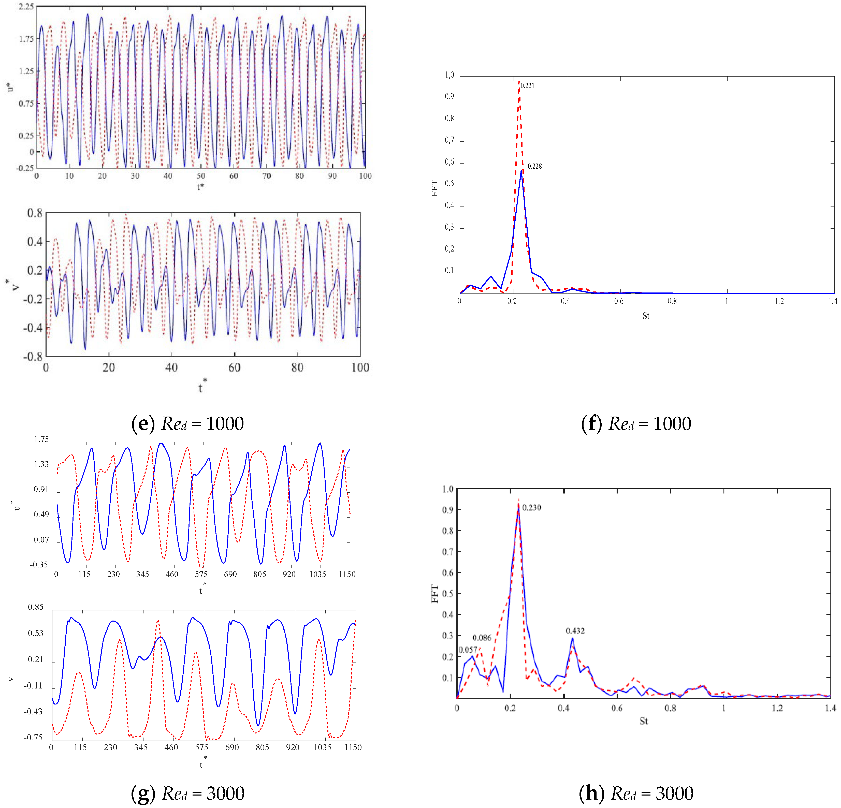
where u and v are the axial and transversal instantaneous velocities. We also carried out numerical simulations for the lowest Red case without any turbulence model (laminar flow). In this case, we want to investigate whether the employed turbulence model affects somehow the spectral response of the flow field. The fast Fourier transform (FFT) employed here was performed using 2N data point for each velocity time-trace signal (N is the number of data on each signal). Before performing the FFT computations, the signals were windowed by a Hanning function. The FFT coefficients were scaled by the highest one. By observing the velocity signals in the wakes, one can see that the flow exhibits almost periodic patterns, mainly for higher Reynolds numbers. The Fourier transform coefficients of each signal are plotted along with the velocity time-traces (Figure 6b,d,f,h). The frequency was then made dimensionless through the Strouhal number as follows:
where is the main frequency in the spectrum in Hz.
The dynamics of the flow were found to be in fair agreement with Bearman’s findings [15]. As predicted by the authors [15], the cylinders are far enough apart to maintain a fundamental frequency very close to what one would expect in a single cylinder. In fact, the spectral analysis has shown that the fundamental frequency peak appears at about St ~ 0.20. A slight displacement towards higher frequencies is seen as the Reynolds number increases. Moreover, both velocity components presented the same frequencies. It should also be pointed out that the spectral response of the flow seems to be unaffected by the turbulence model. Both spectra for laminar and turbulent flow at Red = 200 showed almost the same fundamental peak at St ~ 0.20. Several peaks, besides the fundamental one, appear for each Reynolds number simulated, indicating that the biased flow deflection, i.e., the bistable flow, exists and possesses its very own signature in terms of spectral response. Indeed, such a feature was successfully seen in the Cd time-traces (Figure 4a–c).
Afgan and his co-workers [27] investigated the power spectral response of the flow dynamics for several p/d ratios under the same Reynolds number, 3000. For p/d < 2.0, the authors identified different peaks in the spectra; however, as the gap increased, the additional peaks vanished. In the same year, similar results were released by Verna and Verna and Govardhan [35], who investigated 2-D flow over side-by-side circular cylinders. Both works from 2011 [27,35] connect the secondary frequencies to different wake topologies, and lower frequency was assigned to the wide wake (WW); on the other hand, the higher one was related to the narrow wake (NW). Afgan and co-workers [27] associated the Strouhal numbers St ~ 0.11 and 0.39 to the wide wake (WW) and narrow wake (NW), respectively, for a p/d ratio 1.50; on the other hand, according to the authors, for p/d = 2.0, the peaks in the spectra were seen to be very close. Sided peaks, at distinguished frequencies, were also reported by Pang et al. [36] and Alam et al. [20]. In the former work, the authors studied the dynamical response of the flow field in a 2D domain under the Reynolds number 60,000 for several p/d ratios. The authors [36] associated a Strouhal number of 0.10 to the wide wake (WW) and the narrow wake (NW) was assigned to the Strouhal 0.3. Furthermore, intermediated frequencies, at St ~0.2, were found for 1.1≤ p/d ≤ 2.6.
In Figure 6h, the reader can see that the Strouhal numbers are about 0.06 and 0.43, indicating dimensionless frequencies for different wake topologies. Higher frequency was associated with the narrow wake (NW) and vice versa.
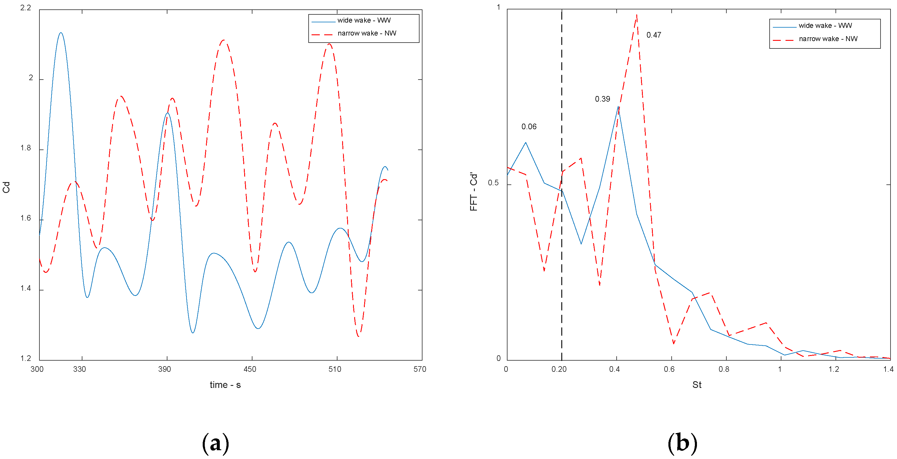
In order to promote a better understanding of the wakes’ characteristic frequency, the spectral response of the Cd signal, at Red = 3000, was analysed. Since we have very distinctive patterns of Cd, assigned to different wakes’ topologies, the drag signal was split into Cd–narrow wake and Cd–wide wake. Figure 7a,b show both the Cd time-trace and the fast Fourier transform of those signals. From Figure 7b, one can observe that the spectral response of each wake topology is different. The wide wake (WW) stresses lower frequencies in comparison with the narrow wake (NW). The WW exhibits its main Fourier coefficients at St = 0.06 and 0.39, whereas for the NW, the most important coefficients are assigned to the fundamental frequency at about St = 0.47.
4. Concluding Remarks
Isothermal, 2-D, and incompressible turbulent flow over a pair of circular cylinders arranged side-by-side was investigated by numerical simulation in this work. The main dimensionless number that qualified the simulation was the pitch–diameter ratio, p/d, which was kept constant at 2 throughout the work. In order to quantify the Reynolds effects, three Reynolds numbers were also simulated by varying the entrance velocity. The computations were carried out on a finite-volumes platform using Unsteady RANS-k-ω SST to overcome the closure problem of the turbulence.
The stagnation and detachment angles of the boundary layer were measured. The simulations were in quite good agreement when compared with the results reported by other authors. The Reynolds numbers were found to play a more important role in the stagnation angle, θEST, than the detached one, δSEP, for any case simulated.
The mean and time history drag coefficients were also gathered. Asymmetric and irregular behavior of the drag coefficients was observed regardless of the Reynolds number. Furthermore, different wake topologies were formed behind the cylinders, causing the cylinders to experience different drag forces. The instantaneous drag force was seen as a function of the type of wake topology formed behind each one. Higher drag was assigned to narrow wakes (NW) and lower drags were seen to be related to wide wakes (WW). Furthermore, the instantaneous Cp′ around the cylinder, under different wake topologies, showed that the pressure recovers behind them when they are in the wide wake mode (WW); otherwise, the pressure is lowered, enhancing the drag force for the narrow wake mode (NW).
The Reynolds number seems to work in order to delay the changes between the wake topologies. As the Reynolds number increases, each wake topology lasts longer. In other words, as the Reynolds number increases, the number of changes experienced by each cylinder seems to decrease.
The spectral-flow response was also analyzed through the velocity time-traces behind the structures. A very well-distinguished peak was found in the spectrum at St ~ 0.20, which is in fair agreement with other research. A slight displacement towards higher frequencies could be seen as the Reynolds number increased, but it was marginal. Secondary peaks located on either of the main peaks in the spectrum were also observed, mainly for Reynolds numbers of 200 and 3000. The marginal peaks are associated with the different wake topologies behind the cylinders. The lower and higher frequency could be very well associated with the wakes through the spectral response of the Cd time-traces. In the narrow wake mode, which produced a higher Cd yield, high Fourier coefficients placed at higher frequencies, whereas for the wide wake, the higher Fourier coefficients were assigned to the lower frequencies.
The laminar simulations, Red = 200 (without any turbulence model), did not show any difference in the dynamics of the fluctuant flow field. This result shows that the employed turbulence model neither affects nor fosters the bistable flow mode in the pair of cylinders studied.
Author Contributions
Conceptualization, T.G. and J.G.; Funding acquisition, J.G.; Investigation, T.G.; Methodology, T.G. and C.A.; Project administration, J.G.; Resources, C.A. and J.G.; Software and Data treatment, T.G. and J.G.; Validation, C.A. and J.G. Writing—original draft, T.G.; Writing—review and editing, C.A. and J.G. All authors have read and agreed to the published version of the manuscript.
Funding
This research received no external funding.
Informed Consent Statement
Not applicable.
Data Availability Statement
Not applicable.
Acknowledgments
The first author would like to thank the Coordenação de Aperfeiçoamento de Pessoal de Nível Superior-Brasil (CAPES)-Finance Code 001 for supporting him during this research with a fellowship. The second author thanks CNPQ and FAPDF for supporting him with financial resources through the projects n° 193.001.158/2015, 193.001356/2016 and 408869/2016-0.
Conflicts of Interest
The authors declare no conflict of interest.
References
- Grimison, E.D. Correlation and Utilization of New Data on Flow Resistence and Heat Transfer for Cross Flow of Gases Over Tube Banks; Transactions: Process Industries Division; American Society of Mechanical Engineers: New York, NY, USA, 1937; pp. 583–594. [Google Scholar]
- Wiemer, P. Untersuchung Über den Zugwiederstand Von Wasserrohrkesseln, Dissertation; RWTH: Aachen, Germany, 1937. [Google Scholar]
- Žukauskas, A.A. Heat transfer from tubes in crossflow. In Advances in Heat Transfer; Elsevier: Amsterdam, The Netherlands, 1972; Volume 8, pp. 93–160. [Google Scholar]
- Žukauskas, A.A.; Katinas, V.J.; Perednis, E.E.; Sobolev, V.A. Viscous flow over inclined in-line tube bundles, and vibrations induced in the latter. Fluid Mech. Sov. Res. 1980, 9, 1–12. [Google Scholar]
- Žukauskas, A.A.; Katinas, V.J. Fluid Dynamics forces on vibrating tubes of heat exchangers in cross flow. In International Symposium on Flow-Induced Vibration and Noise; ASME: Chicago, IL, USA, 1988; Volume 1, pp. 127–142. [Google Scholar]
- Derakhshandeh, J.F.; Alam, M.M. A review of bluff body wakes. Ocean Eng. 2019, 182, 475–488. [Google Scholar] [CrossRef]
- Zdravkocich, M.M.; Pridden, D.L. Interference between two circular cylinders; series of unexpected discontinuities. J. Ind. Aerodyn. 1977, 2, 255–270. [Google Scholar] [CrossRef]
- Young, E.W.K.; Martinex, D.M.; Olso, J.A. The sedimentation of papermaking fibers. Am. Inst. Chem. Eng. 2006, 52, 2697–2706. [Google Scholar] [CrossRef]
- Ahmad, N.; Bihs, H.; Myrhaug, D.; Kamath, A.; Arntsen, O.A. Three-dimensional numerical modelling of wave-induced scour around piles in a side-by-side arrangement. Coast. Eng. 2018, 138, 132–151. [Google Scholar] [CrossRef]
- Alam, M.; Zhou, Y. Flow around two side-by-side closely spaced circular cylinders. J. Fluids Struct. 2007, 23, 799–805. [Google Scholar] [CrossRef]
- Alam, M.; Zheng, Q.; Hourigan, K. The wake and thrust by four side-by-side cylinders at a low Re. J. Fluids Struct. 2017, 70, 131–144. [Google Scholar] [CrossRef]
- Kim, S.; Alam, M.M. Characteristics and suppression of flow-induced vibrations of two side-by-side circular cylinders. J. Fluids Struct. 2015, 54, 629–642. [Google Scholar] [CrossRef]
- Shao, J.; Zhang, C. Large eddy simulations of the flow past two side-by-side circular cylinders. Int. J. Comput. Fluid Dyn. 2008, 22, 393–404. [Google Scholar] [CrossRef]
- Sumner, D. Two circular cylinders in cross-flow: A review. J. Fluids Struct. 2010, 26, 849–899. [Google Scholar] [CrossRef]
- Bearman, P.W.; Wadcok, A.J. The interaction between a pair for circular cylinders normal to a stream. J. Fluid Mech. 1973, 61, 499–511. [Google Scholar] [CrossRef]
- Meneghini, J.R.; Saltara, F.; Siqueira, C.; Ferrari, J. Numerical Simulation of Flow Interference between Two Circular Cylinders in Tandem and Side-by-Side Arrangements. J. Fluids Struct. 2001, 15, 327–350. [Google Scholar] [CrossRef]
- Olinto, C.R.; Indrusiak, M.L.S.; Endres, L.A.M.; Möller, S.V. Experimental study of the characteristics of the flow in the first rows of tube banks. Nucl. Eng. Des. 2009, 239, 2022–2034. [Google Scholar] [CrossRef]
- De Paula, A.V.; Endres, L.A.M.; Möller, S.V. Experimental study of the bistability in the wake behind three cylinders in triangular arrangement. J. Braz. Soc. Mech. Sci. Eng. 2013, 35, 163–176. [Google Scholar] [CrossRef]
- Neumeister, R.F.; Petry, A.P.; Möller, S.V. Characteristics of the wake formation and force distribution of the bistable flow on two cylinders side-by-side. J. Braz. Soc. Mech. Sci. Eng. 2018, 40, 564. [Google Scholar] [CrossRef]
- Alam, M.; Moriya, M.; Sakamoto, H. Aerodynamic characteristics of two side-by-side circular cylinders and application of wavelet analysis on the switching phenomenon. J. Fluids Struct. 2003, 18, 325–346. [Google Scholar] [CrossRef]
- Giacomello, M.V.; Rocha, L.A.; Schettini, E.B.; Silvestrini, J.H. Simulação numérica de escoamentos ao redor de cilindros com tranferência de calor. In Anais da 5ª Escola de Primevera de Transição e Turbulência; EPTT: Rio de Janeiro, Brasil, 2006; pp. 25–30. [Google Scholar]
- Kang, S. Characteristics of flow over two circular cylinders in a side-by-side arrangement at low Reynolds numbers. Phys. Fluid 2003, 15, 712–714. [Google Scholar] [CrossRef]
- Wang, Z.; Zhou, Y. Vortex interactions in a two side-by-side cylinder near-wake. Int. J. Heat Fluid Flow 2005, 26, 362–377. [Google Scholar] [CrossRef]
- Vila, J.L.; Gomes, T.F.; De Melo, T.; Goulart, J.N.V. Experimental measurements of pressure and velocity fields around circular cylinders arranged in pair. In Proceedings of the 25th International Congress of Mechanical Engineering—COBEM, Uberlândia, Brazil, 20–25 October 2019. [Google Scholar]
- Chen, W.; Ji, C.; Xu, D.; Srinil, N. Wake patterns of freely vibrating side-by-side circular cylinders in laminar flows. J. Fluids Struct. 2019, 89, 82–95. [Google Scholar] [CrossRef]
- Chen, W.; Ji, C.; Xu, D.; An, H.; Zhang, Z. Flow-induced vibrations of two side-by-side circular cylinders at low Reynolds numbers. Phys. Fluids 2020, 32, 023601. [Google Scholar] [CrossRef]
- Afgan, I.; Kahil, Y.; Benhamadouche, S.; Sagaut, P. Large eddy simulation of the flow around single and two side-by-side cylinders at subcritical Reynolds numbers. Phys. Fluids 2011, 23, 075101. [Google Scholar] [CrossRef]
- Menter, F.R. Two-equation eddy-viscosity turbulence models for engineering applications. AIAA J. 1994, 32, 1598–1605. [Google Scholar] [CrossRef]
- Candela, D.S.; Gomes, T.F.; Goulart, J.; Anflor, C.T.M. Numerical simulation of turbulent flow in an eccentric channel. Eur. J. Mech. B/Fluids 2020, 83, 86–98. [Google Scholar] [CrossRef]
- Goulart, J.; Wissink, J.G.; Wrobel, L.C. Numerical simulation of turbulent flow in a channel containing a small slot. Int. J. Heat Fluid Flow 2016, 61, 343–354. [Google Scholar] [CrossRef]
- Achenbach, E. Distribution of local pressure and skin friction around a circular cylinder in cross-flow up to Re = 5 × 10⁶. J. Fluid Mech. 1968, 34, 625–639. [Google Scholar] [CrossRef]
- Hensan, S.M.; Navid, N. Numerical simulation of flow over two side-by-side circular cylinders. J. Hydrodyn. 2011, 23, 792–805. [Google Scholar]
- Vu, H.C.; Ahn, J.; Hwang, J.H. Numerical simulation of flow past two circular cylinders in tandem and side-by-side arrangement at low Reynolds numbers. KSCE J. Civ. Eng. 2015, 20, 1594–1604. [Google Scholar] [CrossRef]
- White, F.M. Fluid Mchanics, 4th ed.; MacGraw-Hill: New York, NY, USA, 1999. [Google Scholar]
- Verma, P.L.; Govardhan, M. Flow behind bluff bodies inf side-by-side arrangement. J. Eng. Sci. Technol. 2011, 6, 745–768. [Google Scholar]
- Pang, J.H.; Zong, Z.; Zou, L.; Wang, Z. Numerical simulation of the flow around two side-by-side circular cylinders by IVCBC vortex method. Ocean. Eng. 2016, 119, 86–100. [Google Scholar] [CrossRef]
Figure 1.
(a) Schematic view of the domain. (b) Probes’ location.

Figure 2.
Nondimensional wall distance, y+, for cylinders’ surfaces at Red = 3000. (a) Upper cylinder. (b) Lower cylinder―Mesh 1 (coarse); Mesh 2 (medium); o Mesh 3 (fine).
Figure 2.
Nondimensional wall distance, y+, for cylinders’ surfaces at Red = 3000. (a) Upper cylinder. (b) Lower cylinder―Mesh 1 (coarse); Mesh 2 (medium); o Mesh 3 (fine).

Figure 3.
Mean average pressure skin friction coefficients as a function of the angular position. (a) Cp distribution for the upper. (b) Cp distribution for the lower cylinder. (c) Skin friction distribution for the upper cylinder. (d) Skin friction distribution for the upper cylinder. ―Red. = 200; +++ Red = 1000 and °°° Red = 3000.

Figure 4.
Instantaneous drag coefficients’ time history. (a) Reynolds 200. (b) Reynolds 1000. (c) Reynolds 3000. (d) Stable modes of wakes—narrow and wide wakes formation for different t*, under Red = 3000. ― Upper cylinder. - - - Lower cylinder.
Figure 4.
Instantaneous drag coefficients’ time history. (a) Reynolds 200. (b) Reynolds 1000. (c) Reynolds 3000. (d) Stable modes of wakes—narrow and wide wakes formation for different t*, under Red = 3000. ― Upper cylinder. - - - Lower cylinder.


Figure 5.
Instantaneous pressure coefficient around the cylinders at Red = 3000. (a) Upper cylinder (C1) experiencing two different modes. (b) Lower cylinder (C2) experiencing two different modes.
Figure 5.
Instantaneous pressure coefficient around the cylinders at Red = 3000. (a) Upper cylinder (C1) experiencing two different modes. (b) Lower cylinder (C2) experiencing two different modes.

Figure 6.
Time-traces of velocity components in the wake for upper and lower cylinders, along with the spectral computation of the flow velocity signal. ― Upper cylinder. - - - Lower cylinder.
Figure 6.
Time-traces of velocity components in the wake for upper and lower cylinders, along with the spectral computation of the flow velocity signal. ― Upper cylinder. - - - Lower cylinder.


Figure 7.
(a) Cd time-traces for different wakes. (b) spectral computation of the flow Cd signal. ___ wide wake (WW). - - - narrow wake (NW).
Figure 7.
(a) Cd time-traces for different wakes. (b) spectral computation of the flow Cd signal. ___ wide wake (WW). - - - narrow wake (NW).


Table 1.
Mesh characteristic. The stagnation, θEst, and separation angles, δSep, for Red = 3000 and p/d ratio 2.0.
Table 1.
Mesh characteristic. The stagnation, θEst, and separation angles, δSep, for Red = 3000 and p/d ratio 2.0.
| θEst Upper | θEst Lower | δSep Upper | δSep Lower | Total Nodes | N° Divisions on Cylinders’ Surfaces | |||
|---|---|---|---|---|---|---|---|---|
| Afgan et al., 2011 | 353.7 | 8.1 | 83.8 | 262.1 | 99.8 | 276.3 | ---------- | ---------- |
| Mesh 1 | 353.6 | 7.7 | 87.0 | 265.7 | 104.9 | 278.1 | 216,000 | 492 |
| Mesh 2 | 353.6 | 7.7 | 85.5 | 263.5 | 101.7 | 277.3 | 235,000 | 504 |
| Mesh 3 | 353.6 | 7.7 | 84.9 | 262.8 | 100.2 | 276.4 | 241,000 | 504 |
Table 2.
Stagnation and separation angles for each cylinder as a function of Reynolds number.
| Red | θEst Upper | θEst Lower | δSep Upper | δSep Lower | ||
|---|---|---|---|---|---|---|
| 200 | 351.20 | 9.30 | 82.20 | 246.50 | 97.90 | 252.60 |
| 1000 | 352.50 | 8.80 | 84.40 | 262.30 | 99.50 | 263.30 |
| 3000 | 353.60 | 7.70 | 85.50 | 263.50 | 101.70 | 277.30 |
Publisher’s Note: MDPI stays neutral with regard to jurisdictional claims in published maps and institutional affiliations. |
© 2022 by the authors. Licensee MDPI, Basel, Switzerland. This article is an open access article distributed under the terms and conditions of the Creative Commons Attribution (CC BY) license (https://creativecommons.org/licenses/by/4.0/).
Share and Cite
MDPI and ACS Style
Gomes, T.; Goulart, J.; Anflor, C. Hydrodynamic Characteristics of Two Side-by-Side Cylinders at a Pitch Ratio of 2 at Low Subcritical Reynolds Numbers. Fluids 2022, 7, 287. https://0-doi-org.brum.beds.ac.uk/10.3390/fluids7090287
AMA Style
Gomes T, Goulart J, Anflor C. Hydrodynamic Characteristics of Two Side-by-Side Cylinders at a Pitch Ratio of 2 at Low Subcritical Reynolds Numbers. Fluids. 2022; 7(9):287. https://0-doi-org.brum.beds.ac.uk/10.3390/fluids7090287
Chicago/Turabian StyleGomes, Thiago, Jhon Goulart, and Carla Anflor. 2022. "Hydrodynamic Characteristics of Two Side-by-Side Cylinders at a Pitch Ratio of 2 at Low Subcritical Reynolds Numbers" Fluids 7, no. 9: 287. https://0-doi-org.brum.beds.ac.uk/10.3390/fluids7090287