
From Navier to Stokes: Commemorating the Bicentenary of Navier’s Equation on the Lay of Fluid Motion

1
Department of Civil Engineering, University of Chile, Santiago 8370448, Chile
2
Advanced Mining Technology Center, University of Chile, Santiago 8370448, Chile
Fluids 2024, 9(1), 15; https://0-doi-org.brum.beds.ac.uk/10.3390/fluids9010015
Submission received: 7 November 2023
/
Revised: 21 December 2023
/
Accepted: 30 December 2023
/
Published: 6 January 2024
(This article belongs to the Topic Fluid Mechanics)
Abstract
:The article presents a summarised history of the equations governing fluid motion, known as the Navier–Stokes equations. It starts with the work of Castelli, who established the continuity equation in 1628. The determination of fluid flow resistance was a topic that involved the brightest minds of the 17th and 18th centuries. Navier’s contribution consisted of the incorporation of molecular attraction effects into Euler’s equation, giving rise to an additional term associated with resistance. However, his analysis was not the only one. This continued until 1850, when Stokes firmly established the boundary conditions that must be applied to the differential equations of motion, specifically stating the non-slip condition of the fluid in contact with a solid surface. With this article, the author wants to commemorate the bicentennial of the publication of “Sur les Lois du Mouvement des Fluides” by Navier in the Mémoires de l’Académie Royale des Sciences de l’Institut de France.
1. Introduction
This year marks the 200th anniversary since the article “Sur les Lois du Mouvement des Fluides” by Claude Louis Marie Henri Navier was published in the Mémoires de l’Académie Royale des Sciences de l’Institut de France. As Navier’s work is part of the foundations of fluid mechanics, the author considers it appropriate to commemorate it in a journal devoted to fluids and their motion. This article presents a summary of Navier’s contribution to the controversial problem of fluid resistance to motion, which engaged the brightest minds in mathematics, physics, and engineering from the 18th until the mid-19th centuries, when the work of Stokes definitively consolidated what we now identify as the Navier–Stokes equations.
Before presenting how Navier introduced the resistance of motion, it is interesting to mention some of his biography, taken from McKeon (1981) [1]. Navier was born in Dijon on 10 February 1785, and died on 21 August 1836, in Paris. His father was a lawyer for the Legislative Assembly in Paris during the French Revolution and died in 1793, leaving him under the guardianship of his great-uncle Emiland Gauthey, chief engineer of the Corps of Bridges and Roads of Paris, who educated and prepared him to enter the École Polytechnique in 1802, where he had Joseph Fourier as professor of analysis (calculus), who would become his protector and later, friend. In 1804, Navier entered the École des Ponts et Chaussées, graduating in 1806. It is important to mention Navier’s passage through both schools: In the first, he acquired a rigorous mathematical and theoretical education, while in the second, he received an orientation to the practice of engineering. Navier would know how to take advantage of this complementary education. A few months after his graduation, his great-uncle passed away, and the administration of the Corps of Bridges and Roads commissioned Navier in 1807 to edit Gauthey’s manuscripts, which were published between 1809 and 1816. From 1819, Navier oversaw the applied mechanics courses at the École des Ponts et Chaussées. In parallel with the edition of his great-uncle’s engineering manuscripts, from 1807 to 1820, he made mathematical analysis a fundamental tool of civil engineering. The combination of these two skills, theoretical-analytical and practical application to engineering, was fundamental to the contributions he made in solid mechanics (elasticity) and fluid mechanics [2].
2. The Problem of the Motion of Fluids
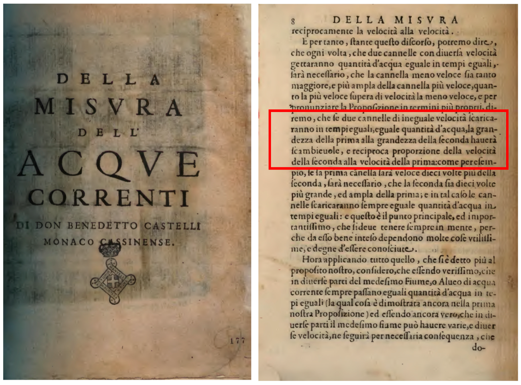
Arbitrarily, and just to establish a starting point, we can say that modern hydraulics began as an experimental science in Italy in the 16th century, becoming more theoretical in the following century. Benedetto Castelli (c.1577–c.1644) is one of its best exponents by presenting the equation of continuity in his treatise Della misura delle acque correnti in 1628. Although the propositions established by Castelli in his treatise had already been indicated by Leonardo da Vinci a century earlier, he did not divulge them, so they remained unknown until the codices with his works began to be rediscovered and known. Leonardo did not form disciples, unlike Galileo Galilei, who was able to form a school, with Benedetto Castelli being one of his most accomplished students. The continuity equation for a steady-state regime is stated on page 8 of the 1639 edition of the book that the author had access to [3], and it is shown in the lines within the rectangle in Figure 1. A loose translation of the text is “if two pipes with unequal velocity in the same amount of time, discharge the same amount of water, the size of the first to the size of the second will have a reciprocal proportion to the velocity of the second to the velocity of the first”. That is, if the flow discharged in two pipes is the same, then , with the subindexes 1 and 2 denoting each of the conduits.
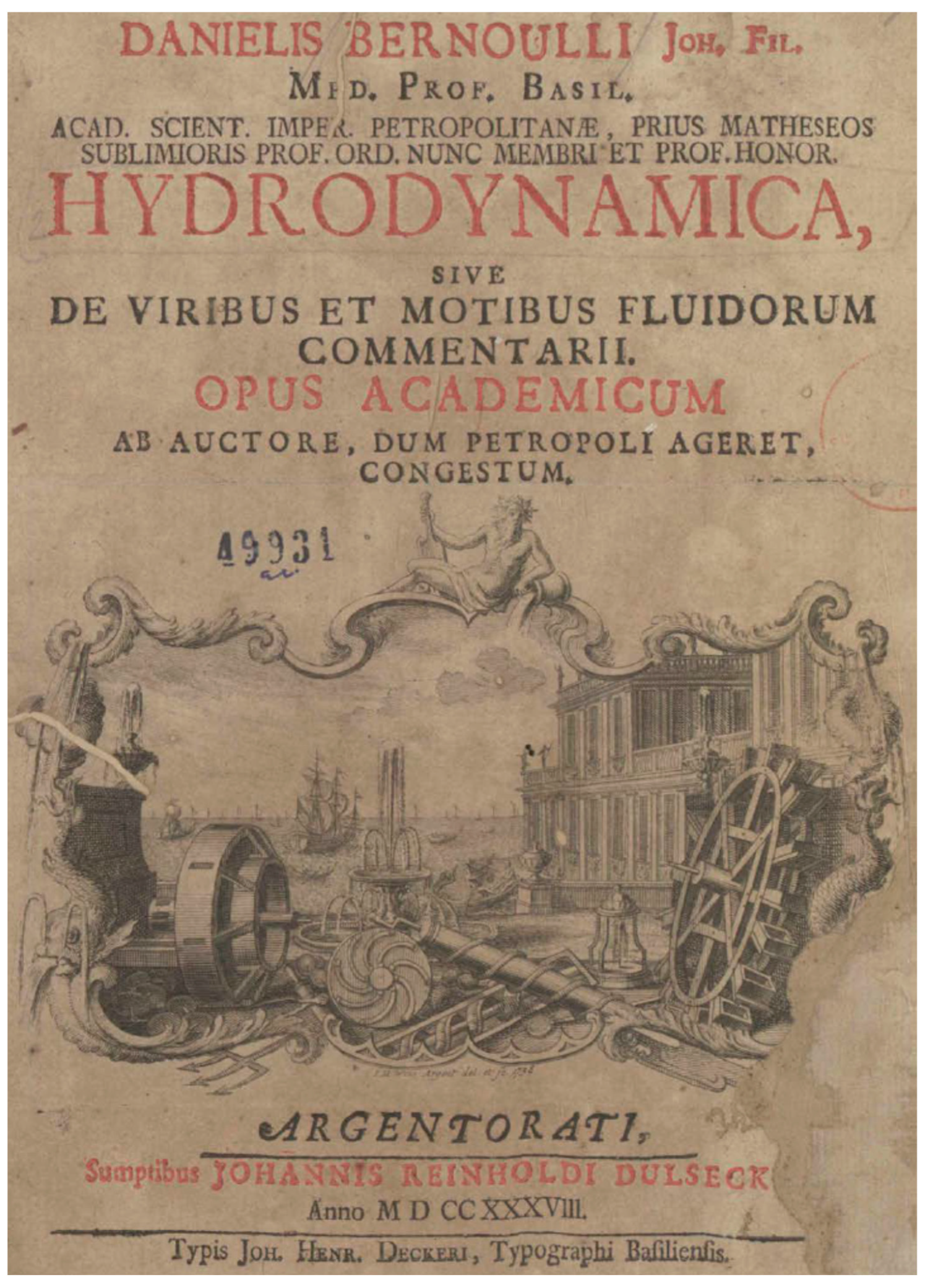
In the 16th and 17th centuries, a drastic change in scientific thinking took place, paving the way for the Scientific Revolution. Some of the key changes during this period included an emphasis on empirical observation and experimentation, leading to the rejection of the prevailing Aristotelian worldview. Additionally, there was a shift towards using mathematics as a tool to describe and understand natural phenomena, the development of the scientific method, the invention of the printing press enabling the dissemination of scientific ideas, and the exploration and expansion of empirical knowledge. The era also witnessed the development of new tools and instruments and posed challenges to established religious and political authorities due to scientific discoveries and new ideas. This transformative period culminated in 1687 with the publication of Newton’s Philosophiæ Naturalis Principia Mathematica [4]. As a reflection of this change, known as the Scientific Revolution, the Royal Society of London for Improving Natural Knowledge was created in 1662, and the Académie des Sciences de Paris was established in 1666 [5]. The development of physics required better mathematical tools. At the end of the 16th century, the French mathematician François Viète (1540–1603) wrote the first work on symbolic algebra, introducing the use of letters to represent quantities [6]. Another significant contribution was made by René Descartes (1596–1650), who reduced geometry to equations [7]. This process peaked with Newton and Leibniz, who established modern calculus. It is important to keep in mind that, at that time, the concepts of momentum and energy were not yet well established. Regarding the driving force that puts bodies in motion, in the 18th century, the focus (and result of its application) varied, depending on the school or doctrine to which the researcher adhered. Thus, the Cartesians indicated that it was momentum, the Newtonians the variation of momentum, and the Leibnizians the conversion of vis morta to vis viva (a concept that we now associate with energy). It was Pierre Varignon (1654–1722) who, applying the calculus developed by Leibniz to the mechanics presented by Newton, analytically determined the exit velocity through an orifice based on the concept of momentum, with an expected error coefficient of [8]. In 1738, Daniel Bernoulli (1700–1782) published Hydrodynamica, sive de viribus et motibus fluidorum commentarii [9] (Figure 2), in which he used what we call nowadays the energy approach for the first time to address the problem and correctly obtain Torricelli’s expression for discharge through an orifice. The English translations of Daniel Bernoulli’s Hydrodynamica and Johann Bernoulli’s Hydraulica were published in 1969 in a single book by Dover Publications Inc. Following Leibniz, whose formulation of energy concepts was based on the fall of particles, the energy conservation applied by Bernoulli considers only the terms associated with what we now call kinetic energy (vis viva, “living forces”) and potential energy (vis morta, associated with pressure or weight).
Jean Le Rond D’Alembert (1717–1783) demonstrated the conservation of “living forces” and in 1744 published Traité de l’équilibre et du mouvement des fluides, in which he formally proved the results of Bernoulli. In this work, he considered that the equilibrium that exists between the “parts” of fluids, despite the difference in pressures, is due to the adhesion between particles, and in Chapter IV he asks: “Is this force purely passive, that is, only due to the roughness of the fluid particles that touch each other, or is it an active force that tends to unite these particles and bring them closer together?” [10] (p. 37). In 1768, in the first part of volume 5 of Opuscules Mathématiques, D’Alembert published the article Paradoxe proposé aux Géometres sur la Resistance des Fluides, in which he demonstrated that the force due to the motion of an incompressible fluid over an axisymmetric obstacle, whose geometry of the half facing the flow is equal to the rear, is zero. Unable to explain the reason for this result, he concluded the article by writing that it is a “singular paradox that I leave for geometers to clarify” [11].
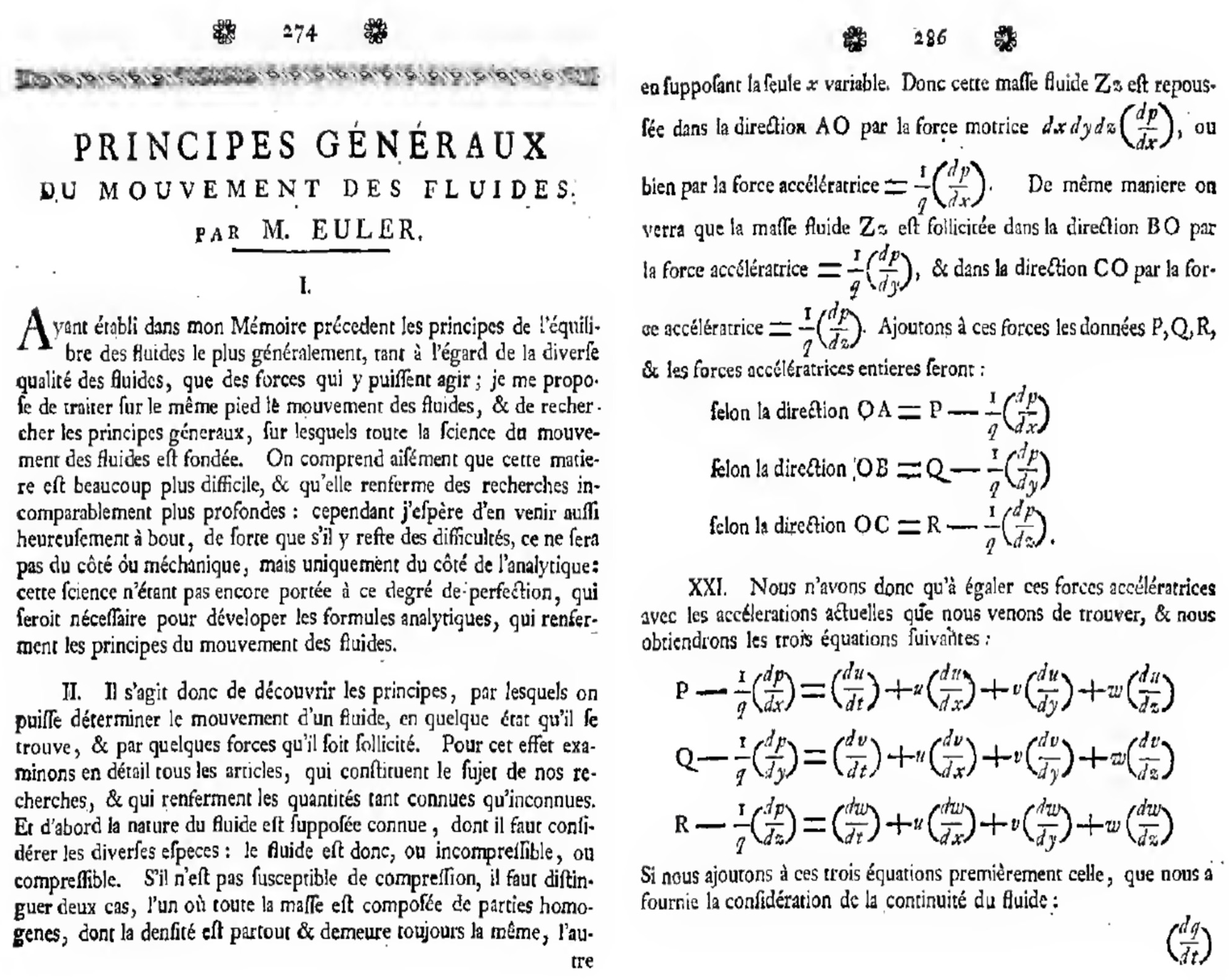
Significant advances to Newtonian dynamics were made by Leonard Euler (1707–1783). Newton’s work basically referred to particle dynamics in one dimension. In 1750, Euler presented the equations for the generalised motion in the three spatial dimensions, which were published in 1752 in an article titled Découverte d’un nouveau principe de mécanique [12], in which he extended the second law of Newton to a continuous medium. In 1757, the works presented in 1755 were published in the Mémoires de l’Académie Royale des Sciences et Belles-Lettres de Berlin. The Mathematics section presents three works by Euler: Principes généraux de l’état de l’équilibre des fluids [13], Principes généraux du mouvement des fluids [14], and Continuation des Recherches sur la théorie du mouvement des fluids [15]. In the second of these, Euler derives the components in the three spatial directions of the equation of motion of the ideal fluid, currently known as the Euler equation (Figure 3). Joseph-Louis Lagrange (1736–1813), among his many contributions to mathematics and physics, in his Mémoire sur la théorie du mouvement des fluids [16], uses the potential function to describe the motion of fluids.
3. Structure of the Matter: Continuum or Atomic?
D’Alembert, Euler, and Lagrange made extensive use of differential equations, using the calculus tools developed up to that time. This meant that they considered matter as a continuous medium. However, this assumption generated some problems, for example, when trying to explain the deformation of solids or the vortices and eddies in what we now know as turbulent flows. This development of hydrodynamics, called “analytical mechanics”, contrasts with what would later be called “physical mechanics”, which was based on the interaction of molecules [17] (p. 361). This division continued to be present in the teaching of mechanics at the École Polytechnique at the end of the 19th century, as shown by Boussinesq in his Leçons Synthétiques de Mécanique Générale servant d’Introduction au Cours de Mécanique Physique (Synthetic Lessons of General Mechanics serving as an Introduction to the Course of Physical Mechanics), printed in 1889 [18]. Boussinesq was a defender of physical mechanics and indicated that rational (or analytical) mechanics was insufficient for the study of the most important phenomena and that the “material points” that arise from the atomic hypothesis for the constitution of matter allow us to explain the behaviour of matter by considering the interaction between them, as indicated in the first lesson of his Leçons Synthétiques [18].
The idea that matter was composed of atoms was not new. Already in the 5th century BC, the presocratic philosophers Leucippus of Miletus and his disciple Democritus of Abdera had proposed it. The ideas of Leucippus and Democritus were reformulated in the philosophy of Epicurus (c.341–c.270 BC), and the atomistic physics derived from it was presented by the Roman poet and philosopher Lucretius (98–55 BC) in his verse work De Rerum Natura (On the Nature of Things). Rodríguez-Navas, in his Spanish translation, in prose, published in 1892, says, “Deliberately, no doubt, Lucretius did not use the word ‘atom’ even once in his entire extensive poem, which encompasses the subject most thoroughly studied in all his work” [19] (p. 4). The conception that matter is made up of atoms or fundamental particles was transmitted through the centuries and commented on, modified, or questioned by different authors, including Galileo Galilei (1564–1642), Thomas Hobbes (1588–1679), Robert Boyle (1627–1691), Robert Hooke (1635–1703), Christiaan Huygens (1629–1695), and Isaac Newton (1642–1727). Of the aforementioned, Boyle, Hooke, and Newton considered that heat was associated with the vibration of atoms or basic particles. Atomism was not free from detractors, especially for religious reasons, such as those made by St. Dionysius of Alexandria (3rd century) and with great force in the period 1660–1700, when it began to be considered with a more scientific than philosophical approach. The Parliament of Paris decreed in 1624 that those who supported or taught atomism would be subject to the death penalty [20]. Chapter 4 of Whyte’s book (reference [20]) contains a chronological table, which has been the basis for what is presented here regarding the development of atomistic ideas.
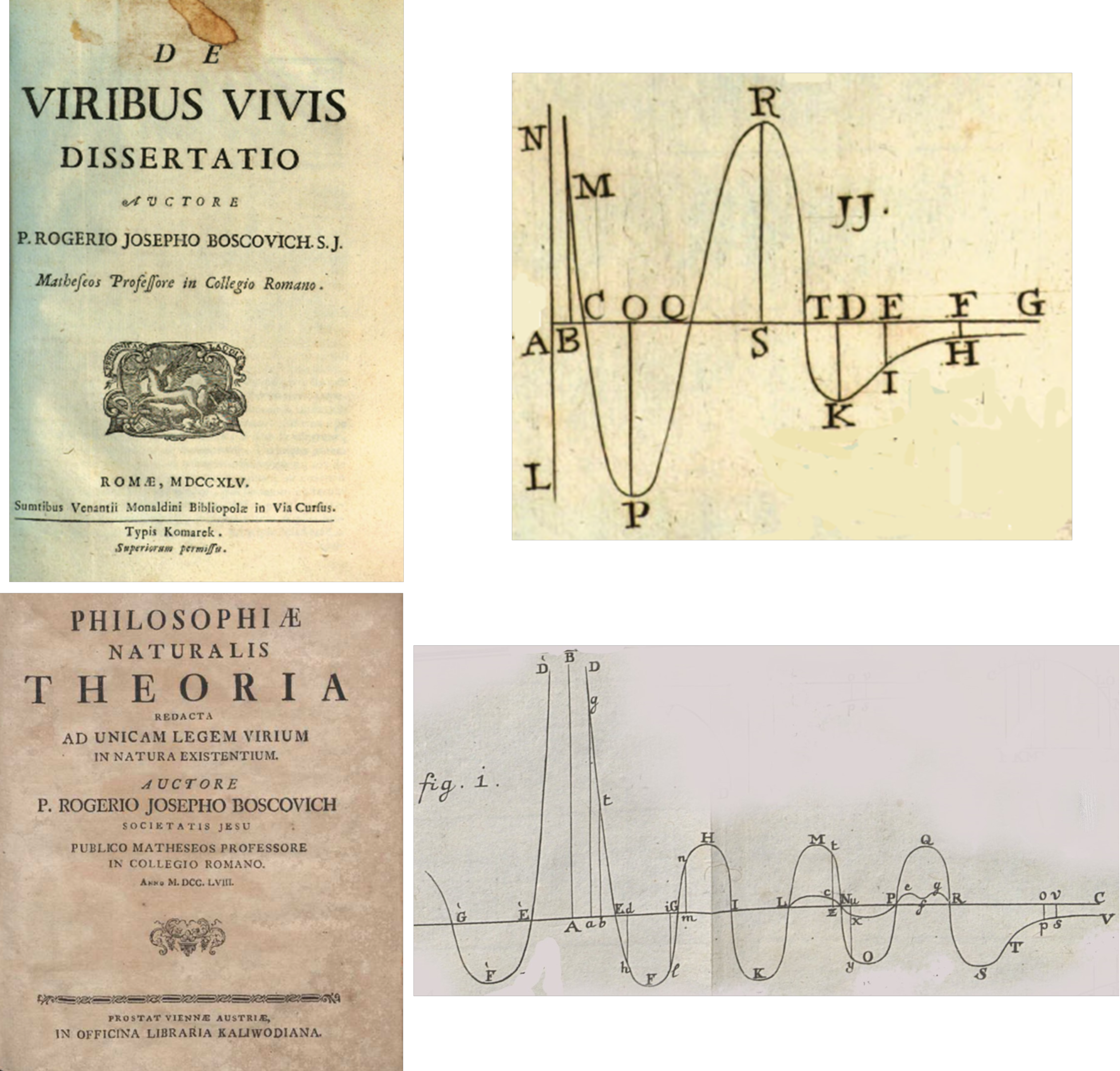
Concerning the forces between basic particles, Newton postulates in his Philosophiæ naturalis principia mathematica [4] that they can be either attractive or repulsive (the latter being distinct from gravitational), and he demonstrates Boyle’s law for gases by considering that the force of repulsion is inversely proportional to the distance between the centers of the particles (Proposition XXIII, Theorem XVIII of Book 2; [21]). Newton does not write but instead does so descriptively, without equations. Another important contribution regarding the forces of interaction between particles was made by the Croatian Rudjer Josip Bošković (1711–1787, also called Ruggero Giuseppe Boscovich), who published two important works related to the atomic (or molecular) structure of matter: In 1745, De Viribus Vivis Dissertatio, and in 1758, Theoria Philosophiæ Naturalis, with a revised and improved edition in 1763. In them, he postulates the existence of attractive and repulsive forces between atoms (or molecules), depending on the distance between them. If the atoms are far enough apart, the force is Newtonian attraction (proportional to the inverse square of the distance), but when they are very close, it is repulsive, asymptotically tending to an infinite value as the separation approaches zero. Between these two extreme behaviors, the force is finite and oscillates between attraction and repulsion. Figure 4 shows the graphical representation of these forces, taken from Boscovich’s publications of 1745 and 1758 [22,23].
Pierre Simon Laplace (1749–1827) considers the molecular structure of matter and presents it in his successive editions of Exposition du Système du Monde (1796 [24], 1799 [25], and 1808 [26]), in each of which he improves his arguments. In a publication from 1805, he explains capillary rise through a molecular approach [27] (p. 1) and indicates that these molecular attraction forces “are insensible to sensible distances”. This idea of molecular forces whose spatial action is very limited is refined in the third edition of his Exposition, in which he includes a chapter titled “On molecular attraction”, where he reinforces the idea that molecular forces are “sensible only to imperceptible distances”. The molecules are subject to an attraction force that decreases extremely rapidly [26] (p. 316) and to one that opposes it, due to heat, which also has the effect of decreasing their viscosity or intermolecular adhesion [26] (p. 317).
4. Navier’s Equation
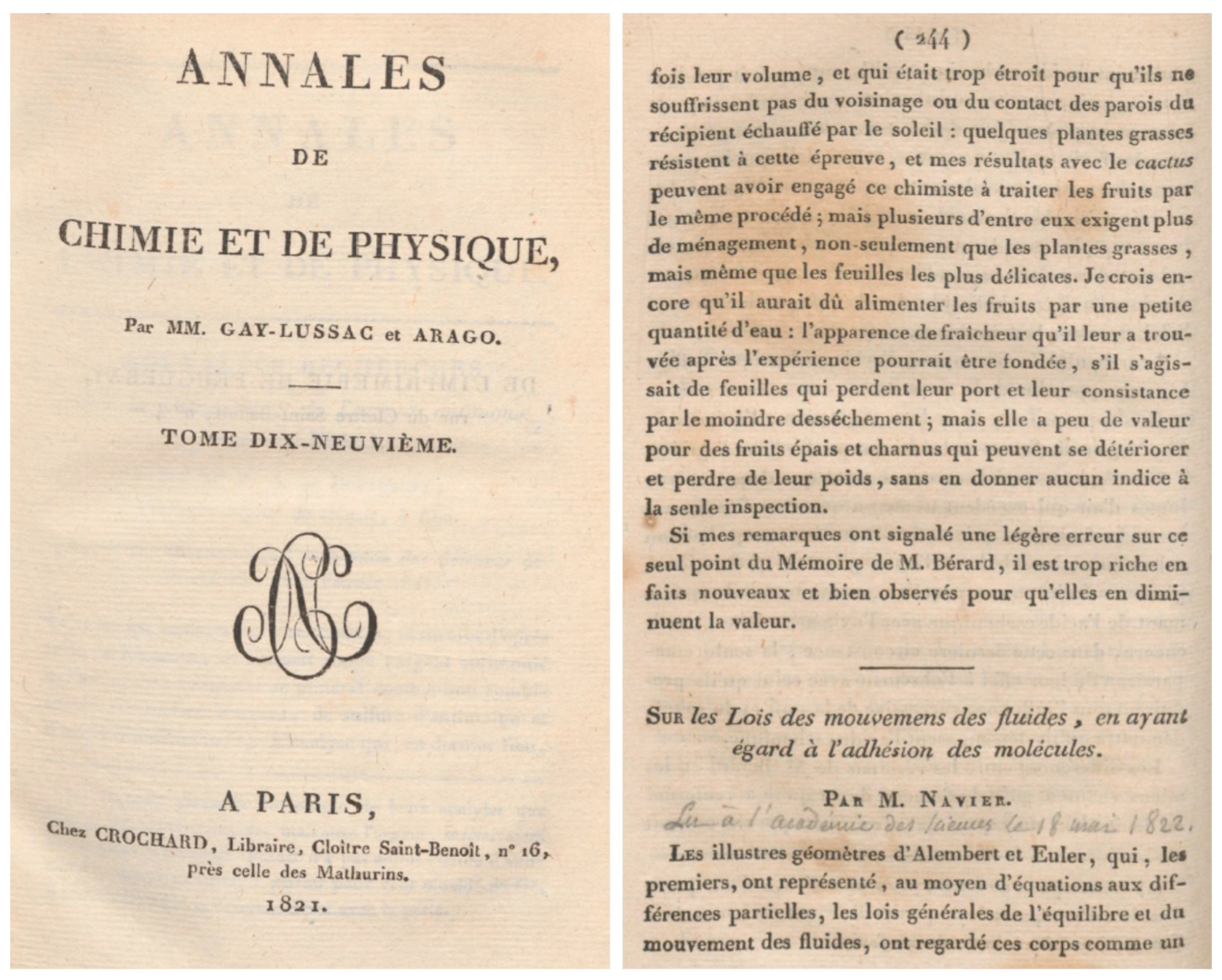
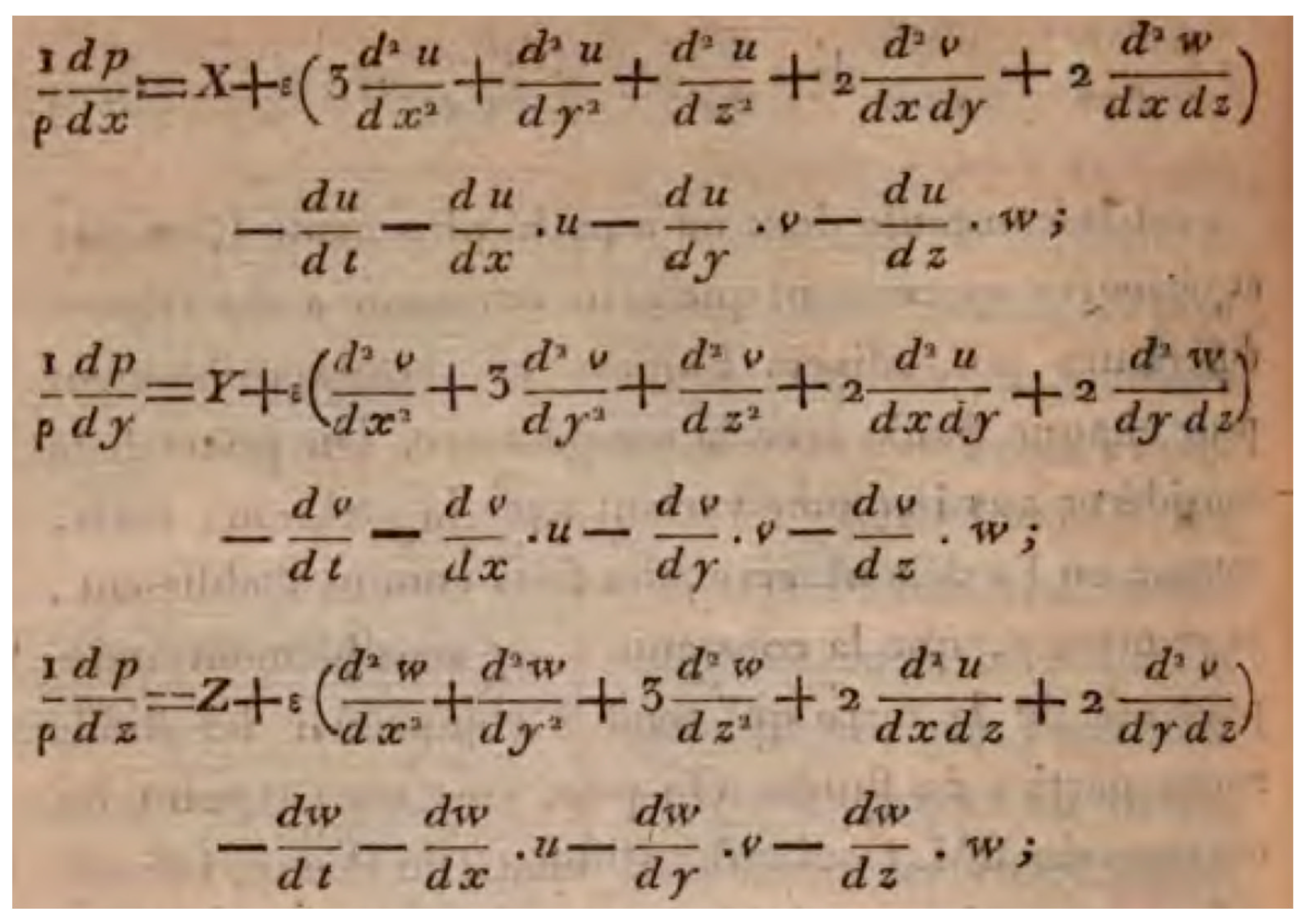
With the concepts of intermolecular forces presented above, Navier approached the study of fluid motion. Navier deduced and presented his equation for incompressible fluids in two articles. The first, published in 1821 in the Annales de Chimie et de Physique (Figure 5), titled Sur les Lois des mouvemens des fluides, en ayant egard à l’adhesion des molecules [28], does not detail the algebraic deduction of the term associated with flow resistance. The momentum equations that Navier arrived at are presented in Figure 6, where , and correspond to the components of the body force, which, a few lines later, he considers to be gravitational. Note that in the notation of the time, there was no differentiation between the partial derivative , … and the total derivative , …. It is interesting to see that the terms associated with molecular resistance (those that accompany the coefficient) are not presented in reduced form, resulting when using the continuity equation. For example, with modern notation, the term in parentheses for the component along can be written as:
reducing to when the continuity equation is imposed for an incompressible fluid:
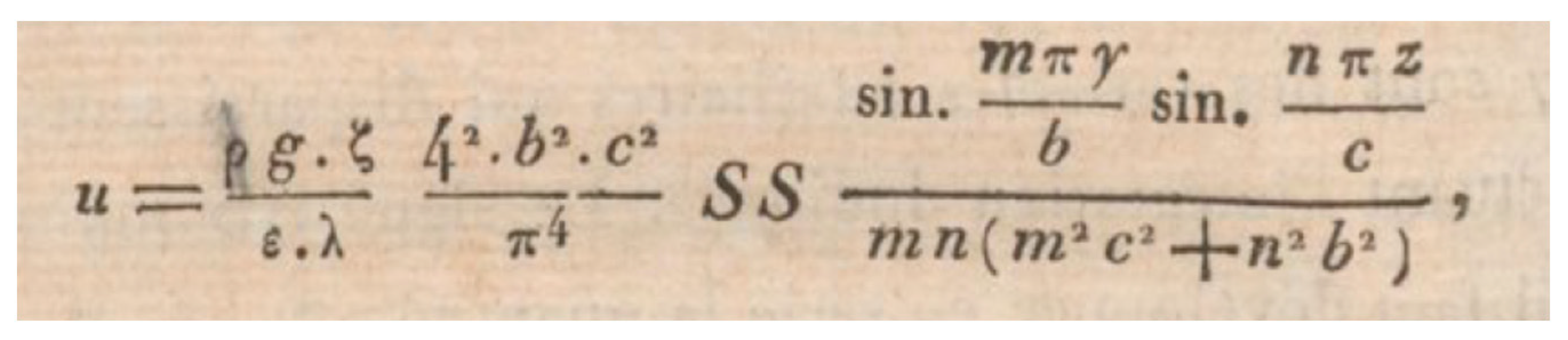
Navier’s first application of his equations corresponds to the flow generated by a pressure gradient in a very long (in the -direction), rectangular cross-section pipe that is inclined, such that “all the fluid molecules move parallel to each other”. The fluid is initially at rest, so the solution depends on . The boundary condition corresponds to zero velocity at the wall, which Navier justifies with the argument “…there exists an extremely thin layer of motionless fluid against solid walls, or these walls are formed by the very substance of the fluid, which would have solidified”. For any given time, the resulting velocity distribution occupies a couple of lines of the page, and for , it reduces to the expression presented in Figure 7. In that equation, represents the hydraulic head and represents the length of the pipe. is the coefficient of molecular attraction, which Navier rigorously deduced and presented in his article published in 1823 [29].
In order to compare his theoretical result with experimental data, Navier determined the average velocity for a rectangular pipe with sides and using the theoretical expression for velocity distribution obtained from the equations of motion (Figure 7). He compared his result with the data taken by Girard, presented in l’Académie de France in 1816 and published in 1818 [30].
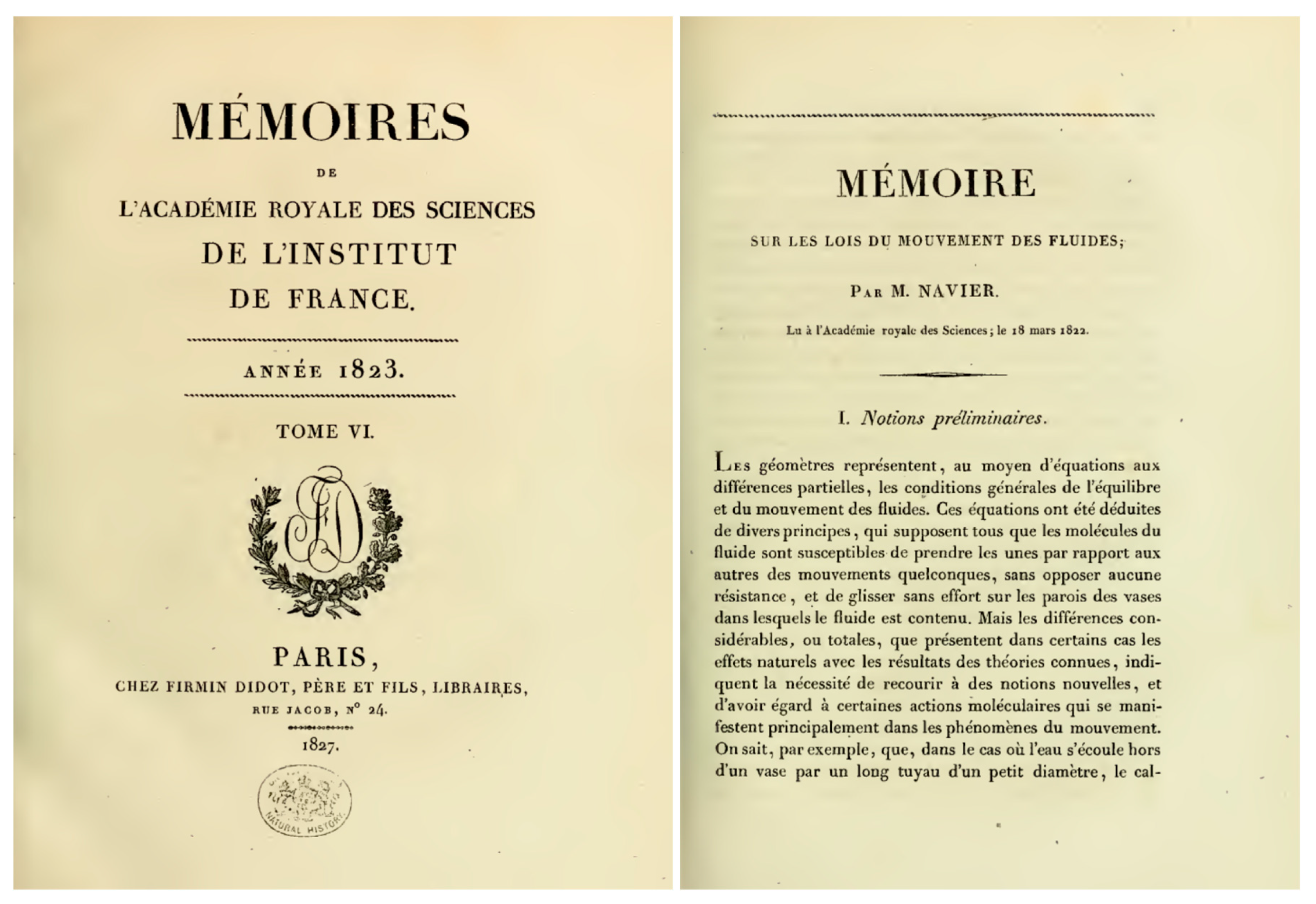
On 18 March 1822, Navier presented his Mémoire sur les Lois du Mouvenment des Fluides at the Académie Royale des Sciences in Paris, which was published in the Volume VI, corresponding to 1823, but issued in 1827, of the Mémoires de l’Académie des Sciences de l’Institut de France [29] (Figure 8). In this work, Navier considers the fluid as incompressible and consisting of “a set of material points, or molecules, located at very small distances from each other, and capable of changing almost freely their relative positions”. The pressure exerted on the fluid “and penetrating into the interior of the body”, “tends to bring the parts closer, which resist this action by repulsive forces that are established between neighbouring molecules”. In the hydrostatic condition, “each molecule is in equilibrium, subject to these repulsive forces and external forces, such as gravity, which may act on it”. Furthermore, “the actions exerted from molecule to molecule within bodies vary with the distance between the molecules”, so that if the distance between them is reduced, a repulsive force is generated, and if it is increased, an attractive force is created. When the fluid is in motion, Navier considers that “two molecules that approach each other repel with greater force, and two molecules that move away from each other repel with less force”, so that “the repulsive actions of the molecules increase or decrease in an amount proportional to the velocity with which the molecules approach or separate from each other”. These same forces also act between the molecules of the fluid and those of the walls of the solid that contains them.
For the hydrostatic equilibrium condition, Navier analyses the interaction between two neighbouring molecules, M and M’ (Figure 9), with coordinates and , so that the distance between them is . It is necessary to note that in the article, is used interchangeably to indicate the distance between the two molecules M and M’ as well as to designate the density of the fluid. By designating as the force between the two molecules and as the moment of between the two molecules, the moment on molecule M resulting from the action of the 8 molecules surrounding it in an arrangement as indicated in Figure 9, turns out to be (using the current notation for partial derivatives):
In the static condition, where there is a balance between the pressure force and the repulsive forces, the following holds true:
Then, Navier relates the pressure to body forces for the hydrostatic condition, which in modern notation is written as , where is the body force vector (per unit mass) and in this case denotes the fluid density.
Once the static problem is solved, Navier addresses the case where the fluid is in motion, which induces other forces of molecular interaction, and “the main objective of the work is to find analytical expressions for these forces”. To do this, he considers that there is a relative motion between the molecules M and M’, whose velocities are, respectively, and
obtaining that the moment of the forces resulting from the mutual action of M and M’ is given by
From the interaction between two molecules, given by the previous expression, Navier obtains the result for the eight molecules surrounding it, which is presented in Figure 10.
As mentioned, the expression in Figure 10 corresponds to the effect that the surrounding molecules have on one molecule. To consider all the molecules in the fluid, it is necessary to integrate over the entire flow domain, which can be considered infinite in terms of the dimensions associated with the molecules. This integration is facilitated by working in spherical coordinates, resulting in:
In the determination of the value of , Navier indicates that the sum of moments was considered twice, so the numerical coefficient of Equation 6 must be divided by 2. Navier repeats the analysis for the case of molecules that are in contact with the solid wall (which he denotes m), with an interaction force , resulting in:
is a constant that must be determined experimentally and depends on the nature of the wall and the fluid, and it can be considered “as a measure of their reciprocal action”. After analysing the dynamic equilibrium and a lot of algebra, Navier obtained the set of differential equations that, according to him, govern the motion of incompressible fluids (Figure 11, where , and are the components of the body force per unit volume, i.e., , and considering the gravity force field, in current notation, is written as:
Note that in the previous equations, the coefficient is unknown since it depends on the intermolecular force , of which it is only known that it decreases very rapidly with distance, so its range of action is very small (“they are insensible to sensible distances”, as Laplace wrote). It is also known that “this constant has different values for different fluids and varies significantly for each fluid with temperature” and that it is “sensibly independent” of pressure [28] (p. 251).
Regarding the boundary conditions, Navier indicates that fluid molecules in contact with the wall cannot move in the normal direction to it, so for a wall in the plane, it must satisfy:
Similarly, for walls in the and planes:
In the case of a free surface, . The boundary conditions given by Equations (11)–(13) are now called “Navier’s conditions”, allow for slip velocity at the wall, and are applied, for example, in modelling the flow of superhydrophobic fluids.
Navier concludes his work by applying the obtained equations to three cases: (i) Flow in a straight rectangular pipe, (ii) flow in a straight circular pipe, and (iii) flow with a free surface in a rectangular channel. For all three cases, the boundary conditions he uses are those given in the preceding equations. The problems in pipes are transient; the flow starts from rest and asymptotically reaches the steady state. The flow of case (i) is the same as that solved in his 1821 publication [28], but at that time, the boundary conditions applied were not Navier’s conditions but non-slip conditions at the walls.
5. Viscosity
Before continuing, it is worth reviewing the history of the word and concept of fluid viscosity. It is common in introductory fluid mechanics courses to present the property “viscosity” based on a flow with parallel streamlines (Figure 12) and postulating the proportionality between the shear stress () applied to an element of fluid and its rate of angular deformation (, which is demonstrated to be equal to the velocity gradient ). The proportionality coefficient corresponds to dynamic viscosity. This is how it is shown, for example, in the texts by White [31] (pp. 22–23), Massey [32] (pp. 21–24), and Munson et al. [33] (pp. 14–15), where it is stated that . Directly in the form as Newton proposed it, that is , it is presented, among others, in the texts by Granger [34] (pp. 41–43), Streeter et al. [35] (pp. 8–9), and Shames [36] (pp. 10–12).
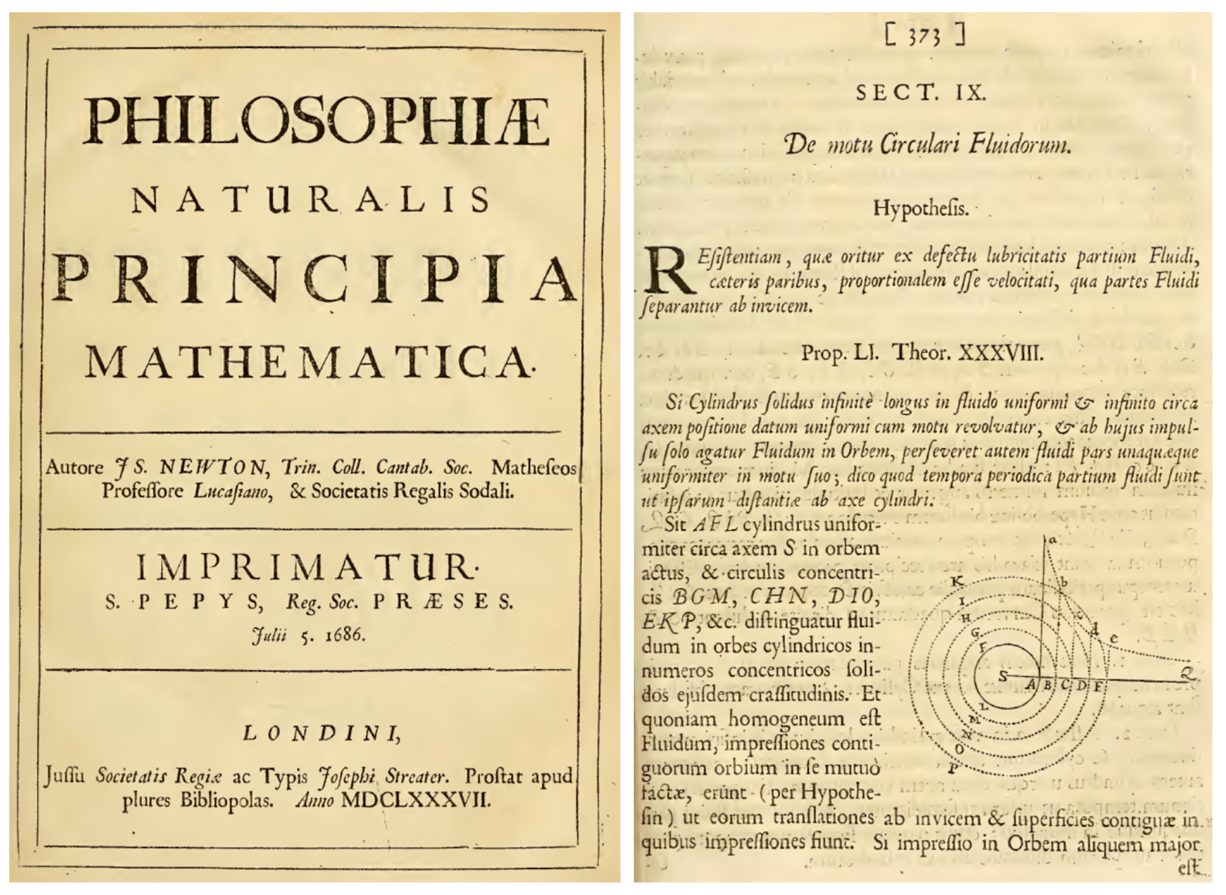
Newton, in the first edition of 1687 of his Principia [4], as in later editions, did not propose the parallel straight-line motion shown in Figure 12, but instead established the proportionality between shear stress and velocity gradient in the part of his Principia concerning the circular motion of fluids. In Book II, Section IX (Figure 13), he postulated that “the resistance arising from the lack of lubricity in the parts of a fluid is, other things being equal, proportional to the velocity with which the parts of the fluid separate from each other” [21].
Note that Newton does not mention the word “viscosity” or “viscous”, but instead refers to the “lubricity” of fluid particles. According to the Online Etymology Dictionary, www.etymonline.com (accessed on 1 September 2023), the word “viscosity” was first recorded in English in the early 15th century and comes from the Old French “viscosité”, which was recorded in the 13th century, or directly from Medieval Latin (6th–14th centuries) “viscositatem/viscositas”, a word that, in turn, comes from Late Latin (3rd–6th centuries) “viscosum”, which means “sticky”. This last word comes from Latin “viscum”, which refers to mistletoe, a semi-parasitic plant that grows on the branches of certain trees and whose fruit is a berry containing a sticky (or viscous) pulp. In Spanish (https://iedra.es/, accessed on 1 September 2003), the first recorded use of the word “viscoso” (sticky) in a dictionary is in 1570, in Cristóbal de las Casas’ “Vocabulario de las dos lenguas Toscana y Castellana” [37], and the word “viscosidad” is first recorded in 1617 in John Minsheu’s “Vocabularium Hispanicum Latinum et Anglicum copiossisimum”. The Royal Spanish Academy (Real Academia Española), founded in 1713, records both words in its first edition of “Tomo Sexto del Diccionario de la Lengua Castellana”, printed in 1739 [38] (p. 437 and 438), with the meaning of “sticky matter or humour” for viscosity and “sticky or glutinous” for viscous.
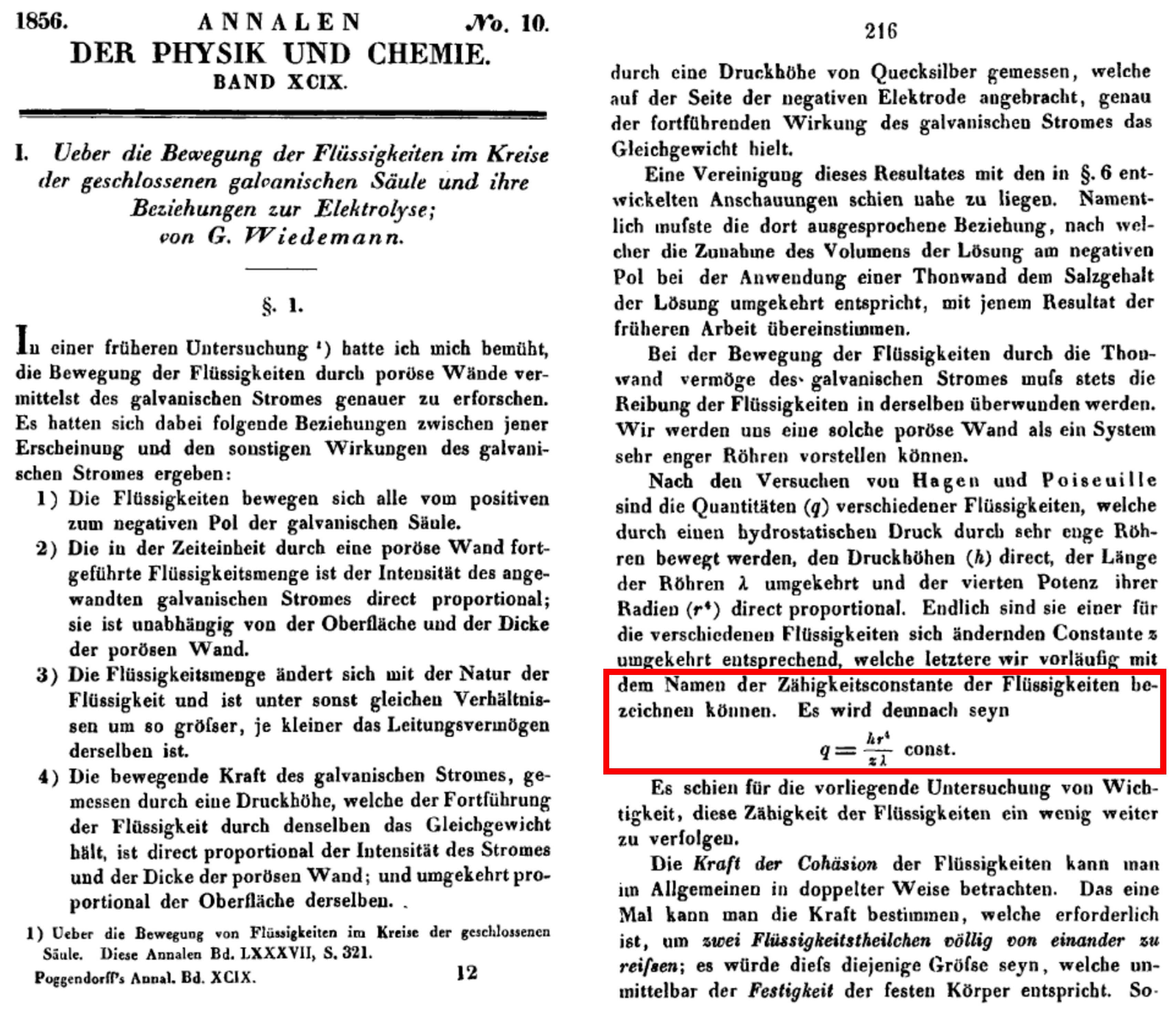
The first use of the term viscosity with a physical meaning was by Wiedemann in 1856, in a study related to the flow induced by electrolysis in saline solutions, using the expression Zähigkeitconstante der Flüssigkeiten, “viscosity constant of liquids” [39] (Figure 14). Note that neither Cauchy [40], nor Poisson [41], nor Saint-Venant [42], nor Stokes [43] used the word “viscosity” in their publications on the equations of fluid motion. Stokes, in his work, expresses “The amount of internal friction of water depends on the value of ”, without explicitly defining what the coefficient is. More than 20 years later, the use of the term viscosity could even harm the publication of an article. This is reflected in one of the letters from the extensive correspondence between Saint-Venant and Boussinesq. In a letter dated 12 July 1868, the septuagenarian Saint-Venant advises the young Boussinesq, regarding a manuscript that the latter wanted to publish, to avoid using “viscosity” in the title and other places in the work, as that would give the reviewer arguments to make comments and thus make it difficult to accept the article, suggesting that he “change the title, for example, to: The influence of internal and external friction (or tangential actions) on the motion of fluids”. Promptly, on 14 July, Boussinesq replied, “I think I must tell you at once that there is no opposition to you in my manuscript dealing with the friction of fluids…I use the term friction everywhere instead of the term viscosity” [44]. Note that as late as 1886, it seemed appropriate to define viscosity, as did Reynolds in his article “On the Theory of Lubrication …” [45] (pp. 164–165), where he defined “the coefficient of viscosity, or, commonly, the viscosity of the fluid” as “the shearing stress divided by the rate of distortion”.
6. The Other Equations of Fluid Motion
The equation presented by Navier in 1822 was rederived at least four more times: By Cauchy in 1823, Poisson in 1829, Saint-Venant in 1837, and Stokes in 1845. Each of the authors of the new derivations ignored or criticised the development of their predecessors, justifying the conceptual foundations of their own deduction [2]. It is interesting to note the close relationship between the development of equations governing fluid motion and those for elastic solids. Developed for one material, the concepts were applied to the other, which in practice means replacing displacements of molecules (solids) with displacements per unit time (fluids). Darrigol’s work [2] presents this parallel development in a lively manner (using current vector and index notation). Without going into further detail regarding the deductions made by the different authors, the equations governing fluid motion obtained by them are presented below. The following subsections take the article by Darrigol as their main reference.
6.1. Augustin-Louis Cauchy (1789–1857)
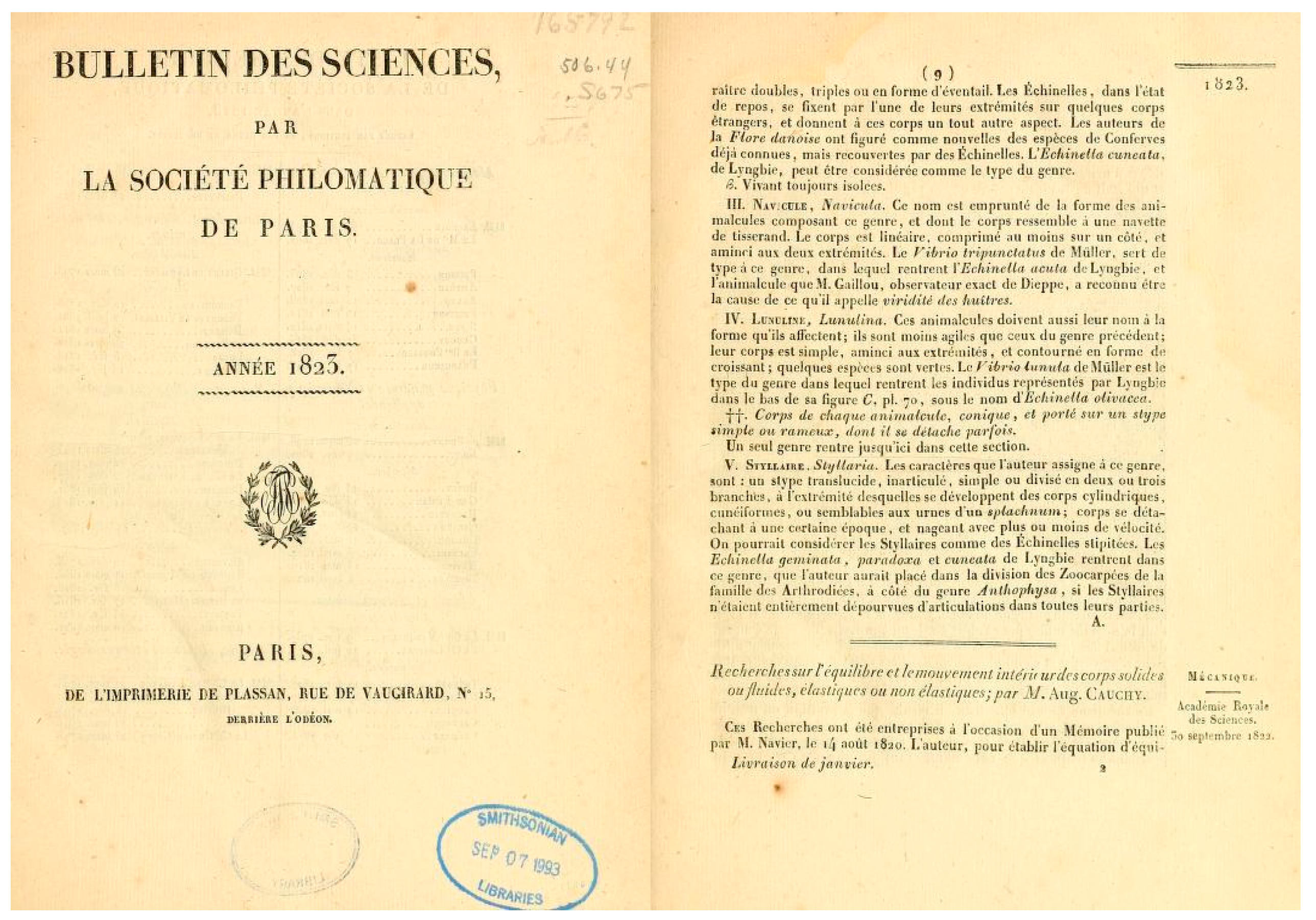
On 30 September 1822, Cauchy presented the results of his study at the Académie Royale des Sciences in Paris, and a summary was published in 1823 in the Bulletin des Sciences by the Société Philomathique de Paris [40] (Figure 15). In his work, Cauchy analysed Navier’s work regarding the restoring forces of a solid subject to dilation and flexion. According to Navier, two types of restoring forces are required, but Cauchy concluded that the second was not necessary if it was considered that the first was not perpendicular to the section on which it acted. In other words, the pressure does not act normal to the surface; that is, there are normal and tangential stresses whose resultant is a stress (“pressure”) not perpendicular to the surface. Although other authors such as Coulomb, Young, and Navier had considered the presence of what we now call shear stresses in certain beam-breaking problems, Cauchy was the first to propose an elasticity theory based on a general definition of internal stresses. Cauchy demonstrated three fundamental theorems of elasticity, which in current language are: (i) the stress tensor is a second-rank tensor ( 3 × 3 matrix), (ii) the stress tensor is symmetrical (), and (iii) the resultant of the forces acting on a volume element, per unit volume, is given by .
To apply the ideas developed for solid bodies to fluids, Cauchy considered an infinitesimal element of “solidified fluid”, on whose surfaces normal and tangential stresses, , act. In his work, Cauchy proposed a constitutive law with two constants, which we now call viscosity and second coefficient of viscosity.
6.2. Siméon-Denis Poisson (1781–1840)
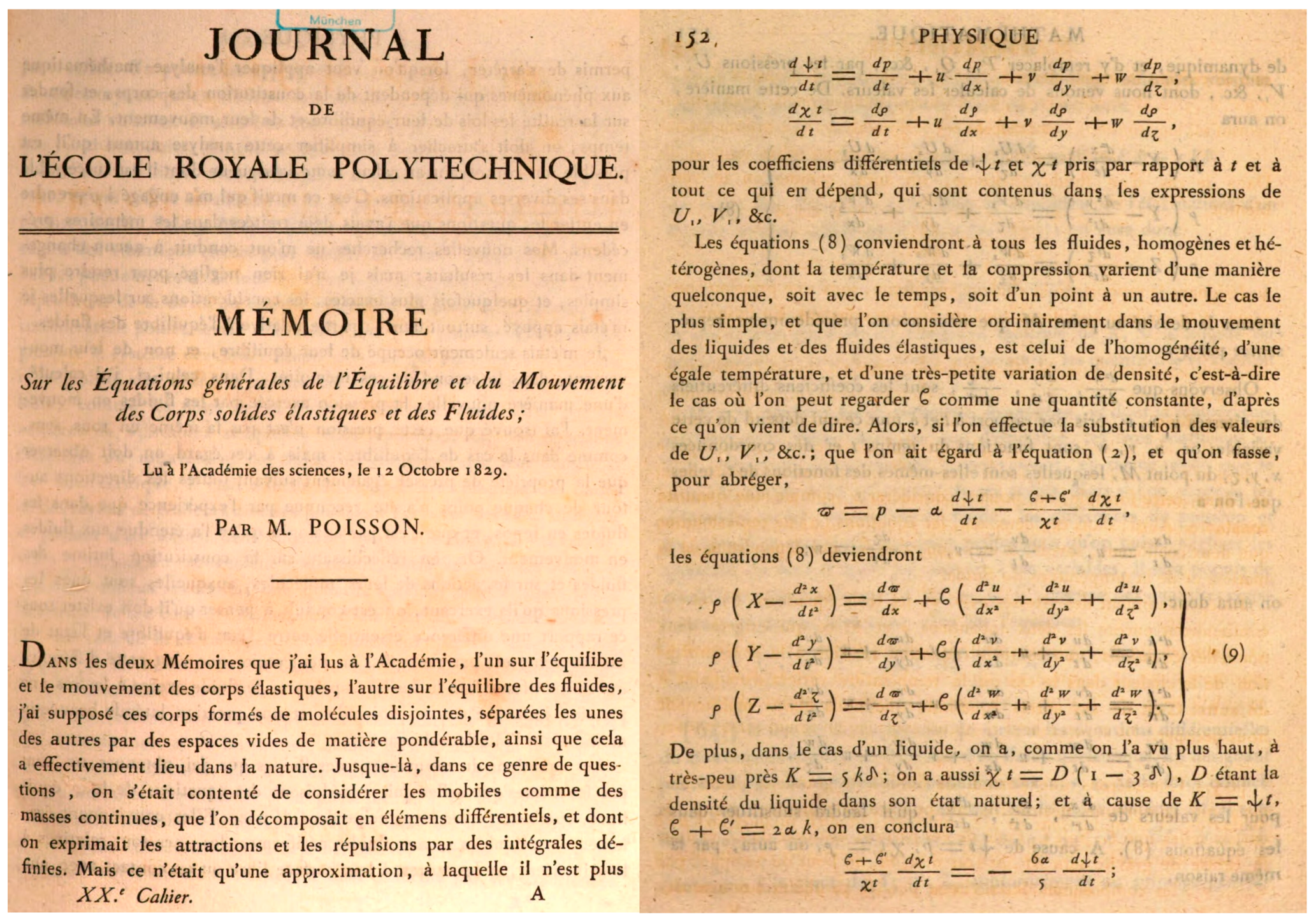
Like Navier and Cauchy, Poisson studied both the behaviour of elastic solids and the movement of fluids. In his article read in 1828 and published in 1829 [17], Poisson followed Navier’s line to obtain the equations of elasticity, considering molecular attraction forces, with some differences. For example, he did not use the method of moments but directly summed the molecular forces acting on a particular molecule. In another paper, read on 12 October 1829, at the Académie des Sciences de Paris and published in 1831 in the Journal de l’École Polytechnique [41] (Figure 16), he considered that a fluid element is subject to shear stresses during its movement, which spontaneously relax very rapidly, alternating the fluid in rapid states of stress and relaxation. He supposed that the stresses on the fluid element are proportional to the rate of deformation, analogous to his assumption that the stresses acting on an isotropic elastic solid body element are proportional to the deformation.
6.3. Adhémar Jean Claude Barré de Saint-Venant (1797–1886)
Saint-Venant is known in the field of hydraulics for his deduction of the equations that bear his name that describe gradually varied transient flow in open channels (published in 1871 [46]), but his contributions in other aspects of fluid mechanics, including his visionary conception of turbulence and particularly the idea of turbulent viscosity (which he transmitted to Boussinesq, who found expressions for them), often go unnoticed or simply ignored. With a strong mathematical background, he sought to reconcile engineering applications and scientific support with the state of knowledge at the time regarding the physics of solids and fluids, based on the concept of molecular structure of matter. There is little doubt that he developed vector calculus in 1832, but it was only published in 1851 in class notes (Principes de mécanique fondés sur la cinématique) used in courses taught at the Institut Agronomique. Usually, Grassmann receives credit as the inventor of vector calculus due to the work published in 1844 [47]. At his death, at the age of 89, Saint-Venant had published around 160 articles, and several more were published posthumously. His main interest, as well as his greatest contributions, was in the area of elasticity.
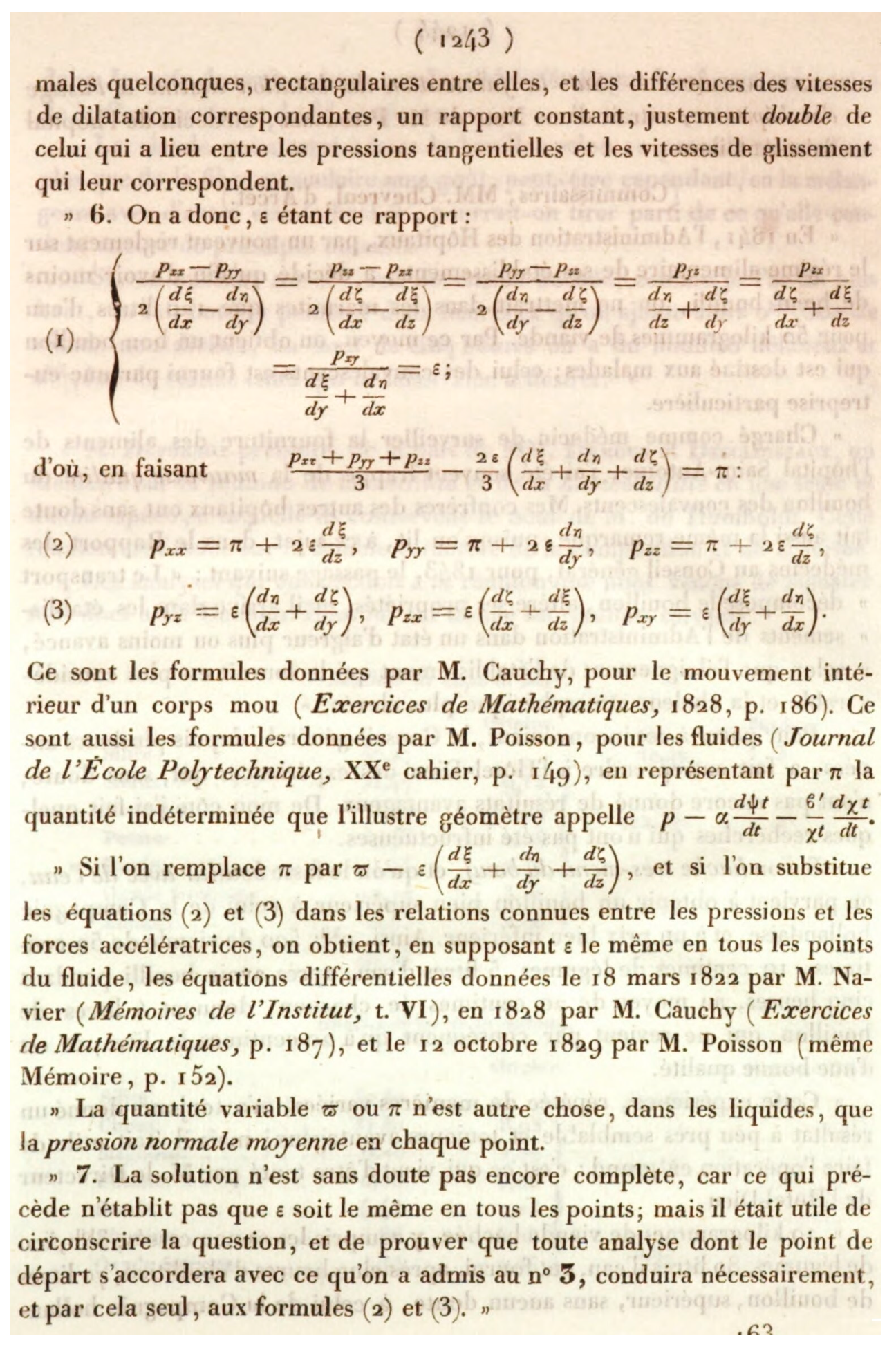
In the edition of 19 April 1834, of L’Institut, Journal Général des Sociétés et Travaux Scientifiques de la France et de l’Étranger, two abstracts of Saint-Venant’s work read in the session of April 14 are presented [48]. The first, in a short paragraph, refers to a general mechanics problem related to kinetic energy and work. The second abstract occupies almost an entire column of the magazine and is a review of studies on fluid dynamics, which mentions, among other topics, the demonstration of the existence of parallel pressures (resulting from friction) and normal to the direction of fluid movement. According to Darrigol [2], the complete work was never published. In 1843, Saint-Venant published a note to the 1834 work, in which he gives some details of the ideas developed almost a decade earlier [42]. In the note, he establishes that there is a proportionality between the differences in normal and tangential pressures, corresponding to the Navier’s or Poisson’s ϐ coefficient, as seen in Figure 17. Consistent with his denomination of “pressure” to what is currently called “stress”, he uses the letter instead of . Note that the notation used by Saint-Venant is the same used now to indicate the direction of stress and the normal to the surface on which it acts, i.e., . The note ends with the paragraph identified with 7 (Figure 17), where he states that “The solution is undoubtedly not yet complete, because the above does not establish that is the same at all points”. This comment, which may seem erroneous to us if we consider that is associated with viscosity, is not so when we pay attention to some paragraphs of other articles by Saint-Venant. For example, in his summary of L’Institut, he says: “the molecules, when passing each other, necessarily follow undulating trajectories, and the oscillations of their individual movements around the mean movement explain the internal friction of the fluids, which is essential to take into account, as well as the inequality between the pressures in a direction parallel and in a direction normal to the movements” [48]. In a footnote to the 1843 publication in Compte Rendu des Séances de l’Académie des Sciences of the article from 1834, Saint-Venant considered it important to clarify that “partial irregularities in the movement of a fluid require taking faces of a certain extension to have averages that vary regularly” [42] (p. 1242), that is, values of velocities and stresses averaged over the surface of the face are considered in the faces of the volume element. These irregularities in the movement, which could not be deduced from the Navier’s equation, arise from the observation of experiments in pipes and channels of an undulating or oscillatory motion, which we now associate with turbulence. In another article, published in 1838 [49], three pages long but with a long title: “Memoir on the Calculation of the Effects of Steam Engines, which contains general equations of the steady or periodic flow of fluids, taking into account their expansions and their temperature changes and without assuming that they move in parallel sections or by independent filaments”, Saint-Venant refers to the work of ordinary friction and the work of extraordinary friction, the latter determined by the swirling of fluid (“tournoiement du fluide”), especially in places where the flow section increases abruptly. In this way, it is possible to glimpse that Saint-Venant’s ε coefficient includes what, in modern language, we call molecular viscosity and eddy viscosity. It would be Boussinesq who would develop this idea in depth (which he undoubtedly discussed with his mentor Saint-Venant) and present it in his “Essai sur la Théorie des Eaux Courantes” in 1877 [50]. On page 7 of that essay, he writes, “M. de Saint-Venant seems to have been the first to point out the influence of vortex agitation on the coefficient of internal friction”. Later on, on the same page, he indicates that “everything we know leads us to infer that it must increase the coefficient of this proportionality (ε) with the dimensions of the cross sections”. Saint-Venant reasserted this idea when he wrote in 1851 that “this can be explained to some extent by noting that fluid layers do not move parallel to each other with regularly graded velocities from one to another, and that disruptions, vortices, and other complicated or oblique movements, which must influence the magnitude of friction greatly, are formed and developed even more in larger sections” [51] (p. 49). In a note from 1846 regarding the “retarding forces” of liquid motion, Saint-Venant indicates that internal friction depends on both the relative velocities of fluid particles and the dimensions of the section and distance to the wall. He concludes by saying, “this is what we can suspect from known facts that are difficult to explain in any other way” [52].
Undoubtedly, Saint-Venant’s contributions to hydrodynamics were transcendent, although his surname does not accompany the names of the equation of motion or the modelling of turbulence. The comments reproduced in the previous paragraph must be understood in the context of the knowledge that existed about fluid motion until the first three-quarters of the 19th century. Deductions, compatible with the molecular approach, led to equations of motion that presented two problems (in addition to the impossibility of finding a general solution to the differential equations, due to the presence of non-linear terms): A theoretical and an empirical one. The theoretical problem corresponds to the boundary condition that must be imposed: Is there or is there not slip of the fluid molecules in contact with the wall? The empirical problem is due to the fact that the results obtained from the application of the equations of motion only agreed with measurements made in capillary tubes or very small-diameter tubes. In larger-size channels and pipes, the flow rate and resistance did not match the theoretical result. In addition, a pattern of motion was observed that was not rectilinear but with “undulating trajectories” and the presence of vortices that, according to Saint-Venant, generated extraordinary internal friction (in opposition to the ordinary friction that was present for rectilinear flow). It would be necessary to wait for Reynolds to establish the difference between what we currently call laminar flow and turbulent flow, as well as the equations that govern the latter. But Saint-Venant already understood that he had to consider average quantities and that the internal resistance coefficient, , depended on both fluid properties (due to molecular attraction forces) and the flow and geometry of the channel. In current language, we would say that , i.e., the coefficient of internal friction (as Saint-Venant would say) has a viscous component and a turbulent component (). It was Boussinesq who published expressions for in 1877, and undoubtedly, they had been discussed with Saint-Venant. In general form, according to Boussinesq, depends on the position in the flow section and is given by:
where is the density of the fluid, is the acceleration due to gravity, is the flow area, is the wetted perimeter, is the mean velocity value at the wall, and is a functional relationship that depends on and . is a coefficient that depends on the size of the wall roughness, is almost independent of and slowly varies with the hydraulic radius [50] (p. 51). The dimensions of are .
Thus, we can see that Saint-Venant’s contribution goes far beyond the deduction of the equation of motion of fluids. Combining his acute analytical and observational skills, physical principles, and theory, he was able to anticipate what turbulence modelling would become by conceiving that local resistance to motion depends on both molecular factors and the integral properties of the flow. The success of the master can be seen through the work of his protégé, J. Boussinesq, who successfully applied Navier’s ideas to turbulent flow, considering average variables and a variable viscosity.
6.4. George Gabriel Stokes (1819–1903)
As we have seen, the equation of motion for fluids appears to be an exclusive creation of French minds, a result of the solid mathematical training provided at the École Polytechnique, which sought to generate advanced knowledge in mathematical physics in the context of engineering applications [2]. The interest of English scientists of that time was in astronomy or mathematics, and only tangentially in hydrodynamics or elasticity. The contributions of people such as George Airy (1801–1892), George Green (1793–1841), or Phillip Kelland (1808–1879), especially in the field of wave theory, were only by-products of their main interests. In this environment, we find Stokes, whose training was in mathematics.
The first article that appears in Mathematical and Physical Papers by George Gabriel Stokes, Vol. 1, published in 1880, which compiles Stokes’ work taken from the original publications “with additional notes by the author”, is titled “On the steady motion of incompressible fluids”, was read on 25 April 1842, and originally published in Vol. VII of Transactions of the Cambridge Philosophical Society [53,54]. The article considers two-dimensional irrotational flow “where the stream-lines are a system of similar ellipses or hyperbolas having the same centre, or a system of equal parabolas having the same axis” [54] (p. 446). When discussing the case of hyperbolas, he considers the discharge through an orifice from one fluid-filled tank to another, indicating the experimental result that the fluid “has a tendency to keep within a channel of its own, instead of spreading out” [54] (p. 447). In this way, Stokes is the first to relate the equations governing irrotational flow (Euler’s equations) with surfaces of discontinuity. But perhaps even more interesting is when he writes, “I have not proved that the fluid must move in this system of lines … there may be perhaps different modes of permanent motion; and of these some may be stable, and others unstable. There may even be no stable mode of motion possible, in which case the fluid would continue in perpetually eddying motion”. It is thus that Stokes, in 1842, introduced the concept of hydrodynamic stability, which is now commonly used in fluid mechanics and hydraulics.
On 14 April 1845, Stokes presented to the Cambridge Philosophical Society the work for which he is most recognised today: “On the Theories of Internal Friction in Fluids and the Equilibrium and Motion of Elastic Solids”, in which he derived the equations of motion of a compressible or incompressible Newtonian fluid [43]. Interestingly, he does not explicitly mention viscosity, although he does say that “the amount of internal friction of water depends on the value of ”. The deduction that Stokes makes is not as direct as we commonly do in fluid mechanics courses. First, he considers the relative displacement between two points P and P’ of the fluid and concludes that the most general movement is composed of translation, rotation, “uniform dilation”, and “displacement movements” (angular deformation). He breaks down pressure into two terms, one corresponding to the pressure in a state of equilibrium and the other associated with motion, which he demonstrates is independent of angular velocity and must depend on “residual relative velocities”, , where the primes indicate the three axes of extension or coordinate directions, i.e., with our current notation. The pressure acting in the direction of each of the axes is given by , and , with being the pressure in the state of equilibrium and those with primes corresponding to motion in the respective directions. The pressures in the directions perpendicular to the and axes must be functions of the residual relative velocities, so those must be taken into account:
where “ denotes a function of and that is symmetric with respect to the last two quantities. The problem now is to determine, under what may appear to be the most probable hypothesis, the form of the function ϕ”. Stokes considers a linear relationship between and , obtaining . Invoking the symmetry previously indicated, and are obtained. Then, without further explanation, Stokes considers , obtaining:
If the fluid, in addition to moving, is subjected to a dilation (compressible fluid), the expression for turns out to be:
Similar expressions are obtained for and . The next step for Stokes was to determine the “oblique pressure, or the resultant of the normal pressure and the tangential action, on any plane”. Finally, in terms of the cubic dilation rate , the normal and tangential stresses acting on the surfaces of an element of fluid are given by:
Writing the above stresses using the notation commonly used today, we have: . For an incompressible fluid, , and the normal stresses reduce to thermodynamic pressure.
The following comment that Stokes made regarding is of interest: “We also see that it is necessary to suppose to be positive, otherwise the tendency of the forces would be to increase the motion of the parts of the fluid, and the equilibrium of the fluid would be unstable” [55] (p. 296). It is noteworthy that, according to Stokes, a positive value of the coefficient must be assumed. Nowadays, no one would doubt that viscosity must be positive and that it is not an assumption. With the additional assumptions that must be constant and independent of pressure, and that the fluid is homogeneous, Stokes arrives at the equation of motion of Newtonian fluids, whose component in the direction is presented in Figure 18. Equation (12) of Stokes’ article corresponds to the case of compressible fluid, and Equation (13) to that of an incompressible fluid. In these equations, is the -component of the body force per unit mass (generally due to the gravitational field, ), and .
The year following his presentation at the Cambridge Philosophical Society, Stokes submitted an article to the British Association for the Advancement of Science titled “Report on Recent Researches in Hydrodynamics” [55], summarizing the results of his 1845 work along with those previously obtained by Navier, Cauchy, Poisson, and Saint-Venant. Stokes refers to the contributions of these authors and his own regarding the non-perpendicularity of “pressures” on the surfaces of a moving fluid volume element, decomposing each of these “pressures” into three components (one normal and two tangential) that we now call stresses. Stokes also notes that, despite having different assumptions in their derivations, all five authors arrive at an equation of motion with the same form, featuring a frictional resistance proportional to .
The next problem to be solved is that of boundary conditions, and “the method of proceeding will be different depending on whether the boundary surface is considered to be a free surface, the surface of a solid, or the surface of separation of two fluids, and it will be necessary to consider these cases separately …” [43] (p. 298). Without going into detail about the boundary conditions for the different cases, it is interesting to note that Stokes considers that there is no slip of the flow in contact with the wall, “The condition that occurred first to me for this case was that a film of fluid immediately in contact with the solid has no relative motion to the surface of the solid” [43] (p. 299). However, when comparing the result calculated from the formula for flow rate obtained from his equations with the experiments of Bossut and Dubuat, he found “that the formula did not agree at all with the experiment”. This led him to include a slip velocity , so the velocity distribution that he obtains in a cylindrical pipe of radius is given by:
It is clear that Stokes was not convinced by Equation (20), as stated in his report to the British Association for Advancement of Science in 1846 [55], where he indicates that “Dubuat established, as a result of his experiments, that when the velocity of water flowing through a pipe is less than a certain amount, the water adjacent to the surface of the pipe is at rest”. Stokes also specifies that the no-slip condition agrees with the experimentation of Coulomb, who conducted experiments with a metal disc that oscillated slowly about an axis passing perpendicular to its centre: The resistance to movement was the same whether the surface of the disc was clean, coated with grease (to reduce friction), or had sand adhered to it. This result is consistent with the assumption that the fluid in contact with the surface has no relative velocity with respect to it [55] (p. 19). The no-slip condition would be definitively established with his experiments on pendulum oscillation. In his 1850 publication, he states, “I will assume, …, that the velocity of a fluid particle will be the same, both in magnitude and direction, as that of the solid particle with which it is in contact. The agreement of the results thus obtained with observation is shown to be very satisfactory” [56] (p. 15).
Nowadays, it is known that, strictly speaking, there is slip at the solid–liquid interface, and “Navier’s condition” is valid. Defining the “slip length” as , where and are the coefficients resulting from the interaction force between fluid molecules and between fluid molecules and the solid wall, respectively (Equations (11)–(13)). In general, is on the order of a nanometer [57], so the no-slip condition can be safely used without any significant loss of accuracy for flows developed at scales such as those used in the experiments carried out in the 18th and 19th centuries. However, only 10 years after Stokes established the no-slip condition, it was questioned. In 1860, Helmholtz and von Piotrowski [58] claimed to have found evidence of slip of a liquid flowing over a solid boundary. Their work was followed by a series of articles, both in favor of and against the conclusions published in 1860 [59]. Navier’s condition was first associated with the superhydrophobicity of the solid surface by Ronceray in 1911 in experiments with capillaries coated with paraffin [60]. Research in the second half of the 20th century definitively established that slip length is related to wettability and surface roughness [61,62,63]. The validity of Navier’s condition is not questioned in micro and nanofluidics [63,64].
Finally, and just as an anecdotal fact, in his 1850 article, Stokes indicates that the results associated with the effect of friction on the oscillation of a pendulum can be characterised by a single constant, which he calls the “friction index” and denotes as . The friction index is determined for various fluids and is defined as , which corresponds to what we now know as kinematic viscosity. Stokes says that in the solution of the equations of motion, always appears divided by , so the use of is more convenient. In addition, the friction index has the advantage that its units are “the square of a line divided by a time”, so it is easier to adapt to different systems of units [56] (p. 17).
7. Conclusions
Thus, we can close the history of the development of the equations governing fluid motion and present it to commemorate the bicentenary of the publication of Navier’s landmark work. A long story that in this article arbitrarily began in 1628, with the establishment of the continuity equation by Benedetto Castelli and that culminated two hundred years later with the work of Navier, remade with different visions or emphases by Cauchy, Poisson, Saint-Venant, and Stokes, great thinkers (“geometers” in the language of D’Alembert), that helped to reinterpret and rigorously formalise the concept of internal friction in fluids. Using all the baggage of available scientific knowledge and mathematical tools of their time, Navier incorporated flow resistance in the equation of fluid motion, making an enormous impact on the development of fluid dynamics foundations. His contribution was so important that his surname, together with Stokes, is associated with the equation of fluid motion. The great contribution of the latter was to elucidate the correct boundary condition that must be imposed when integrating the equations of fluid motion for the flows of interest in the 19th century. However, a few decades later, Navier’s conditions would be redeemed, and they are currently applied in micro and nanofluidic, as well as in flows on superhydrophobic surfaces. However, in the author’s opinion, Saint-Venant’s contribution has not been sufficiently recognised.
In this article, experimental work has only been sporadically mentioned to the extent that it contradicted the result obtained from theory. Although Bossut, Dubuat, and Girard have been mentioned, there are many others who contributed with their measurements to validate and, perhaps more importantly, to question the theoretical results. Only the discussion of the correct boundary condition generated controversy that took more than half a century to resolve. Navier and Stokes considered both the no-slip condition and the existence of a relative velocity of the fluid with respect to the solid wall. This discussion arose when trying to reconcile theory with measurements. To address the experimental aspect provides enough material for another article, both in terms of measurements and flow visualisation, which announced a new field of study related to instabilities and turbulence.
Finally, it should not be forgotten that the mathematical complexity of the Navier–Stokes differential equations is such that it constitutes one of the seven unsolved Millennium Prize Problems. These problems were proposed by the Clay Mathematics Institute, with a prize of one million dollars to anyone who solves one of them. The formal statement of the problem is formulated in mathematical language on the Institute’s website, https://www.claymath.org/ (accessed on 1 August 2023), and basically consists of demonstrating the existence of differentiable solutions, in three dimensions, for any physically valid initial condition value.
Funding
This research received no external funding.
Data Availability Statement
No new data were created or analyzed in this study.
Acknowledgments
The author acknowledges the project ANID AFB230001 and the Department of Civil Engineering, University of Chile. This article is mostly a translation of “A 200 años de la contribución de Navier a la determinación de la resistencia del flujo de fluidos (200 years after Navier’s contribution to the determination of fluid flow resistance)” written by the author and originally published in Spanish by the Chilean Society of Hydraulic Engineering (SOCHID) in Revista de la Sociedad Chilena de Ingeniería Hidráulica, 2022, Vol. 37, No. 2, pp. 3–38. www.sochid.cl/publicaciones-sochid/revista-sochid (Accessed on 27 November 2023). Permission for publication in Fluids was granted by SOCHID.
Conflicts of Interest
The author declares no conflict of interest.
References
- McKeon, R.M. Navier, Claude-Louis-Marie-Henri. In Dictionary of Scientific Biography; Gillispie, C.C., Ed.; Charles Scribner’s Sons: New York, NY, USA, 1981; Volume 10, pp. 2–5. [Google Scholar]
- Darrigol, O. Between Hydrodynamics and Elasticity Theory: The First Five Births of the Navier-Stokes Equation. Arch. Hist. Exact Sci. 2002, 56, 95–150. [Google Scholar] [CrossRef]
- Castelli, B. Della Misura dell’Acque Correnti; Per Francesco Caualli: Roma, Italy, 1639. [Google Scholar]
- Newton, I. Philosophiæ Naturalis Principia Mathematica; Printer S. Pepys, Printing of the Royal Society: London, UK, 1687. [Google Scholar]
- Spencer, J.B.; Brush, S.G.; Osler, M.J. “Scientific Revolution”. Encyclopedia Britannica. Available online: https://www.britannica.com/science/Scientific-Revolution (accessed on 18 September 2022).
- Busard, H.L.L. François Viète. In Dictionary of Scientific Biography; Gillispie, C.C., Ed.; Charles Scribner’s Sons: New York, NY, USA, 1981; Volume 14, pp. 18–25. [Google Scholar]
- Mahoney, M.S. Descartes: Mathematics and Physics. In Dictionary of Scientific Biography; Gillispie, C.C., Ed.; Charles Scribner’s Sons: New York, NY, USA, 1981; Volume 10, pp. 55–61. [Google Scholar]
- Rouse, H.; Ince, S. History of Hydraulics; Dover Publications, Inc.: New York, NY, USA, 1963. [Google Scholar]
- Bernoulli, D. Hydrodynamica, Sive de Viribus et Motibus Fluidorum Commentarii; Printer: Johan Heinrich Deckeri: Basilea, Switzerland, 1738. [Google Scholar]
- D’Alembert, J.L.R. Traité de L’équilibre et du Mouvement des Fluides; Imprimerie de Jean-Baptiste Coignard: Paris, France, 1744. [Google Scholar]
- D’Alembert, J.L.R. Paradoxe proposé aux Géometres sur la Resistance des Fluides. In Opuscules Mathématiques; Tome V; Première Partie, Imprimerie de Chardon: Paris, France, 1768; pp. 132–138. [Google Scholar]
- Euler, L. Découverte d’un nouveau principe de mécanique. In Mémoires de l’Académie Royale des Sciences et des Belles-Lettres de Berlin; Tome VI; Chez Haude et Spenee: Berlin, Germany, 1752; pp. 185–217. [Google Scholar]
- Euler, L. Principes généraux de l’état de l’équilibre des fluids. In Mémoires de l’Académie Royale des Sciences et des Belles-Lettres de Berlin; Tome XI; Chez Haude et Spenee: Berlin, Germany, 1757; pp. 217–273. [Google Scholar]
- Euler, L. Principes généraux du mouvement des fluids. In Mémoires de l’Académie Royale des Sciences et des Belles-Lettres de Berlin; Tome XI; Chez Haude et Spenee: Berlin, Germany, 1757; pp. 274–315. [Google Scholar]
- Euler, L. Continuation des Recherches sur la théorie du mouvement des fluids. In Mémoires de l’Académie Royale des Sciences et des Belles-Lettres de Berlin; Tome XI; Chez Haude et Spenee: Berlin, Germany, 1757; pp. 316–361. [Google Scholar]
- Lagrange, J.-L. Mémoire sur la théorie du mouvement des fluids. In Nouveaux Mémoires de l’Académie Royale des Sciences et des Belles-Lettres de Berlin; 1781. Also, In Oeuvres de Lagrange, Tome IV; Imprimeur Gauthier-Villars: Paris, France; pp. 695–748.
- Poisson, S.D. Mémoire sur l’équilibre et le mouvement des corps élastiques. In Mémoires de l’Académie des Sciences de l’Institut de France; Tome VIII; Read in the Meeting of l’Académie de Paris on 14 April 1828; Bachelier, Imprimeur-Libraire: Paris, France, 1829; pp. 357–570. [Google Scholar]
- Boussinesq, J. Leçons Synthétiques de Mécanique Générale Servant d’Introduction au Cours de Mécanique Physique; Gauthier-Villars et Fils, Imprimeurs-Libraires: Paris, France, 1889. [Google Scholar]
- Lucrecio. Naturaleza de las Cosas, Prose version in Spanish of “De rerum natura”, translated by Manuel Rodríguez-Navas; Printed by Agustín Avrial; Imprenta de la Compañía de Impresores y Libreros: Madrid, Spain, 1892. [Google Scholar]
- Whyte, L.L. Essay on Atomism: From Democritus to 1960; Wesleyan University Press: Middletown, CT, USA, 1961. [Google Scholar]
- Newton, I. Sir Isaac Newton’s Mathematical Principles of Natural Philosophy and His System of the World; Translated into English by Andrew Motte in 1729. The translations revised, and supplied with an historical and explanatory appendix, by Florian Cajori. Volume One: The Motion of Bodies. Eighth Printing; University of California Press: Berkeley, CA, USA, 1974. [Google Scholar]
- Boscovich, R.J. De Vitribus Vivis Dissertatio; Impresor Komarek: Roma, Italy, 1745. [Google Scholar]
- Boscovich, R.J. Philosophiæ Naturalis Theoria; Prostat Viennæ Austriæ, in Officina Libraria Kaliwodiana: Viena, Austria, 1758. [Google Scholar]
- Laplace, P.S. Exposition du Système du Monde; Imprimerie du Cercle-Social: Paris, France, 1796; 2 volumes. [Google Scholar]
- Laplace, P.S. Exposition du Système du Monde, 2nd ed.; Imprimerie de Crapelet: Paris, France, 1798. [Google Scholar]
- Laplace, P.S. Exposition du Système du Monde, 3rd ed.; Chez Courcier: Paris, France, 1808. [Google Scholar]
- Laplace, P.S. Sur l’Action Capillaire. In Supplément au Dixième Livre du Traité de Mécanique Céleste; Tome Quatrième; Chez Courcier: Paris, France, 1805; pp. 1–50. [Google Scholar]
- Navier, C.L. Sur les Lois des mouvemens des fluides, en ayant egard à l’adhesion des molecules. Ann. Chim. Phys. 1821, 19, 244–260, Errata in p. 448. [Google Scholar]
- Navier, C.L. Sur les Lois du Mouvement des Fluides. Mémoires L’Académie des Sci. L’institut Fr. 1823, 6, 389–416, Read in the Académie Royale des Sciences on 18 March 1822. [Google Scholar]
- Girard, M. Mémoire sur le mouvement des fluides dans les tubes capillaires, et l’influence de la température sur ce movement. In Mémoires des Sciences Mathématiques et Physiques de l’Institut de France; Années 1813, 1814, 1815; Chez Firmin Didot: Paris, France, 1818; pp. 249–380, Read in l’Académie, on 30 April 30 and 6 Mai 1816. [Google Scholar]
- White, F.M. Mecánica de Fluidos; Fifth edition in Spanish; Mc Graw Hill: Madrid, Spain, 2004. [Google Scholar]
- Massey, B. Mechanics of Fluids, 8th ed.; Taylor & Francis: New York, NY, USA, 2006. [Google Scholar]
- Munson, B.R.; Young, D.F.; Okiishi, T.H.; Huebsch, W.W. Fundamentals of Fluid Mechanics, 6th ed.; John Wiley & Sons, Inc.: Jefferson City, MO, USA, 2009. [Google Scholar]
- Granger, R.A. Fluid Mechanics; Dover Publications, Inc.: New York, NY, USA, 1995. [Google Scholar]
- Streeter, V.L.; Wylie, E.B.; Bedford, K.W. Mecánica de Fluidos; Ninth edition in Spanish Edición; Mc Graw Hill: Santafé de Bogotá, Colombia, 1999. [Google Scholar]
- Shames, I.H. Mecánica de Fluidos; Third edition in Spanish; Mc Graw Hill: Santafé de Bogotá, Colombia, 2001. [Google Scholar]
- de las Casas, C. Vocabvlario de las Dos Lengvas Toscana y Castellana; Printed in Casa de Alonso: Sevilla, Spain, 1576. [Google Scholar]
- Real Academia Española. Diccionario de la Lengua Castellana; Tomo Sexto que contiene las letras S, T, U, V, X, Y, Z; Imprenta de la Real Academia Española: Madrid, España, 1739. [Google Scholar]
- Wiedemann, G. Ueber die Bewegung der Flüssigkeiten im Kreise der geschlossenen galvanischen Säule und ihre Beziehungen zur Elektrolys. Ann. Phys. Chem. 1856, 175, 177–233. [Google Scholar] [CrossRef]
- Cauchy, A. Recherches sur l’équilibre et le mouvement intérieur des corps solides ou fluides, élastiques on non élastiques. Bull. des Sci. par la Société Philomatique de Paris 1823, 9–13, Imprimerie de Plassan: Paris, France. [Google Scholar]
- Poisson, S.D. Mémoire sur les équations générales de l’équilibre et du mouvement des corps solides élastiques et des fluids. J. L’École Polytech. 1831, Tome XIII, 1–174, Read in the meeting of l’Académie des Sciences de Paris on 12 October 1829. [Google Scholar]
- Saint-Venant, A. Note à joindre au Mémoire sur la dynamique des fluides. Compte Rendu Séances L’académie Sci. 1843, 17, 1240–1244, Presented on 14 April 1834. [Google Scholar]
- Stokes, G.G. On the Theories of the Internal Friction of Fluids in Motion, and of the Equilibrium and Motion of Elastic Solids. Trans. Camb. Philos. Soc. 1845, 8, 287–317. [Google Scholar]
- Hager, W.H.; Hutter, K.; Castro-Orgaz, O. Correspondence between de Saint-Venant and Boussinesq 5: Viscosity and hydraulic resistance. Comptes Rendus. Mécanique 2021, 349, 145–166. [Google Scholar] [CrossRef]
- Reynolds, O. On the Theory of Lubrication and its Application to Mr. Beauchamp Tower’s Experiments, including an Experimental Determination of the Viscosity of Olive Oil. Philos. Trans. R. Soc. Lond. 1886, 177, 157–234. [Google Scholar]
- Saint-Venant, A. Théorie du mouvenment non permanenl des eaux, avec application aux crues des rivières et à l’introduction des marées dans leur lit. Compte Rendu Séances L’académie Sci. 1871, 63, 147–154, (deduction of equations) and; pp. 237–249 (application). [Google Scholar]
- MacTutor. Adhémar Jean Claude Barré de Saint-Venant. MacTutor History of Mathematics. Available online: https://mathshistory.st-andrews.ac.uk/Biographies/Saint-Venant/ (accessed on 3 October 2023).
- Saint-Venant, A. L’Institut. J. Général Sociétés Trav. Sci. Fr. L’Etranger. 1834, 49, 126. [Google Scholar]
- Saint-Venant, A. Mémoire sur le Calcul des efféts des machines à vapeur; contenant des équations générales de l’écoulement permanent ou périodique des fluides, en tenant compte de leurs dilatations et de leurs changements de température et sans supposer qu’ils se meuvent par tranches parallèles, ni par filets indépendants. Compte Rendu Séances L’Académie Sci. 1838, 6, 45–47. [Google Scholar]
- Boussinesq, J. Essai sur la Théorie des Eaux Courantes. Mémoires Présentés par Divers. Savants a L’Académie des Sci. 1877, 23, 1–680. [Google Scholar]
- Saint-Venant, A. Formules et Tables Nouvelles pour la Solution des Problems Relatifs aux eaux Courantes; Imprimé par E. Thunot et Cie: Paris, France, 1851; Also, in Annales des Mines; Quatrième Série 1851, 20, 183–357. [Google Scholar]
- Saint-Venant, A. Note sur la détermination expérimentale des forces retardatrices du movement des liquids. Comptes Rendus Hebd. Séances L’Académie Sci. 1846, 22, 306–309. [Google Scholar]
- Stokes, G.G. Mathematical and Physical Papers by George Gabriel Stokes; The University Press: Cambridge, UK, 1880; Volume 1. [Google Scholar]
- Stokes, G.G. On the Steady Motion of Incompressible Fluids. Trans. Camb. Philos. Soc. 1842, 7, 439–453. [Google Scholar]
- Stokes, G.G. Report on Recent Researches in Hydrodynamics. In Proceedings of the Sixteenth Meeting of the British Association for the Advancement of Science, Southampton, UK, 10–15 September 1846; Richard and John E. Taylor, Printers. Oxford University Press: London, UK, 1847; pp. 1–20. [Google Scholar]
- Stokes, G.G. On the Effect of the Internal Friction of Fluids on the Motion of Pendulums. Trans. Camb. Philos. Soc. 1850, 9, 8–106. [Google Scholar]
- Rothstein, J.P. Slip on Superhydrophobic Surfaces. Annu. Rev. Fluid Mech. 2010, 42, 89–109. [Google Scholar] [CrossRef]
- Helmholtz, H.; von Piotrowski, G. Über Reibung tropfbarer Flüssigkeiten. Sitzungsberichte Kais. Akad. Wiss. 1860, 40, 607–658. [Google Scholar]
- Vinogradova, O.I. Slippage of water over hydrophobic surfaces. Int. J. Miner. Process. 1999, 56, 31–60. [Google Scholar] [CrossRef]
- Ronceray, M.P. Recherches sur l’écoulement dans les tubes capillaires. Ann. Chim. Phys. 1911, 22, 107–125. [Google Scholar]
- Schnell, E. Slippage of water over nonwettable surfaces. J. Appl. Phys. 1956, 27, 1149–1152. [Google Scholar] [CrossRef]
- Churaev, N.V.; Sobolev, V.D.; Somov, A.N. Slippage of liquids over lyophobic solid surfaces. J. Colloid Interface Sci. 1984, 97, 574–581. [Google Scholar] [CrossRef]
- Lauga, E.; Brenner, M.P.; Stone, H.A. Microfluidics: The non-slip boundary condition. In Springer Handbook of Experimental Fluid Mechanics; Tropea, C., Yarin, A.L., Foss, J.F., Eds.; Springer: Berlin, Germany, 2007; pp. 1210–1240. [Google Scholar]
- Cheng, J.-T.; Giordano, N. Fluid flow through nanometer-scale channels. Phys. Rev. E 2002, 65, 031206-1–031206-5. [Google Scholar] [CrossRef]
Figure 1.
First publication in which the continuity equation is presented. Edition of 1639 of Benedetto Castelli’s work. On the eighth page, it is indicated that .
Figure 1.
First publication in which the continuity equation is presented. Edition of 1639 of Benedetto Castelli’s work. On the eighth page, it is indicated that .

Figure 2.
First page of the first edition (1738) of Daniel Bernoulli’s Hydrodynamica.

Figure 3.
Euler’s article presented in 1755 and published in 1757 where the equations that currently bear his name are derived. In the figure, the left image corresponds to first page of the article and in the right side is the page with the equations of motion for an ideal fluid. P, Q, R correspond to the components along of the body force field per unit mass, and is the fluid density.

Figure 4.
Intermolecular forces of attraction (below the horizontal line in the graphs) and repulsion (above the horizontal line), according to Boscovich. The vertical line NAL in the upper figure and BA in the lower one corresponds to a distance equal to zero between the centers of the particles or molecules, and the repulsive force becomes infinitely large. As the separation increases, the force oscillates between repulsion and attraction. When the particles are far enough apart, they are subject to attractive forces, like a Newtonian gravitational model (Boscovich, 1745 and 1758).

Figure 5.
First article by Navier in which the flow resistance due to intermolecular forces are presented (Navier, 1821).
Figure 5.
First article by Navier in which the flow resistance due to intermolecular forces are presented (Navier, 1821).

Figure 6.
Momentum equations according to Navier (1821).

Figure 7.
Velocity distribution for a flow in a rectangular section pipe (with sides and ), obtained by Navier in his article of 1821. corresponds to the double summation over and , both of them being odd numbers. There is an error in the equation, which is pointed out at the end of the Annales (p. 448) since the density should not be in the equation.

Figure 8.
Second article by Navier regarding the laws of fluid motion. Here, Navier elaborates in detail on the intermolecular attraction forces that give rise to the term associated with flow resistance.
Figure 8.
Second article by Navier regarding the laws of fluid motion. Here, Navier elaborates in detail on the intermolecular attraction forces that give rise to the term associated with flow resistance.

Figure 9.
Scheme for the analysis of intermolecular force interaction.

Figure 10.
Resultant on molecule M of the moments of the forces from the surrounding molecules (Navier, 1823).
Figure 10.
Resultant on molecule M of the moments of the forces from the surrounding molecules (Navier, 1823).

Figure 11.
Equations for the motion of fluids obtained by Navier (1823).

Figure 12.
A typical scheme used to introduce the concept of viscosity in standard introductory fluid mechanics courses. Usually, or is postulated.
Figure 12.
A typical scheme used to introduce the concept of viscosity in standard introductory fluid mechanics courses. Usually, or is postulated.

Figure 13.
First edition (1687) of Newton’s Principia. First page of the book and page corresponding to Section IX of Book II “On the circular motion of fluids”, where he postulates, using current language and notation, that .
Figure 13.
First edition (1687) of Newton’s Principia. First page of the book and page corresponding to Section IX of Book II “On the circular motion of fluids”, where he postulates, using current language and notation, that .

Figure 14.
Wiedemann’s article (1856) where the term viscosity is introduced for the first time with a clear physical meaning. The first appearance of the term is in the box in the figure and denoted by the letter . The equation shown corresponds to the flow rate in a Poiseuille flow, where denotes the pressure gradient, the radius of the tube, and the length of the tube. The value of the constant, , is easily obtained from the solution of the Navier–Stokes equation and is one of the first applications made in basic fluid mechanics courses.

Figure 15.
The first page of the summary of Cauchy’s work, read on 30 September 1822, at the Royal Academy of Sciences in Paris. The summary was published in 1823 and begins by stating that he was inspired by a paper published in 1820 by Navier regarding the equilibrium condition of an elastic solid plane.

Figure 16.
Article by Poisson in which he derives the equations of fluid motion and presents in the set of Equation (9). , and correspond to the body forces (components of gravity), the term is defined in the previous equation and corresponds to the pressure plus terms associated with the compressibility of the fluid. ϐ is the coefficient that we currently associate with viscosity.

Figure 17.
Page from Saint-Venant’s explanatory note to his work of 1834 (Saint-Venant, 1843) where he relates normal and tangential stresses to the deformations of the fluid element. correspond to the velocities in the directions.
Figure 17.
Page from Saint-Venant’s explanatory note to his work of 1834 (Saint-Venant, 1843) where he relates normal and tangential stresses to the deformations of the fluid element. correspond to the velocities in the directions.

Figure 18.
Page from Stokes’ 1845 article in which he presents his derivation of the equations governing fluid motion. Equation (12) corresponds to the component along x for a compressible fluid, and Equation (13) for an incompressible fluid.
Figure 18.
Page from Stokes’ 1845 article in which he presents his derivation of the equations governing fluid motion. Equation (12) corresponds to the component along x for a compressible fluid, and Equation (13) for an incompressible fluid.

Disclaimer/Publisher’s Note: The statements, opinions and data contained in all publications are solely those of the individual author(s) and contributor(s) and not of MDPI and/or the editor(s). MDPI and/or the editor(s) disclaim responsibility for any injury to people or property resulting from any ideas, methods, instructions or products referred to in the content. |
© 2024 by the author. Licensee MDPI, Basel, Switzerland. This article is an open access article distributed under the terms and conditions of the Creative Commons Attribution (CC BY) license (https://creativecommons.org/licenses/by/4.0/).
Share and Cite
MDPI and ACS Style
Tamburrino, A. From Navier to Stokes: Commemorating the Bicentenary of Navier’s Equation on the Lay of Fluid Motion. Fluids 2024, 9, 15. https://0-doi-org.brum.beds.ac.uk/10.3390/fluids9010015
AMA Style
Tamburrino A. From Navier to Stokes: Commemorating the Bicentenary of Navier’s Equation on the Lay of Fluid Motion. Fluids. 2024; 9(1):15. https://0-doi-org.brum.beds.ac.uk/10.3390/fluids9010015
Chicago/Turabian StyleTamburrino, Aldo. 2024. "From Navier to Stokes: Commemorating the Bicentenary of Navier’s Equation on the Lay of Fluid Motion" Fluids 9, no. 1: 15. https://0-doi-org.brum.beds.ac.uk/10.3390/fluids9010015