Article

Identification of Long-Term Behavior of Natural Circulation Loops: A Thresholdless Approach from an Initial Response

by
Chandrachur Bhattacharya
1,2,
Ritabrata Saha
3,
Achintya Mukhopadhyay
3 and
Asok Ray
1,4,*
1
Department of Mechanical Engineering, Pennsylvania State University, University Park, PA 16802, USA
2
Department of Electrical Engineering, Pennsylvania State University, University Park, PA 16802, USA
3
Department of Mechanical Engineering, Jadavpur University, Kolkata, West Bengal 700032, India
4
Department of Mathematics, Pennsylvania State University, University Park, PA 16802, USA
*
Author to whom correspondence should be addressed.
Submission received: 15 January 2021 / Revised: 3 February 2021 / Accepted: 8 February 2021 / Published: 15 February 2021

Abstract

:
Natural circulation loop (NCL) systems are buoyancy-driven heat exchangers that are used in various industrial applications. The concept of passive heat exchange in NCL systems is attractive, because there is no need for an externally driven equipment (e.g., a pump) to maintain the fluid circulation. However, relying on buoyancy as the sole driving force may lead to several potential difficulties, one of which is generation of (possibly) time-varying nonlinearities in the dynamical system, where a difference in the time scales of heat transfer and fluid flow causes the flow to change from a steady-state regime to either an oscillatory regime or a flow-reversal regime, both of which are undesirable. In this paper, an algorithm is developed using tools of symbolic time-series analysis (e.g., probabilistic finite state automata (PFSA)) for the purpose of identifying selected regimes of operation in NCL systems using only data from the early transient operation, where the underlying principle is built upon the concept of pattern classification from measurements of fluid-flow dynamics. The proposed method is shown to be capable of identifying the current regime of operation from the initial time response under a given set of operational parameters. The efficacy of regime classification is demonstrated by testing on two datasets, generated from numerical simulation of a MATLAB SimuLink model that has previously been validated with experimental data. The results of the proposed PFSA-based classification are compared with those of a hidden Markov model (HMM) that serves as the baseline.

1. Introduction

Natural circulation loops (NCL) are commonly used for passive heat exchange and have found important applications in thermal systems, where there are a high-temperature heat source and a low-temperature heat sink that is located at a higher elevation than the heat source. The fluid flow in the heat exchanger is gravity-driven and is established as a balance of the buoyant force due to the temperature difference (and hence the fluid-density difference) between the source and the sink, the inertial force, and the frictional force. The NCL-based heat transfer requires no external power or driving force and has no moving parts; thus, NCL systems are relatively less difficult to maintain and operate, and are also less expensive to manufacture.
Based on the concept of natural convection due to heating and cooling, the resulting density difference drives the cooling fluid to flow through a loop. However, if the heating becomes excessive, the flow velocity increases to a point where there is not enough time for the fluid to sufficiently cool down due to inadequate heat transfer. This phenomenon leads to reduced buoyant forces and deceleration of the flow. A reduced flow rate, in turn, may enhance heat transfer by increasing the residence time of the fluid near the heater and the cooler sections, causing accelerated fluid flow, which may lead to an unstable oscillatory condition. Increased heating may cause even larger density gradients and chaotic flow patterns. Although apparently simple and easy to use, NCL systems are potentially unstable; this is true, in general, because the flow under natural circulation is less stable than that under forced circulation.
NCL-based heat exchanger systems have found applications in several thermo-mechanical devices (e.g., nuclear reactors, solar water-heaters, electrical-machine rotor-cooling, and geothermal processes). Thus, the past several years have seen a significant amount of research in the field of NCL systems and the associated flow instabilities and dynamics, in order to improve the design of advanced thermo-mechanical devices. From different experiments and numerical simulations, Vijayan et al. [1,2,3] found that fluid-flow dynamics in NCL systems are strongly dependent on the heater power and loop shape and configuration. Using the stability map approach, they concluded that flow dynamics in NCL systems can be divided into three categories: Steady-state, Oscillatory, and Flow-reversal. Misale et al. [4,5,6] conducted laboratory experiments and numerical simulations, using Cathare and RELAP codes, to analyze and validate the transient and stable flow dynamic behavior of rectangular NCL in single-phase, where the experimental and numerical results were in good agreement. They also observed the effects of thermal boundary and heater power on the flow dynamics and concluded that the instability of flow dynamics increases with an increase in heater power.
Cammi et al. [7] performed different numerical investigations to investigate the effects of pipe wall material on fluid-flow dynamics; for this purpose, they used object-oriented (O-O) one-dimensional model and the RELAP5 code. From this investigation, they found that wall material has a significant impact on the stability of the NCL system. Goudarzi and Talebi [8] conducted numerical simulations to study the dynamical behavior of NCL systems by using nonlinear stability analysis. From this investigation, they found that the loop geometry and orientation of heater and cooler have a significant impact on the system stability. Desrayaud et al. [9] conducted 2-D numerical simulations to observe that an increase in the Rayleigh number leads to flow in instability in NCL. Along this line, Krishnani and Basu [10] performed 3-D numerical simulations to investigate the effects of loop rotation on flow behavior. They observed that the flow pattern changes if the rotation angle is varied.
Nayak et al. [11] performed numerical simulations on an NCL system of rectangular cross-section, where they analyzed the simulation results by the Nyquist stability criterion. Stability analysis of NCL systems has also been performed by other researchers [12,13] for categorization of flow dynamics in NCL. In general, unstable flow dynamics of NCL can be classified as follows; (a) For the single-phase condition, only one unstable regime is prevalent; and (b) for the two-phase condition, two unstable regimes may exist. Although NCLs operating in two-phase and supercritical regions have been developed to cater to higher power ranges, single-phase natural circulation loops continue to be actively pursued by the researchers worldwide [14,15,16,17].
In view of the above discussions, the following conclusions are made. Since an NCL system may become unstable and its dynamics are (possibly) time-varying and nonlinear, it is difficult to predict a priori how a particular NCL will behave for a certain energy input into the heater section. Furthermore, NCL systems have a large initial transience and the length of transience is not constant, owing to the inherent nonlinearity of the system. However, the NCL system evolves rather slowly, and it takes some time before the system stabilizes into its final regime.
A numerical model of a single-phase NCL loop, which was already validated with experimental data [18,19,20], has been used to generate the time-series response in the work reported in the current paper. For different inputs of heater power under different (physically relevant) initial conditions, the simulated NCL system is observed to stabilize to a steady-state regime of operation within the 7200 s (2 h) mark.
This paper proposes a hybrid (i.e., a combination of model-based and data-driven) method of identifying the long-term operational regime of NCL systems under a given range of power inputs, where the underlying algorithm makes use of the concept of symbolic time-series analysis (STSA) [21,22] in conjunction with the physics-based model of a single-phase NCL system; specifically. time series of mass-flux measurements through the circulation loop have been used for STSA. Along this line, probabilistic finite state automata (PFSA) models [23,24] are developed to identify the long-term behavior of the NCL system at hand. The rationale for choosing PFSA as the data-driven algorithm is their inherent simplicity that ensures good classification accuracy, while still having low computational complexity. In the past, PFSA-based methods have shown good performance in various applications such as analysis of combustion instabilities [25,26], failure prognosis of structural materials [27] and rolling-element bearings [28], as well as usage of sensor networks for detection of moving targets [29].
An alternative data-driven method that is commonly used is hidden Markov modeling (HMM) which has shown good performance in several problems, such as speech recognition [30], time-series classification [31], image classification [32] and recently in classification of chaotic system data [33,34] and pressure data in a multi-nozzle combustor [26]. Recently, it has been shown by Bhattacharya et al. [26] that PFSA methods are able to achieve classification accuracy nearly as close as HMM methods but at much lower computational costs, being almost two orders of magnitude faster in both training and testing than HMMs. Thus, in this paper, the authors compare the results obtained using PFSA to those of a baseline HMM.
The proposed algorithm is initially trained and tested on time-series data obtained from a set of simulation runs conducted on the numerical model mentioned above without radiation heat loss. In order to prove the efficacy of the model, it is later again tested on more data generated from the same simulation program, but with different process parameters and by incorporating the effects of radiation heat loss in the model. These modifications cause significant changes in the system response, while leaving the core underlying physics essentially the same. Testing the algorithm on this new set of data proves that the algorithm is not dependent on the process parameters, but rather, learns the underlying physics and is capable of effectively working across different NCL systems.
From the above perspectives, the main contributions of this paper are succinctly delineated below:
  • Development of a computationally fast algorithm for behavior prediction of NCL systems: The long-term behavior of an NCL system is predicted from the initial transient data.
  • Validation of the underlying algorithms on an experimentally validated NCL system simulator: The validation process is based on testing with different sets of system parameters and initial conditions. The test results demonstrate that the performance is independent of the process parameters and that the predictions are consistent with the physics of NCL systems.

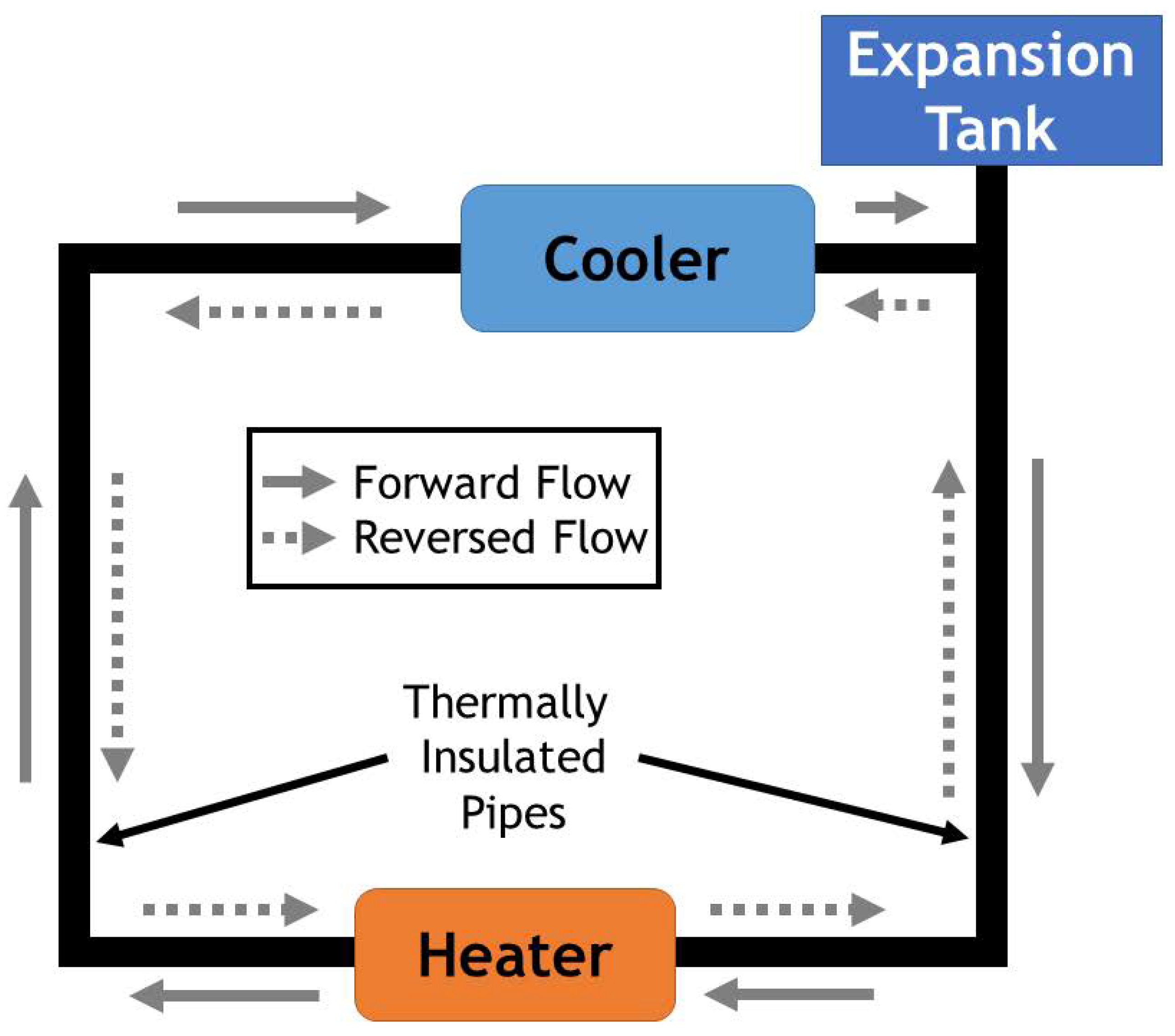
2. Description of the Numerical Model

Figure 1 depicts a schematic diagram for the physical process of a natural circulation loop (NCL) system. The circulation loop is 4 m in length with the inner tube diameter of 30 mm; an electrical heater of length 400 mm is placed in the middle of the bottom limb of the loop, which acts as the heat source to the NCL system. An annular-type cooler, with a length of 600 mm, is placed with a 100 mm offset on the upper horizontal arm of the loop to cool the loop fluid; this offset is necessary to start the simulation. Although detailed descriptions of the loop geometry, model construction and validation, and grid and time independence studies are reported in previous publications [18,19,20], a concise description of the model equations is provided in this section for completeness of the paper and ease of readability. The nomenclature of the terms used in the development of equations is provided at the end of the paper.
The governing equations (e.g., conservation of mass, momentum, and energy) for the loop fluid flow, and coolant and wall temperatures are solved numerically. These equations, which are similar to those in earlier publications [18,19,20], are only briefly explained here. For example, the continuity, momentum, and energy equations are represented by Equations (1)–(3), respectively. Here the mass flux is denoted by G ( = ρ v ) and the fluid flow by the subscript ’ f l ’.
Conservation of mass (liquid phase):
ρ f l t + t ( G f l ) = 0
Conservation of momentum (liquid phase):
d G f l d t L l o o p = f G f l 2 2 ρ f l d i n L l o o p + v e r t i c a l l i m b s ρ f l g cos θ β a v ( T f l T r e f ) d z
The momentum equation is integrated over the entire loop to arrive at the current form of Equation (2), which shows the forces acting on the loop fluid. In Equation (2), the left-hand side represents the fluid inertia force, the first term on the right-hand side represents the friction force, and the second term represents the buoyancy force. The balance of these forces determines the magnitude and direction of the force due to the fluid flow inside the loop.
As seen below in the equations of dynamic energy balance for the loop fluid and the coolant (that is flowing inside the cooler in Figure 1), the first term on the left-hand side indicates the transient energy and the second term on the left-hand side is the convective heat transfer. The first term on the right-hand side is the conduction heat transfer and the second term on the right-hand side is the heat exchange due to convection.
Conservation of energy (liquid phase):
t ( ρ f l C p t f l ) + z ( G f l C p T f l ) = z k f l T f l z 4 h i ( T f l T w ) d i n
Conservation of energy (heat exchanger):
t ( ρ e x C p , e x T e x ) + z ( G e x C p , e x t e x ) = z k e x T e x z h e x A e x ( T w T e x ) v e x
In Equation (3), heat exchange takes place between loop fluid and loop wall; and, in Equation (4), heat exchange takes place between loop wall and coolant. Accordingly, the respective convective heat transfer coefficient is assumed for the loop fluid and the coolant.
Conservation of energy (heat exchanger tube wall):
t ( ρ w C p , w t w ) = z k w T w z + h i A i ( T f T w ) V w 1 ( h 0 + h r ) A 0 ( T w T a ) V w 1 + Q ˙ V w 2
In Equation (5), the left-hand term is the transient energy flow and the first term on the right-hand side is the conduction heat energy flow in the tube wall, while the second and third terms on the right-hand side are the flow of convective heat energy to and from the tube wall, respectively; and the fourth term on the right-hand side is the flow of exogenous (electrically heated) energy input. Therefore, if the entire apparatus except the heater and the cooler is perfectly thermally insulated from the environment (i.e., no heat transfer takes place between the loop wall and ambient), the net exogenous heat input is absent (i.e., Q ˙ = 0 ) for the loop except the heater and cooler. The loss of thermal energy from the heater and cooler to the environment is represented in the third term on the right-hand side of Equation (5) that has two parts: one is convective heat loss and the other is radiation heat loss, where h 0 and h r are the convective and (linearized) radiation heat transfer coefficients, respectively. When radiation is considered, the radiative heat transfer coefficient is computed as h r = 4 ε σ T a 3 , where ε = 0.8 and σ = 5.67 × 10 8 .
Several closure relations are needed to complete the governing equations of the numerical model. These closure relations are furnished in detail in the earlier work [18] and are only briefly presented here for completeness of the paper. For the numerical simulation, several correlations are used in computing: (i) the friction factor, (ii) the heat transfer coefficient between wall and loop fluid, (iii) the heat transfer coefficient between wall and coolant in the heat exchanger, and (those between the wall and air).
For evaluating the friction factor (f) the following correlations have been used:
f = 64 R e d , for R e d < 2300 ( Laminar )
f = 3.03 × 10 12 R e d 3 3.67 × 10 4 R e d 0.151 for 2300 < R e d < 4500 ( Transition )
f = ( 0.79 l n R e d 1.64 ) 2 , for R e d > 4500 ( Turbulent )
R e d is the Reynolds number based on the mass flux ( G f l ) generated by buoyancy effects given by: R e d = ( G f l d i n ) / μ f . The correlations used for determining fluid to wall heat transfer are listed below [35,36].
For the laminar flow:
N u d = 1.86 R e d 1 / 3 P r 1 / 3 d i n L l o o p 1 / 3 μ f l μ s 0.14 , for G z > 10
N u d = 3.66 , for G z 10
where the Graetz Number ( G z ) is defined as G z = ( π d i n ) / ( 4 L l o o p ) R e d P r , and P r being the Prandtl number.
For the transition and turbulent flow, the Nusselt number ( N u d ) is determined by the Petukhov correlation with Gnienlinski modification [35,36]:
N u d = ( f / 8 ) ( R e d 1000 ) P r 1 + 12.7 ( f / 8 ) 1 / 2 ( P r 2 / 3 1 )
where the friction factors are computed as in Equations (6)–(8). The heat transfer from tube wall to ambient for the riser and downcomer sections is evaluated by using the correlations for the vertical cylinders [35,36]:
N u l , c y l = C F × N u l
where
N u l = 2.8 l n 1 + 2.8 C 1 R a 1 / 4
R a = G r . P r = g β a v L H 3 ( T w T a ) ν 2 . v α
and
C F = 1.8 Φ l n ( 1 + 1.8 Φ )
Φ = L H / d 0 C l R a 1 / 4
The heat transfer from tube wall to ambient for the horizontal sections is estimated by the following correlation.
N u l = 0.6 + 0.387 R a 1 / 6 1 + ( 0.559 P r ) 9 / 16 8 / 27 2 , for 10 5 < R a < 10 12
The numerical model used in this paper was compared and validated with the experimental and numerical results in the previous publications [18,19,20]; therefore, a validation study is not repeated here for compactness of the paper.
NOTE:The governing equations of the NCL system have been solved by using a finite volume approach on a lumped parameter model. As such this model may not capture certain local phenomena arising from two-phase behavior and bubble formation. However, the lumped parameter approximation is reasonable in this case, because the average operating temperatures are well below the saturation temperature of the fluid.

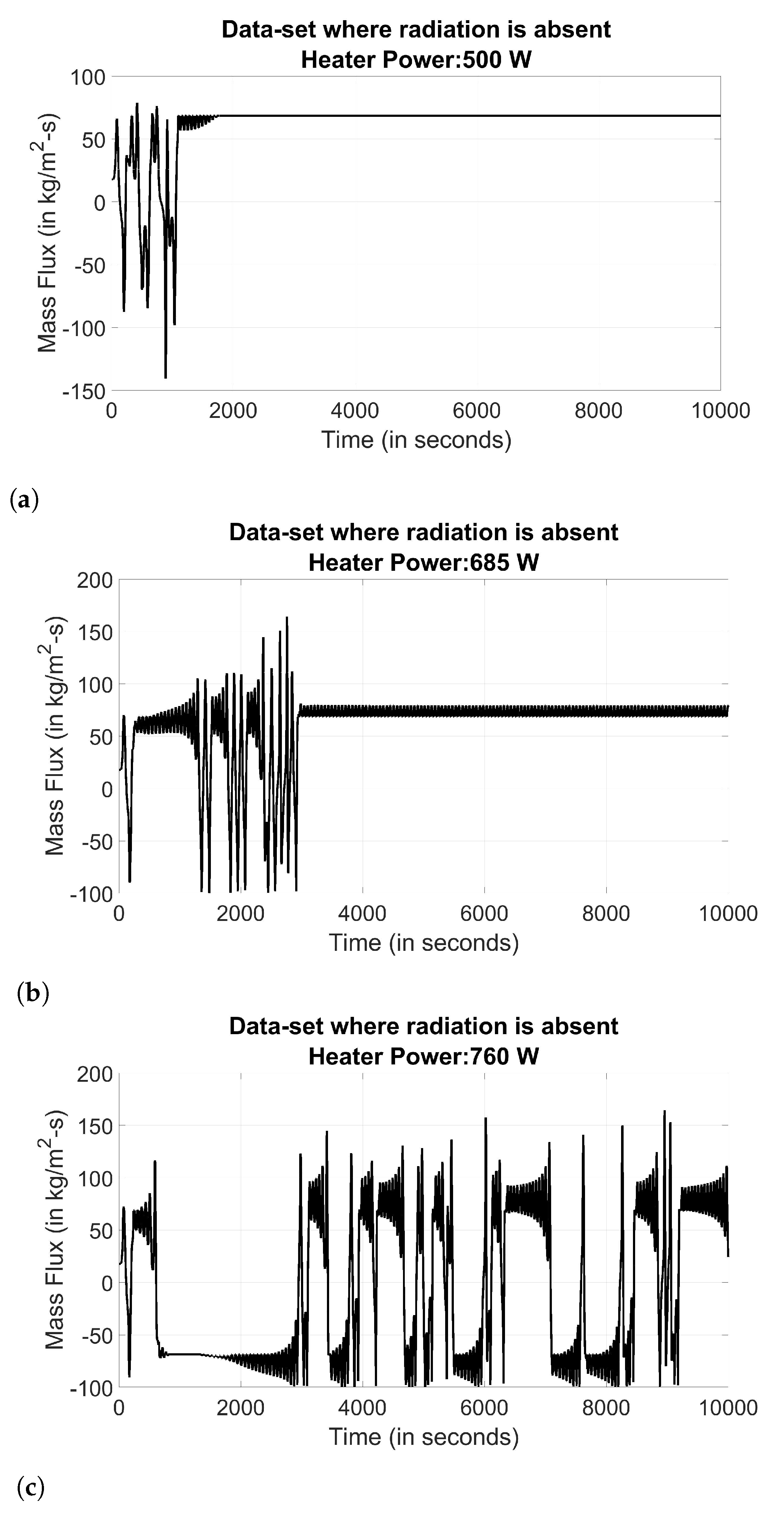
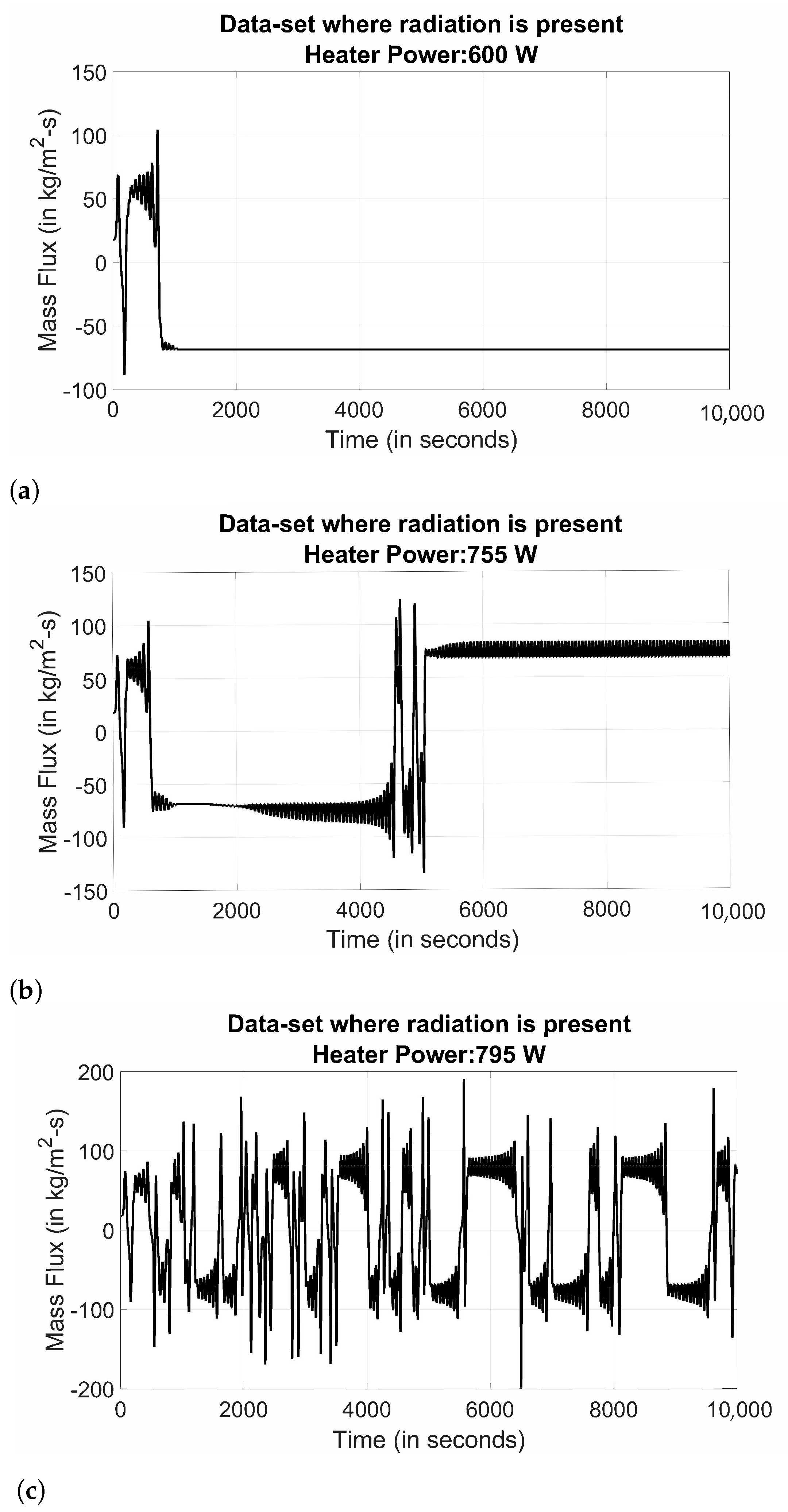
3. Numerical Results

In the first set of numerical simulation, radiation heat loss is ignored and accordingly, the parameter h r is set to zero in Equation (5). It is observed in the numerical simulation that the flow dynamics change with an increase in heater power. For relatively low heater power, the flow dynamics approximately exhibit a steady-state nature; as the heater power is gradually increased, the dynamic behavior first changes to an oscillatory nature and then, with further increase in the heater power, it exhibits flow-reversal [19], as seen in Figure 2.
The fluid flow in an NCL system is established by the temperature difference between its two vertical limbs: the riser (with a higher temperature) and the downcomer (with a lower temperature). The difference in temperature produces a density difference, which in turn produces the fluid flow to balance the buoyancy, friction and inertia forces. For a relatively low heater power, a steady unidirectional flow is seen in Figure 2a, and this region is said to exhibit a steady-state behavior. In this regime of operation, the flow dynamics remain unaltered as heater power is moderately increased, but the steady-state value of mass flux increases as the input power increases.
With a further increase in the heater input power, the flow velocity may become so high that sufficient time is not available for the fluid to be heated via heat transfer at the heater. Accordingly, the relatively cold fluid with higher density enters the riser section, and consequently, the buoyancy force is reduced, which causes a drop in the flow velocity. This, in turn, allows sufficient time for the fluid to get heated and consequently flow velocity increases due to the increase in the buoyancy force. This periodic change in flow velocity yields the oscillatory nature of the time series, as seen in Figure 2b and this regime is called oscillatory. In this regime, increase of the heater power keeps the flow dynamics oscillatory, which also increases the oscillation amplitude of the mass-flux.
With a still further increase in the heater power, the flow velocity becomes very high due to the high buoyancy force. This high flow velocity reduces the further residence time of the fluid in the heater and the cooler sections. Consequently, more of the relatively cold fluid (i.e., with higher density) enters the riser section, and relatively hot fluid (i.e., with lower density) enters the downcomer section. Therefore, similar to the oscillatory case, the temperature difference between the riser and the downcomer sections significantly decreases; and when this temperature difference approaches zero, it causes the flow velocity to approach zero. Due to the inertia, however, fluid begins to flow in the opposite direction causing the flow to reverse. This is the reason behind the chaotic flow-reversal characteristics in the time series, as seen in Figure 2c and this region is said to be the flow-reversal regime. In this region, the flow dynamics is rather chaotic with frequent switching of the flow direction.
In the next set of numerical simulation, radiation heat loss is included (see Equation (5)); a similar behavior of flow dynamics is observed, where the increase in the heater power causes the flow dynamics to change. Once again, relatively low heater power shows steady-state flow; and an increased heater power first changes to the oscillatory regime and then a further increase in heater power yields flow-reversal as seen in Figure 3. However, due to the radiation heat loss, the change-over points of flow dynamics (i.e., the value of heater power at which flow regimes change, are different as seen in Table 1. It has been observed during the simulations that the value of h r / h 0 , (i.e., the ratio of the radiative heat transfer coefficient and the convective heat transfer coefficient, both between the outer wall of the pipe and the ambient) averages in the vicinity of 0.40. This indicates that for the same operating condition, with radiative heat transfer can significantly change the heat transfer in the system, and the regime of operation.
A similarity between the trends in the cases with and without radiation is apparent. It is also noted that the duration of the initial transience is not constant. Another interesting point is seen in Figure 3b, where the system undergoes a bifurcation within the 4000–5000 s window, while retaining the same regime of operation. This is possibly an outcome of the inherent nonlinearity in the system.

4. Mathematical Theory

This section presents the essential background for construction of probabilistic finite state automata (PFSA) (see Section 4.1) and D-Markov machines (see Section 4.2), which belong to the class of symbolic time-series analysis (STSA) [21,22,23,24].

4.1. Probabilistic Finite State Automata

Using a Symbolic Time-Series Analysis (STSA) approach, the measured signal is converted to a symbol string by first partitioning (or quantizing) the signal and then followed by its symbolization. Thus, the signal space is converted into a finite number of partitioned cells, where the number of cells is identically equal to the cardinality | 𝒜 | of the (symbol) alphabet A . A symbol from the alphabet A is assigned to a point in the signal, corresponding to the cell to which it belongs [37,38]; details are given in [24]. The following definitions, which are available in standard literature (e.g., [23,24]), are recalled for completeness of the paper.
Definition 1.
A finite state automaton (FSA) G, with a deterministic algebraic structure, is defined as a triplet A , Q , δ where:
  • A is a (nonempty) finite alphabet, i.e., its cardinality | A | is a positive integer.
  • Q is a (nonempty) finite set of states, i.e., its cardinality | Q | is a positive integer.
  • δ : Q × A Q is a state transition map.
Definition 2.
A symbol block, or ’word’, is a finite-length string of symbols (belonging to the alphabet A ), where the length of a word w s 1 s 2 s is | w | = , with every s i A , and the length of the empty word ϵ is | ϵ | = 0 . The parameters of the FSA are extended as:
  • The set of all words including the empty word ϵ, constructed from symbols in A , is denoted as A 🞰 .
  • The set of all words, whose suffix (respectively, prefix) is the word w, is denoted as A 🞰 w (respectively, w A 🞰 ).
  • The set of all words of (finite) length ℓ is denoted as A , where ℓ is a positive integer.
Remark 1.
A symbol string (or word) is generated from a (finite-length) time series by symbolization.
Definition 3.
A probabilistic finite state automaton (PFSA) K is defined as a pair ( G , π ) , where:
  • The deterministic FSA G is called the underlying FSA of the PFSA K.
  • The probability map π : Q × A [ 0 , 1 ] is called the morph function (also known as symbol generation probability function) that satisfies the condition: s A π ( q , s ) = 1 for all q Q which can be converted to a | Q | × | A | morph matrix Π
  • The state transition probability mass function κ : Q × Q [ 0 , 1 ] is constructed by combining δ and π, which can be structured as a | Q | × | Q | state transition probability matrix T . In that case, the PFSA can also be described as the triple J = A , Q , T .
Equivalently, a PFSA is a quadruple K = A , Q , δ , π .

4.2. D-Markov Machines

The PFSA model of in a D-Markov machine generates symbol strings { s 1 s 2 s : N + and s j A } , where N + { 1 , 2 , 3 , } , on the underlying Markov process. In the construction a D-Markov machine it is primarily assumed that the generation of a symbol depends only on a finite history of at most D consecutive symbols, i.e., a symbol block of length not exceeding length D. A D-Markov machine [24] is defined as follows.
Definition 4.
A D-Markov machine [23] is a PFSA in the sense of Definition 3 which generates symbols that solely depend on the (most recent) history of at most D consecutive symbols, where the positive integer D is called the depth of the machine. Equivalently, a D-Markov machine is a statistically stationary stochastic process S = s 1 s 0 s 1 , where the probability of occurrence of a new symbol depends only on the last consecutive (at most) D symbols, i.e.,
P [ s n s n D s n 1 ] = P [ s n s n D s n 1 ]
Consequently, for w A D (see Definition 2), the equivalence class A 🞰 w of all (finite-length) words, whose suffix is w, is qualified to be a D-Markov state that is denoted as w.
For the PFSA method, there are primarily four choices as listed below:
  • Alphabet size ( | A | ): To separate out the regimes in the feature space, a larger alphabet size is preferred but more data is required for training the model. For the purpose of this paper, an alphabet size | A | = 6 was sufficient.
  • Partitioning Method: Maximum entropy partitioning (MEP) [24,37,38], which is a commonly used partitioning technique, has been chosen in this paper.
  • Depth (D) in the D-Markov machine: Sometimes, a higher value of the Markov depth D may lead to better results. However, this comes at the expense of increased computational time, due to larger dimension of the space and the need for more training. In this work, D = 1 has been chosen to keep lower word lengths and smaller PFSAs which leads to faster training and testing.
  • Choice of Feature: The feature needs to be one that best captures the nature (e.g., texture) of the signal. The morph matrix Π (which for D = 1 is identical to the state transition matrix T ) has been chosen as the feature, because it is easily computed and captures the pertinent dynamics embedded in the signal.
NOTE:In this paper, raw data are normalized before partitioning, ensuring that the data has a zero mean and unit variance prior to partitioning. However, a global partition is not used, i.e., the partitions are recomputed for every window. This is necessary as the data have varying amplitudes, as seen in Figure 2 and Figure 3.

4.3. Hidden Markov Modeling for Classification

Hidden Markov modeling (HMM) has found applications in multiple problems and has shown high classification accuracy in almost all of them [39]. Thus, HMM has been chosen as the baseline to evaluate the performance of the (computationally much less expensive) PFSA-based method. The details of hidden Markov modeling (HMM) are extensively reported in technical literature (e.g., [40]), and thus, only the key concepts are reiterated here for completeness of the paper. For the detailed mathematics, the readers are requested to follow the references.
HMMs are capable of learning and representing long-range dependencies between observations, with underlying models that are assumed to be probabilistic functions of the hidden states [41]. A time series of T continuous (real-valued) observations with a discrete-time representation as a data string Y = { y 1 , y 2 , , y T } , assuming a first-order Markov property [42] over the observations, has a joint probability density function of Y obtained as:
p ( Y ) = p ( y 1 ) t = 1 T 1 p ( y t + 1 | y t )
HMMs have been widely used for speech recognition [30], time-series classification [31] and, more recently, the classification of chaotic data [33]. HMMs essentially belong to a class of doubly embedded stochastic processes, with a latent stochastic process of hidden state evolution. This evolution cannot be directly observed, but can be inferred by observing another stochastic process that produces the sequence of observations [40], which capture the long-range dependencies among observations and enables the usage of HMMs as black-box density models on observation sequences. The primary difference between the HMM and the standard Markov model is that the HMM does not directly assume the Markov property (i.e., conditional dependence on the states and being independent of each other) for the observations themselves. Rather, the hidden state sequence Z = { z 1 , z 2 , , z T } is assumed to follow Markovian dynamics, i.e., given the current state z t , the future state z t + 1 is independent of all the states prior to time instant t.
Formalizing the mathematical structure, for a string of observations { y 1 , , y T } assumed to be generated by a hidden state sequence { z 1 , , z T } , a HMM is constructed as a triplet λ = { A , B , π } [40], where:
(1)
A [ a i j ] is the | N | × | N | state-transition probability matrix, where | N | is the finite number of hidden states belonging to the set N of hidden states:
a i j = p ( z t + 1 = q j | z t = q i ) : q i , q j N
where j a i j = 1 i and a i j 0 i , j .
(2)
B [ b j ( y t ) ] is the probability density of the observation given the state:
b j ( y t ) = p ( y t | z t = q j )
(3)
π [ π i ] is the probability distribution of the initial state z 1 : π i = p ( z 1 = q i ) , where π is a 1 × | N | vector with i π i = 1 | N | = 1 and π i 0 i .
Following a model λ , the corresponding joint probability distribution of states and observations has the form:
p ( Y , Z ) = p ( z 1 : T ) p ( y 1 : T | z 1 : T ) = p ( z 1 ) t = 1 T 1 p ( z t + 1 | z t ) t = 1 T p ( y t | z t )
During the training phase, a commonly used expectation maximization (EM) procedure, called the Baum-Welch algorithm [40], is used to learn HMM models belonging to each of the K classes. The Baum-Welch algorithm [40] is applied to train the HMM triplet (see above) λ k which is a triplet λ k = { A k , B k , π k } [40], k = 1 , , K , where A k , B k , and π k are defined similarly as A, B, and π for each class k. The procedure is repeated for each of the K classes.
During the testing phase, data from an unknown class are provided as inputs to the algorithm. Given this observational sequence and the HMM models for each of the K classes, λ k = { A k , B k , π k } , the problem is to find the most likely model associated with this data. This is expressed as:
p ( Y | λ k ) = Z p ( Y | Z , λ k ) p ( Z | λ k ) = z 1 , z 2 , , z T π z 1 b z 1 ( y 1 ) a z 1 z 2 b z 2 ( y 2 ) a z T 1 z T b z T ( y T )
which is obtained by using the Forward Procedure [40] to compute the log-likelihood ( L k ) of the given time-series data belonging to each of the K classes. The final decision, as to which class the unknown data belongs, is made by selecting the class with the largest log-likelihood as follows:
Selected Class = argmax k { 1 , 2 , , K } L k
A continuous HMM formulation has been used in this paper, which uses a Gaussian mixture model with M = 2 Gaussian components to model the emission and there are N = 4 hidden states. Detailed algorithms for HMM are available in [40,41].

5. Problem Formulation and Algorithm Development

Referring to Figure 2 and Figure 3, it is seen that the operational regimes of the NCL system, namely steady-state (SS), oscillatory (OL) and flow-reversal (FR), are characterized by the textures of respective fluid flow. The primary objective here is to build a data-driven classifier that would be capable of identifying these three regimes, while the second objective is to determine how early the decisions of classification can be made, given that the duration of initial transience varies for individual operating conditions, irrespective of the final regime. This phenomenon occurs due to the nonlinearity of the NCL system, which may not have a fixed bifurcation point.

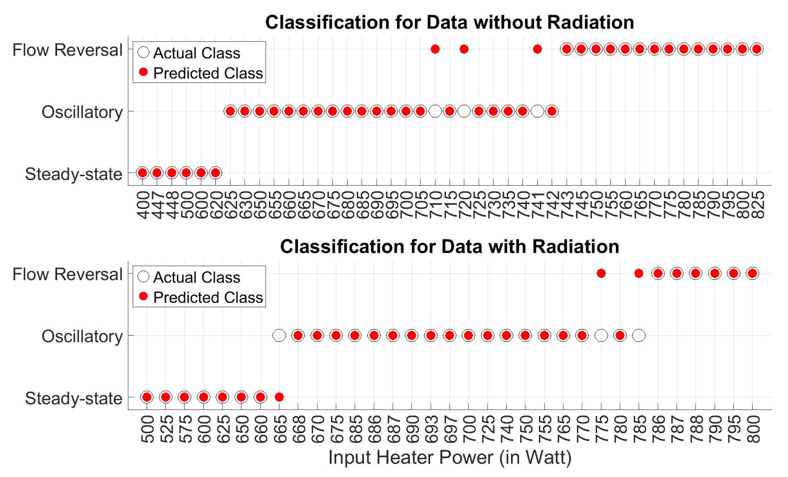
5.1. Regime Classification

This subsection develops PFSA-based algorithms for classification of NCL system regimes; the objective here is to classify the system regime within a specified time limit, which is taken to be 7200 s (2 h) in this paper.
During the training phase, the time series at a given operating condition is windowed, with window length W L and window skip W S , where having W S < W L implies that the windows do overlap. For each window, a PFSA feature (i.e., the morph matrix Π as described in Section 4.2) is generated, and the mean morph matrix is computed for the entire time series. Once all the time-series data from a given regime are observed, and their mean morph matrices are generated, yet another mean of the morph matrices is taken to arrive at the final representative morph matrix for each regime, which yields this yields Π S S , Π O L and Π F R .
During the testing phase, the time series (that belongs to an unknown) is windowed in the same manner and a final morph matrix for the entire time series, Π T S , is computed by averaging as described above. The final decision of which regime the test time series belongs to, is made as follows:
Selected Class = argmin c { S S , O L , F R } | | Π T S Π c | |
It is noted that the above approach to training a PFSA is different from those seen in the standard PFSA-based classification literature (e.g., [43]). This modified approach is needed because the problem here is to capture the evolving nature and not just to classify a statistically stationary time series.
For the HMM-based classification, the time series in its entirety is used for training of the three HMMs corresponding to each of the regimes. A windowed formulation is not needed here because the HMM method inherently learns long-term dependencies. In the testing phase of HMM, the log-likelihood (L) of the time series for each of the three regimes is computed, and the final classification decision is made by following Section 4.3 as:
Selected Class = argmax c { S S , O L , F R } L c

5.2. Identification of System Nature

The algorithm described in the subsection above allows for detecting the regime of operation only after observing the time series for a considerable amount of time, because the region of observation is kept identical for both training and testing. This region of observation needs to be relatively large, because the final dynamics may evolve late in the operation and, for appropriate training, it needs to be observed and included in the learning of the system dynamics.
However, for appropriate prognosis of a continuously evolving plant, it is desirable to identify any change in the regime of operation as soon as possible. As mentioned before, the initial transience is rather long and may vary significantly. This makes it difficult to specify an early fixed point by which the system would settle into its final regime. In this subsection, a methodology is proposed to attempt to make this identification as fast as possible.
In the PFSA method, the training of the morph matrices (i.e., Π S S , Π O L or Π F R ) of the regime is identical to that of the method described in the previous section. During testing, however, the region of observation is varied from a small region (of length W L ) to the entire region considered in the algorithm described in the previous subsection. Accordingly, the morph matrix evolves and the endeavor is to see how fast the regime can be correctly identified using Equation (23).
Similarly, for the HMM method, the HMM models for each regime are trained identically to the previous section, and the transient identification is done for a varying region of observation as in the PFSA method.

6. Results and Discussions

As stated in Section 3, two datasets are generated from the numerical model described in Section 2. One dataset is an ensemble of 43 time series, consisting of the following contents: 6 from the steady-state regime, 23 from the oscillatory regime, and 14 from the flow-reversal regime, where the effects of radiation heat loss are neglected. In the second dataset, the effects of radiation heat loss is considered, which consists of 33 time series with the following contents: 7 from the steady-state regime, 20 from the oscillatory regime, and 6 from the flow-reversal regime. Each of the above time series is typically run until over 10,000 s (i.e., ∼2.7 h) of operation. The initial transience ranges from anywhere between 1000 s to 3000 s. Thus, the total region of observation is taken to be from 1000 s (to preclude observing too much of the transient data) till 9000 s, by which time (e.g., 7200 s) the NCL system is expected to arrive at the final regime of operation. The PFSA method uses the following windowing parameters: window length W L = 600 s and window skip W S = 60 s.

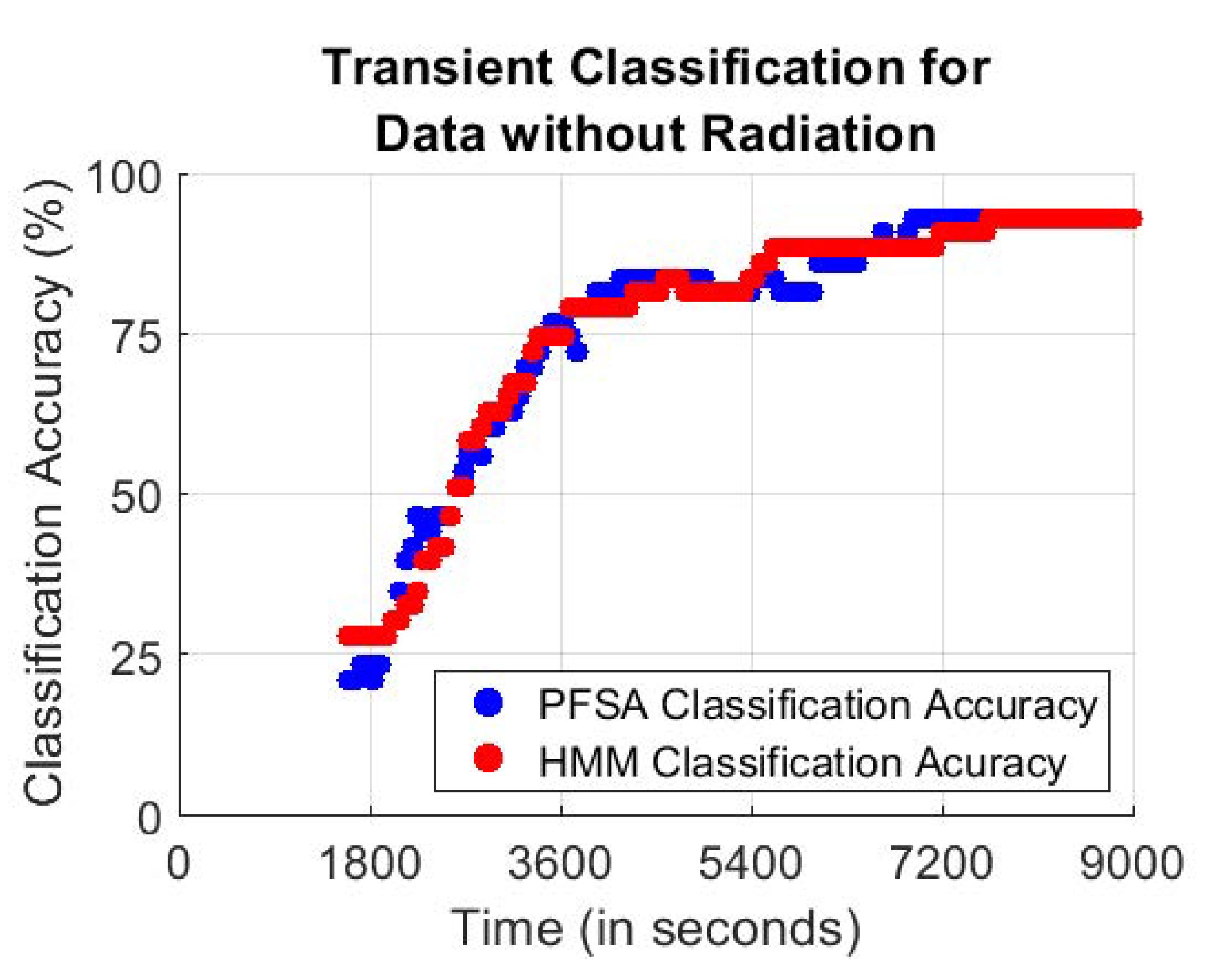
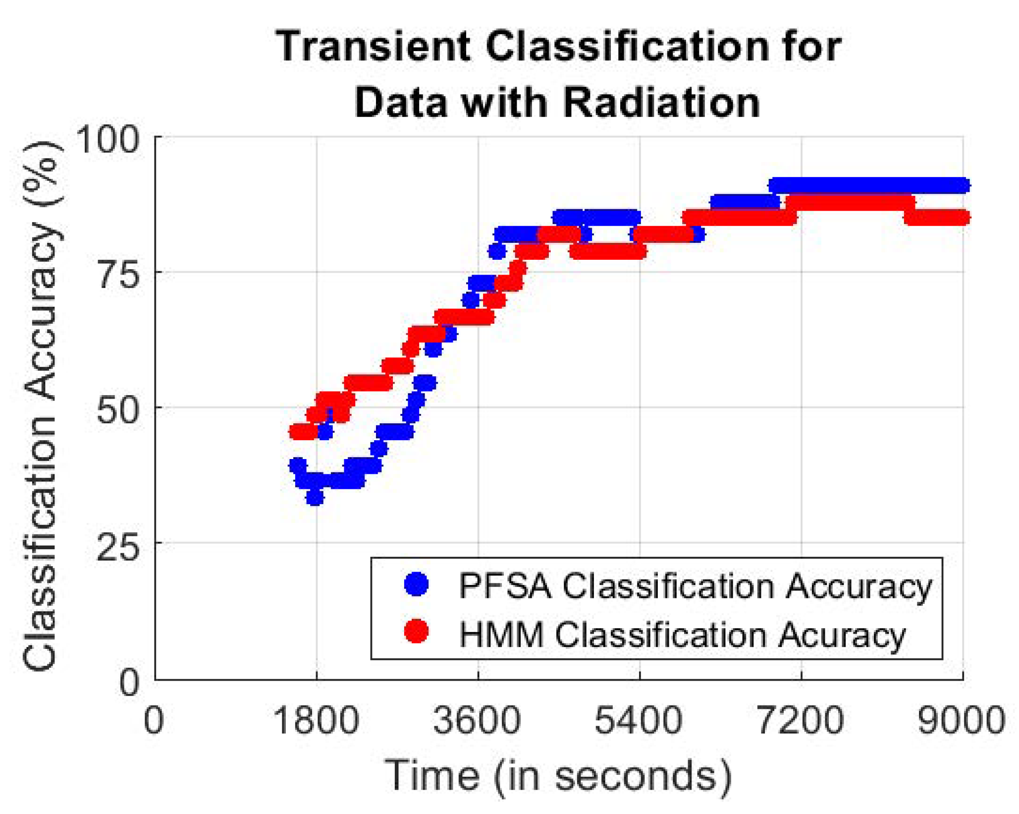
6.1. Classification Accuracy

To test the efficacy of the regime classification algorithm, described in Section 5.1, the PFSA models are trained exclusively using the no-radiation-loss data, where the dataset is split into 50% for training for both PFSA (i.e., morph matrices Π S S , Π O L and Π F R ) and HMM, and the remaining 50% are used to test the performance of the respective algorithms of PFSA and HMM. Each of the two confusion matrices in Table 2 shows the average accuracy of classification over 20 trials after until 7200 s; the training and testing sets are randomly chosen for each trial for both methods. The total error (i.e., percentage of total number of time series classified incorrectly) is 10.71% for the PFSA method and 18.57% for the HMM method.
Remark 2.
Some combinations of test-train data split have yielded a total error of 0% for the PFSA method and 4.57% for the HMM method. The morph matrices and HMM models for each regime corresponding to these trials have been saved as the optimal trained representative PFSAs (morph matrices)/HMMs for the three regimes. These trained PFSAs /HMMs were once again used to classify all 43 datasets of time series in the no-radiation dataset, including both the training and testing data. The resulting confusion matrices for both the methods are listed in Table 3, and the total error is seen to be ∼6.98% for both PFSA and HMM methods.
The next step is to check whether the PFSAs and HMMs trained on data, with no radiation heat loss, are capable of successfully classifying simulated data generated by including the radiation heat loss.
Table 4 lists the confusion matrix reporting the classification accuracy of all (33) time series incorporating radiation heat loss by using the PFSAs/HMMs that are optimally trained with the no-radiation data.
Good classification accuracy is seen in Table 4 for the PFSA method, with a total error of 9.09%, and an error of 15.15% for the HMM method. Thus, the PFSA method apparently captures the system dynamics modestly better than the HMM method and the results do not strongly depend on the actual system operating conditions. The charts of Figure 4 show the classification accuracy of the optimal PFSAs for the datasets, with and without radiation heat loss. It is concluded that the PFSA algorithm is generally accurate, with very few time-series misclassifying the regimes and these misclassifications generally arise near the change points. The HMM method too presents largely similar results, as seen in Figure 5.

6.2. Computation Overhead

Table 5 compares the training and testing times of PFSA-based and HMM-based classification, where the individual computation times are calculated as an average of 20 independent trials using the total length of time series. It is seen that training and testing times for PFSA (with the parameters described in Section 4.2) is much lower than those for HMM. The rationale is that the PFSA algorithm is computationally very fast in both training and testing due to its non-iterative and algebraic construction, whereas the HMM algorithm is iterative and has a more complex mathematical construction as outlined in Section 4.3. It is concluded that on average, the PFSA method is of comparable accuracy as the HMM method at a small fraction of the computational cost, especially during training (e.g., with almost two orders of magnitude reduction in the training time).
NOTE:All the computations in this paper have been conducted using MATLAB PFSA codes by the authors (https://github.com/Chandrachur92/PFSA (accessed on 1 March 2021)) with Murphy’s [41] Hidden Markov Model (HMM) Toolbox for MATLAB (https://www.cs.ubc.ca/~murphyk/Software/HMM/hmm.html (accessed on 1 March 2021)). The computations have been conducted serially on a single core processor of a DELL Precision Tower 7910 Workstation running an Intel® Xeon® E5-2670 CPU.

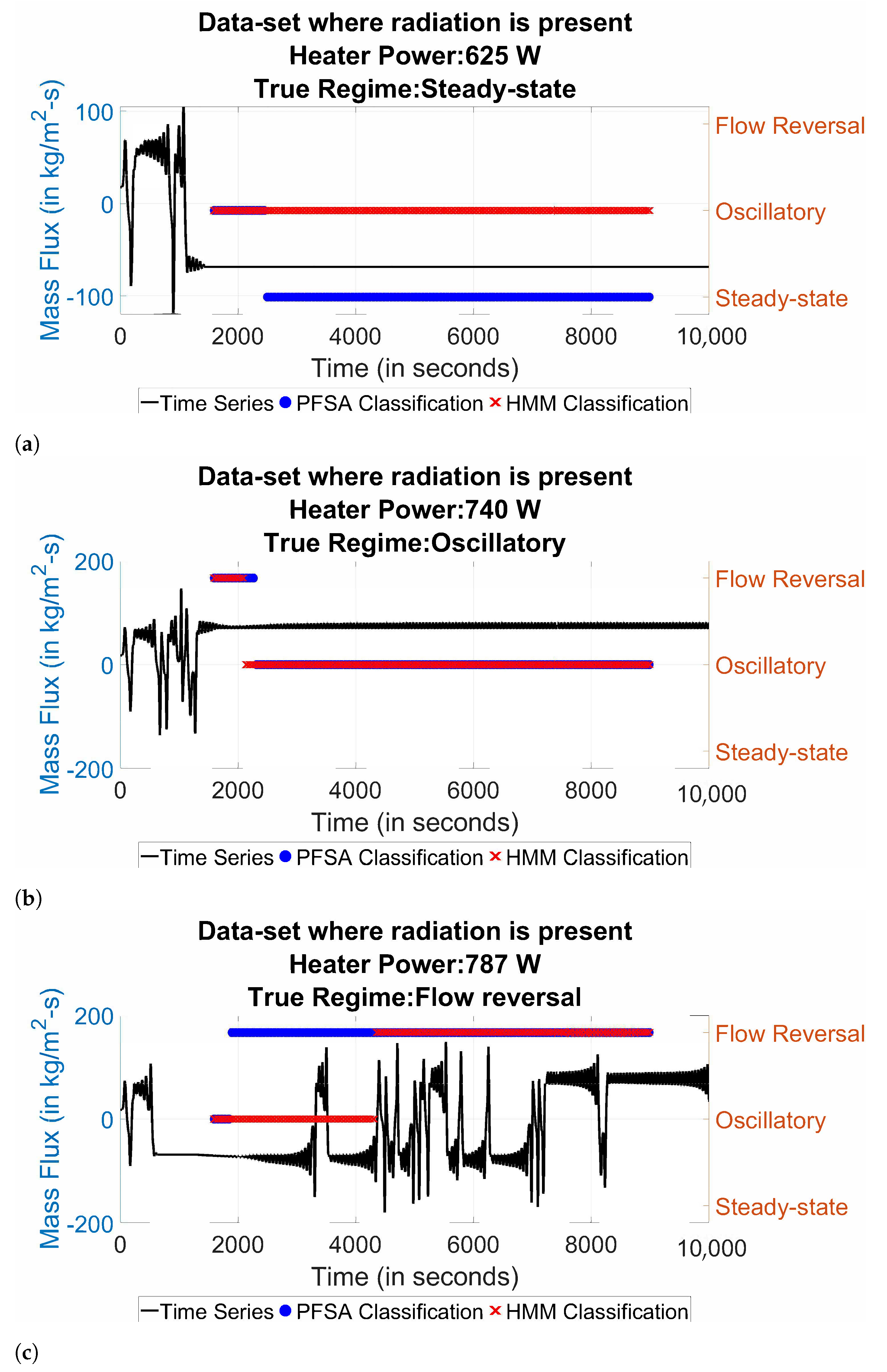
6.3. Efficacy of Identification/Classification

Although the PFSA algorithms (as well as the HMM algorithms serving as a baseline) produce good accuracy in identifying the regime of operation in the simulated NCL system, the classification occurs after observing 9000 s (i.e., 2.5 h) of data; this is not adequate for prognosis or control of the NCL system. Therefore, from an operational perspective, it is desirable to maintain the system under the steady-state operating condition and may be allowed to go into the oscillatory regime under extraneous circumstances. Nevertheless, it is not desirable to operate the NCL system in the chaotic flow-reversal regime, which causes a sharp degradation in the heat transfer characteristics of the heater and cooler (see Figure 1). Thus, the operating regime of an evolving NCL operation should be assessed as soon as possible to take necessary corrective actions whenever a tendency to go into the flow-reversal regime is observed.
The methodology proposed in Section 5 is used to test the algorithms for early assessment of the operational regime. This PFSA-based procedure is called transient classification, wherein at any point in time in the evolution of the NCL system characteristics, the morph matrix for the time series is obtained only by using the data available at that point (i.e., the beginning of the current time epoch). The classification proceeds as described in Equations (23) and (24). The earlier the algorithms can identify the final regime, the better it is.
For comparison of transient classification using PFSA and (baseline) HMM methods, Figure 6 and Figure 7 respectively exhibit the profiles of classification accuracy as a function of the time epochs for no-radiation-heat-loss and radiation-heat-loss datasets. It is noted that the classification at any point involves only data observed prior to it to maintain causality. The first identification occurs at ∼1600 s, because the first ∼1000 s are ignored (due to initial transience) and the window length needed to be observed is 600 s.
It is seen in Figure 6 and Figure 7 that the initial transient region (i.e., first ∼3000 s, including the initial transience) does not allow for good accuracy of identification (i.e., classification) using either PFSA or HMM. However, the accuracy almost monotonically increases as more data are observed, with almost 90% accuracy observed at the 7200 s mark using the PFSA method with HMM performance being slightly inferior; and an accuracy of greater than 75% after about merely 3600 s (slightly later for the HMM method on the data with radiation).
Although Figure 6 and Figure 7 provide a qualitative idea of how well the algorithms work at identifying the eventual regime of operation of the NCL system, a true evaluation of the method would be to study the time series individually. This is necessary because the initial transience may vary significantly for each case and that causes an apparent misclassification. Figure 8 and Figure 9 exhibit six representative time-series, in which three are form the no-radiation dataset and the remaining three are from the dataset with radiation, corresponding to each of the three regimes. In it, the identified regime using either method is superimposed to show how the proposed algorithm can identify the eventual regime of operation.
It is seen in Figure 8 and Figure 9 that after the initial transient region, the PFSA method can correctly identify the final regime of operation quite ahead of time. In fact, in both Figure 8b and Figure 9b, it is seen that the PFSA method is also capable of identifying the imminent change into the oscillatory regime long before the signal texture changes significantly, while the HMM method makes an accurate identification because of the transient phase itself. It is also interesting to note that although a bifurcation occurs in the 6000–8000 s window in Figure 8b, both PFSA and HMM are still able to correctly classify the ongoing system regime to be oscillatory. Similarly, in Figure 9c, the transition into the flow-reversal regime is preceded by both PFSA and HMM by detecting the imminent change. In Figure 8c, however, both PFSA and HMM initially mis-detect the system to be in the oscillatory regime, but later classifies it as the flow-reversal regime with the PFSA method identifying the change very early while the HMM method takes longer to make the correction. In Figure 9a, it is seen that the HMM method completely mis-classifies the steady time series to be oscillatory until 9000 s.
In view of the above observations, it is reasonable to conclude that the PFSA method is capable of early identification of the final regime of operation of the NCL system, and outperforms the (baseline) HMM method in many cases.

7. Summary, Conclusions, and Future Work

This paper has developed a supervised method to classify/identify the operational regimes of natural circulation loop (NCL) systems. The underlying algorithms are built upon the theory of probabilistic finite state automata (PFSA), where ensembles of time-series data have been generated from a previously validated numerical simulator of an experimental NCL system. Two datasets have been generated from the simulator: one where no radiation heat loss is included in the computation and the other one with radiation heat loss. The exclusion of radiation heat loss changes the regime transition-points, i.e., the heater power at which the system switches from a steady-state to an oscillatory regime of operation and then again from an oscillatory to a flow-reversal regime.
The proposed PFSA method is shown to be capable of classifying the regime of operation with good accuracy when tested with a sufficient length of dynamically evolving data. The PFSA method is also effective for identifying the regimes of operation, where the NCL system eventually settles down. This prediction capability enables prognosis of the NCL system and this knowledge can be used for decision and control of the NCL system. The PFSA method shows good accuracy even though NCL systems are nonlinear and (possibly) chaotic, leading to large variations in the system characteristics in independent operations.
The performance of PFSA has been compared to that of hidden Markov modeling (HMM) [40] which has served as a baseline method in this investigation. Although extensive test results demonstrate that the accuracy of regime identification/classification is comparable for PFSA and HMM, the computational time to test and train the HMM algorithm is significantly larger than that for the PFSA algorithm. It is concluded from the observed results that PFSA is apparently more suitable than HMM for solving the problem of regime identification/classification in NCL systems.
Although there are many areas of theoretical and experimental research, which must be investigated before the proposed PFSA method can be implemented in real-life applications, the following topics of future research are suggested to be pursued immediately.
(1)
Investigation of the efficacy of the PFSA algorithms using data from other experimental and industrial NCL systems and more simulations with varying geometry parameters.
(2)
Enhancement of the PFSA algorithms to accommodate smaller data window lengths (i.e., faster detection and identification of regimes).
(3)
Investigation of other regime identification/classification methods, such as different configurations of neural networks.
(4)
Quantitative analysis of the effects of radiative and convective heat transfer on operational characteristics of NCL systems.

Author Contributions

Conceptualization, C.B. and A.R.; methodology, C.B. and A.R.; software, C.B.; formal analysis, C.B.; model preparation and validation, C.B., R.S. and A.M.; data curation, R.S.; writing—original draft preparation, C.B.; writing—review and editing, ALL AUTHORS; funding acquisition, A.R. and A.M. All authors have read and agreed to the published version of the manuscript.

Funding

The first author thanks Indo-US Science and Technology Forum (IUSSTF) for granting the Research Internship for Science and Engineering (RISE) scholarship for collaboration between Pennsylvania State University (PSU) and Jadavpur University (JU). All authors acknowledge SPARC, MHRD, Govt. of India for supporting collaboration between PSU and JU through its Project No. P1065. The work reported here has also been supported in part by the U.S. Air Force Office of Scientific Research (AFOSR) under Grant No. FA9550-15-1-0400 in the area of dynamic data-driven application systems (DDDAS).

Data Availability Statement

The data presented in this study are available on request from the corresponding author.

Conflicts of Interest

The authors declare no conflict of interest. The funders had no role in the design of the study; in the collection, analyses, or interpretation of data; in the writing of the manuscript, or in the decision to publish the results.

Abbreviations

The following abbreviations are used in this manuscript:
A i Internal surface area of the loop through which heat transfer takes place area (m2)
A e x Surface area through which heat transfer takes place in the cooler (m2)
A 0 Surface area through which heat loss takes place to the ambient (m2)
C p Specific heat of fluid at constant pressure (J/kg· K)
C p , w Specific heat of wall at constant pressure (J/kg· K)
C p , e x Specific heat of coolant at constant pressure (J/kg· K)
d i n Internal loop diameter (m)
d 0 Outer loop diameter (m)
d z Change in length (m)
fFriction factor
gGravitational acceleration (m/s2)
G f Loop fluid mass-flux (kg/m 2 · s)
G e x Coolant mass-flux (kg/m 2 · s)
G r Grashof number
G z Graetz number
h i Heat transfer coefficient between the fluid and wall (W/m 2 · K)
h 0 Heat transfer coefficient between wall and ambient (W/m 2 · K)
h r Radiation heat transfer coefficient (W/m 2 · K)
h e x Heat transfer coefficient between wall and coolant (W/m 2 · K)
k f Thermal conductivity of the fluid (W/m· K)
k w Thermal conductivity of the wall (W/m· K)
k e x Thermal conductivity of heat exchanger (W/m· K)
L l o o p Total loop length (m)
L H Loop height (m)
N u Nusselt number
P r Prandtl number
QHeat input (W)
R a Rayleigh number
R e d Reynolds number
tTime (s)
T f Temperature of fluid (°C)
T w Loop wall temperature (°C)
T e x Coolant temperature (°C)
T r e f Reference temperature (°C)
T a Ambient temperature (°C)
v f The component of the fluid velocity in the z–direction (m/s)
V w 1 Volume of the wall except heater and cooler section (m3)
V w 2 Volume of the wall in the heater section (m3)
V e x Volume of the heat exchanger (m3)
β a v Thermal volumetric expansion coefficient (K 1 )
μ f Dynamic viscosity of the fluid (kg/m· s)
μ s Dynamic viscosity of the fluid at the surface (kg/m· s)
ν Kinematic viscosity of the fluid (m 2 /s)
ρ f Fluid density (kg/m 3 )
ρ w Wall density (kg/m 3 )
ρ e x Coolant density (kg/m 3 )

References

  1. Vijayan, P.; Austregesilo, H.; Teschendorff, V. Simulation of the unstable oscillatory behavior of single-phase natural circulation with repetitive flow reversals in a rectangular loop using the computer code ATHLET. Nucl. Eng. Des. 1995, 155, 623–641. [Google Scholar] [CrossRef]
  2. Vijayan, P. Experimental observations on the general trends of the steady state and stability behaviour of single-phase natural circulation loops. Nucl. Eng. Des. 2002, 215, 139–152. [Google Scholar] [CrossRef]
  3. Vijayan, P.; Sharma, M.; Saha, D. Steady state and stability characteristics of single-phase natural circulation in a rectangular loop with different heater and cooler orientations. Exp. Therm. Fluid Sci. 2007, 31, 925–945. [Google Scholar] [CrossRef]
  4. Misale, M.; Tagliafico, L. The transient and stability behaviour of single-phase natural circulation loops. Heat Technol. 1987, 5, 101–116. [Google Scholar]
  5. Misale, M.; Garibaldi, P.; Tarozzi, L.; Barozzi, G.S. Influence of thermal boundary conditions on the dynamic behaviour of a rectangular single-phase natural circulation loop. Int. J. Heat Fluid Flow 2011, 32, 413–423. [Google Scholar] [CrossRef]
  6. Misale, M. Experimental study on the influence of power steps on the thermohydraulic behavior of a natural circulation loop. Int. J. Heat Mass Transf. 2016, 99, 782–791. [Google Scholar] [CrossRef]
  7. Cammi, A.; Luzzi, L.; Pini, A. The influence of the wall thermal inertia over a single-phase natural convection loop with internally heated fluids. Chem. Eng. Sci. 2016, 153, 411–433. [Google Scholar] [CrossRef]
  8. Goudarzi, N.; Talebi, S. Heat removal ability for different orientations of single-phase natural circulation loops using the entransy method. Ann. Nucl. Energy 2018, 111, 509–522. [Google Scholar] [CrossRef]
  9. Desrayaud, G.; Fichera, A.; Lauriat, G. Two-dimensional numerical analysis of a rectangular closed-loop thermosiphon. Appl. Therm. Eng. 2013, 50, 187–196. [Google Scholar] [CrossRef]
  10. Krishnani, M.; Basu, D.N. Computational stability appraisal of rectangular natural circulation loop: Effect of loop inclination. Ann. Nucl. Energy 2017, 107, 17–30. [Google Scholar]
  11. Nayak, A.; Vijayan, P.; Saha, D.; Raj, V.V. Mathematical modelling of the stability characteristics of a natural circulation loop. Math. Comput. Model. 1995, 22, 77–87. [Google Scholar] [CrossRef]
  12. Der Lee, J.; Pan, C.; Chen, S.W. Nonlinear dynamic analysis of a two-phase natural circulation loop with multiple nuclear-coupled boiling channels. Ann. Nucl. Energy 2015, 80, 77–94. [Google Scholar]
  13. Luzzi, L.; Misale, M.; Devia, F.; Pini, A.; Cauzzi, M.T.; Fanale, F.; Cammi, A. Assessment of analytical and numerical models on experimental data for the study of single-phase natural circulation dynamics in a vertical loop. Chem. Eng. Sci. 2017, 162, 262–283. [Google Scholar] [CrossRef]
  14. Goyal, V.; Hassija, V.; Pandey, V.; Singh, S. Non-linear dynamics of single phase rectangular natural circulation loop. Prog. Nucl. Energy 2020, 130, 103530. [Google Scholar] [CrossRef]
  15. Elton, D.; Arunachala, U.; Vijayan, P. Investigations on the dependence of the stability threshold on different operating procedures in a single-phase rectangular natural circulation loop. Int. J. Heat Mass Transf. 2020, 161, 120264. [Google Scholar]
  16. du Toit, C.G. Fundamental evaluation of the effect of pipe diameter, loop length and local losses on steady-state single-phase natural circulation in square loops using the 1D network code Flownex. Therm. Sci. Eng. Prog. 2021, 22, 100840. [Google Scholar] [CrossRef]
  17. Dass, A.; Gedupudi, S. Numerical investigation on the heat transfer coefficient jump in tilted single-phase natural circulation loop and coupled natural circulation loop. Int. Commun. Heat Mass Transf. 2021, 120, 104920. [Google Scholar] [CrossRef]
  18. Saha, R.; Sen, S.; Mookherjee, S.; Ghosh, K.; Mukhopadhyay, A.; Sanyal, D. Experimental and numerical investigation of a single-phase square natural circulation loop. J. Heat Transf. 2015, 137, 121010. [Google Scholar] [CrossRef]
  19. Saha, R.; Ghosh, K.; Mukhopadhyay, A.; Sen, S. Dynamic characterization of a single phase square natural circulation loop. Appl. Therm. Eng. 2018, 128, 1126–1138. [Google Scholar] [CrossRef]
  20. Saha, R.; Ghosh, K.; Mukhopadhyay, A.; Sen, S. Flow reversal prediction of a single-phase square natural circulation loop using symbolic time series analysis. Sādhanā 2020, 45, 1–11. [Google Scholar]
  21. Daw, C.; Fenney, C.; Tracy, E. A review of symbolic analysis of experimental data. Rev. Sci. Instrum. 2003, 74, 915–930. [Google Scholar] [CrossRef]
  22. Dupont, P.; Denis, F.; Esposito, Y. Links between probabilistic automata and hidden Markov models: Probability distributions, learning models and induction algorithms. Pattern Recognit. 2005, 38, 1349–1371. [Google Scholar] [CrossRef]
  23. Ray, A. Symbolic dynamic analysis of complex systems for anomaly detection. Signal Process. 2004, 84, 1115–1130. [Google Scholar] [CrossRef]
  24. Mukherjee, K.; Ray, A. State splitting and merging in probabilistic finite state automata for signal representation and analysis. Signal Process. 2014, 104, 105–119. [Google Scholar] [CrossRef]
  25. Sarkar, S.; Chakravarthy, S.; Ramanan, V.; Ray, A. Dynamic data-driven prediction of instability in a swirl-stabilized combustor. Int. J. Spray Combust. Dyn. 2016, 8, 235–253. [Google Scholar] [CrossRef]
  26. Bhattacharya, C.; O’Connor, J.; Ray, A. Data-driven Early Detection of Thermoacoustic Instability in a Multi-nozzle Combustor. Combust. Sci. Technol. 2020, 1–32. [Google Scholar] [CrossRef]
  27. Ghalyan, N.F.; Ray, A. Symbolic Time Series Analysis for Anomaly Detection in Measure-invariant Ergodic Systems. J. Dyn. Syst. Meas. Control 2020, 142, 061003. [Google Scholar] [CrossRef]
  28. Jha, D.; Virani, N.; Reimann, J.; Srivastav, A.; Ray, A. Symbolic analysis-based reduced order Markov modeling of time series data. Signal Process. 2018, 149, 68–81. [Google Scholar] [CrossRef] [Green Version]
  29. Li, Y.; Jha, D.K.; Ray, A.; Wettergren, T.A. Information-Theoretic Performance Analysis of Sensor Networks via Markov Modeling of Time Series Data. IEEE Trans. Cybern. 2018, 48, 1898–1909. [Google Scholar] [CrossRef]
  30. Najkar, N.; Razzazi, F.; Sameti, H. A novel approach to HMM-based speech recognition systems using particle swarm optimization. Math. Comput. Model. 2010, 52, 1910–1920. [Google Scholar] [CrossRef]
  31. Oates, T.; Firoiu, L.; Cohen, P. Using dynamic time warping to bootstrap HMM-based clustering of time series. In Sequence Learning; Springer: New York, NY, USA, 2000; pp. 35–52. [Google Scholar]
  32. Ali, S.S.; Ghani, M.U. Handwritten Digit Recognition Using DCT and HMMs. In Proceedings of the 2014 12th International Conference on Frontiers of Information Technology, Islamabad, Pakistan, 17–19 December 2014; pp. 303–306. [Google Scholar]
  33. Bhattacharya, C.; Ray, A. Data-driven Detection and Classification of Regimes in Chaotic Systems via Hidden Markov Modeling. ASME Lett. Dyn. Syst. Control 2021, 1, 021009. [Google Scholar] [CrossRef]
  34. Mondal, S.; Bhattacharya, C.; Ghalyan, N.F.; Ray, A. Real-Time Monitoring and Diagnostics of Anomalous Behavior in Dynamical Systems. In Dynamics and Control of Energy Systems; Springer: Berlin/Heidelberg, Germany, 2020; pp. 301–327. [Google Scholar]
  35. Basu, D.N.; Bhattacharyya, S.; Das, P. Effect of heat loss to ambient on steady-state behaviour of a single-phase natural circulation loop. Appl. Therm. Eng. 2007, 27, 1432–1444. [Google Scholar] [CrossRef]
  36. Basu, D.N.; Bhattacharyya, S.; Das, P. Effect of geometric parameters on steady-state performance of single-phase NCL with heat loss to ambient. Int. J. Therm. Sci. 2008, 47, 1359–1373. [Google Scholar] [CrossRef]
  37. Rajagopalan, V.; Ray, A. Symbolic time series analysis via wavelet-based partitioning. Signal Process. 2006, 86, 3309–3320. [Google Scholar] [CrossRef] [Green Version]
  38. Subbu, A.; Ray, A. Space Partitioning via Hilbert Transform for Symbolic Time Series Analysis. Appl. Phys. Lett. 2008, 92, 084107. [Google Scholar] [CrossRef]
  39. Mor, B.; Garhwal, S.; Kumar, A. A Systematic Review of Hidden Markov Models and Their Applications. Arch. Comput. Methods Eng. 2020. [Google Scholar] [CrossRef]
  40. Rabiner, L.R. A tutorial on hidden Markov models and selected applications in speech recognition. Proc. IEEE 1989, 77, 257–286. [Google Scholar] [CrossRef]
  41. Murphy, K. Machine Learning: A Probabilistic Perspective, 1st ed.; The MIT Press: Cambridge, MA, USA, 2012. [Google Scholar]
  42. Bishop, C. Pattern Recognition and Machine Learning; Springer: New York, NY, USA, 2007. [Google Scholar]
  43. Bhattacharya, C.; Ray, A. Online Discovery and Classification of Operational Regimes from an Ensemble of Time Series Data. J. Dyn. Syst. Meas. Control 2020, 142, 114501. [Google Scholar] [CrossRef]
Figure 1. Schematic diagram of the NCL system.
Sci 03 00014 g001
Figure 2. Sample mass-flux variation time series in absence of radiation heat loss for (a) Steady-state, (b) Oscillatory, and (c) Flow-reversal regimes.
Sci 03 00014 g002
Figure 3. Sample mass flux variation time series in the presence of radiation heat loss for (a) Steady-state, (b) Oscillatory, and (c) Flow-reversal regimes.
Sci 03 00014 g003
Figure 4. Case-wise classification accuracy for both datasets (without and with radiation) for PFSA.
Sci 03 00014 g004
Figure 5. Case-wise classification accuracy for both datasets (without and with radiation) for HMM.
Sci 03 00014 g005
Figure 6. Transient classification accuracy over all data without radiation heat transfer for PFSA and HMM.
Sci 03 00014 g006
Figure 7. Transient classification accuracy over all datasets with radiation heat transfer.
Sci 03 00014 g007
Figure 8. Transient classification for time-series in absence of radiation heat loss using PFSA and HMM for regimes of: (a) Steady-state, (b) Oscillatory, and (c) Flow-reversal.
Sci 03 00014 g008
Figure 9. Transient classification for time-series with radiation heat loss using PFSA and HMM for regimes: (a) Steady-state, (b) Oscillatory, and (c) Flow-reversal.
Sci 03 00014 g009
Table 1. Heater power at which NCL regimes move from steady-state to Oscillatory regimes, and oscillatory to flow-reversal regimes when radiation loss is ignored/included.
Change-Point for
Steady-State to Oscillatory
Change-Point for
Oscillatory to Flow-Reversal
Without radiation heat loss625 W743 W
With radiation heat loss665 W786 W
Table 2. Confusion matrix showing the average (over 20 trials) classification accuracy of the time-series regime from the dataset with no radiation heat loss.
PFSA Method: Classified asHMM Method: Classified as
SSOLFRSSOLFR
Truly SS100%0073.33%16.67%10.00%
Truly OL079.55%20.45%1.82%76.82%21.36%
Truly FR00100%07.86%92.14%
Table 3. Confusion matrix showing the classification accuracy of the regimes from the dataset with no radiation heat loss using the optimally trained PFSA and HMM.
PFSA Method: Classified asHMM Method: Classified as
SSOLFRSSOLFR
Truly SS100%0083.33%16.67%0
Truly OL079.55%20.45%095.65%4.35%
Truly FR00100%07.14%92.86%
Table 4. Confusion matrices showing the classification accuracy of the 33 time-series regimes from the dataset with radiation heat loss.
PFSA Method: Classified asHMM Method: Classified as
SSOLFRSSOLFR
Truly SS100%0071.43%28.57%0
Truly OL5%90%5%5%85%10%
Truly FR00100%00100%
Table 5. Training and testing times: PFSA and HMM.
PFSAHMM
Training Time per Time Series (in ms)18.75252.89
Testing Time per Time Series (in ms)22.867.43
Publisher’s Note: MDPI stays neutral with regard to jurisdictional claims in published maps and institutional affiliations.

