Numerical Simulation of the Fractal-Fractional Ebola Virus

Abstract

In this work we present three new models of the fractal-fractional Ebola virus. We investigate the numerical solutions of the fractal-fractional Ebola virus in the sense of three different kernels based on the power law, the exponential decay and the generalized Mittag-Leffler function by using the concepts of the fractal differentiation and fractional differentiation. These operators have two parameters: The first parameter $\rho$ is considered as the fractal dimension and the second parameter k is the fractional order. We evaluate the numerical solutions of the fractal-fractional Ebola virus for these operators with the theory of fractional calculus and the help of the Lagrange polynomial functions. In the case of $\rho =k=1$, all of the numerical solutions based on the power kernel, the exponential kernel and the generalized Mittag-Leffler kernel are found to be close to each other and, therefore, one of the kernels is compared with such numerical methods as the finite difference methods. This has led to an excellent agreement. For the effect of fractal-fractional on the behavior, we study the numerical solutions for different values of $\rho$ and $k.$ All calculations in this work are accomplished by using the Mathematica package.

1. Introduction, Historical Background and Motivation

For the first time, an Ebola virus disease (EVD) was discovered near the Ebola River (Africa) in the Democratic Republic of the Congo in 1976. It is a fatal disease with a rare outbreak (see, for details, [1]). Due of this virus and its effect on humans, it leads to the spread of dangerous diseases and epidemics in some African countries. Biologists have faced many difficulties in determining the origin of the Ebola virus and how this virus is transmitted, but scientists have nevertheless resorted in order to identify this virus accurately, that is, to study the behavior and nature of this virus and compare it with other viruses. As a result of this study, scientists have found that this virus is most often transmitted from animals. The origin and source of the Ebola virus are believed to be bats or non-human primates (see, for example, [2,3]). The transmission of the infection to humans and non-human primates is transmitted from monkeys, which (in turn) is transmitted to the monkeys from animals that carry the virus. The Ebola virus, in general, can infect humans in one of the following ways:

(i)

By coming into contact with a person who has died of the Ebola virus disease or in contact with the body fluids of a sick person;

(ii)

Through direct contact with humans, body fluids, animal tissues and blood.

We turn now to the current onslaught of the Corona virus, which is referred to as COVID-19 (see, for details, [4,5,6]). As in the case of the Corona virus, the Ebola virus can be transmitted to others by contact with infected body fluids, through broken skin, or through the mucous membranes of the eyes, nose and mouth, but the Ebola virus can also be transmitted through sexual contact with a person who has the virus or has recovered from it (see, for details, [7]; see also the recently-published works [8,9,10,11] for the fractional-order modeling of various other diseases and other biological situations).

Fractional calculus is a generalization of the classical (or ordinary) calculus and many researchers have paid attention to this science as and when they encounter a number of issues in the real world. Most of these issues do not have exact analytical solution. This situation naturally interests many researchers to look for and apply numerical and approximate methods to obtain solutions by using such methods. There are many useful methods, such as the homotopy analysis [12,13,14,15], He’s variational iteration method (see [16,17]), Adomian’s decomposition method (see [1,18,19]), the Fourier spectral methods [20], finite difference schemes (see [21]), collocation methods (see [22,23,24]), and so on. In order to find more about the fractional calculus and its applications, we refer the readers to the investigations in (for example) [25,26] and also in the recent work [27] as well as in the survey-cum-expository review article [28] for the theory and widespread applications of various operators of fractional calculus and the basic (or q-) fractional calculus. More recently, a new concept was introduced for the fractional-order operator because this operator has two orders, the first representing the fractional order and the second representing the fractal dimension. Some recent developments in the area of numerical techniques can be found in (for example) [29,30,31].

This paper focuses on the idea of fractal-fractional derivative of orders $\rho ,k$ on the fractal-fractional Ebola virus (FFEV). To this end, we replace the derivative of integer order with respect to $\zeta$ by the fractal-fractional derivatives based on the power law (FFP), the exponential-law (FFE) and the Mittag-Leffler law (FFM) kernels which correspond to the Liouville-Caputo (LC) (see [32]), Caputo-Fabrizio (CF) (see [33]) and the Atangana-Baleanu (AB) (see [34]) fractional derivatives, respectively. Here, and in what follows, we use the term “Liouvile-Caputo fractional derivative” in order to give due credit also to Liouville who, in fact, considered such fractional derivatives many decades earlier in 1832. This topic has attracted many researchers and has been applied to researches stemming from various real-world situations (see, for example, [35,36,37,38]).

In recent years, many researchers’ focus is directed towards modeling and analysis of various problems in biomathematical sciences. This branch of science represents many distinguished data on biological phenomena such as the Ebola and other related viruses, the nervous system and its impulse transmission, the bacterial cell and its spread, et cetera (see [16,39]). This has led to the modeling of many real-world problems. As a result of problems that arise from the real world on the basis of statistical analysis and biological experiments, mathematical models of these problems are proposed and most of them studied. These proposed models enable scientists and researchers to study and verify the behavior of such models separately and independently in biological laboratory experiments (see [30,40,41,42,43,44,45]). After modeling the biological phenomenon mathematically, that is, as a function of time and the parameters involved, the numerical solutions can be found and these solutions can then be represented in tables and figures. Furthermore, if the laboratory results are available, comparison between theoretical and laboratory results can be made. The parameters affecting this system can also be controlled appropriately. Furthermore, one of the advantages of mathematical modeling is the possibility of re-studying the problems many times and, at any time value, without re-experimenting.

We begin by introducing epidemiological model of the Ebola virus as follows:

$$D_{\zeta }{\beta }_1\left(\zeta \right)=-\alpha {\beta }_1\left(\zeta \right){\beta }_2\left(\zeta \right)+\beta {\beta }_3\left(\zeta \right)-\gamma N,$$

(1)

$$D_{\zeta }{\beta }_2\left(\zeta \right)=\alpha {\beta }_1\left(\zeta \right){\beta }_2\left(\zeta \right)-ϵ{\beta }_2\left(\zeta \right)-\delta {\beta }_2\left(\zeta \right),$$

(2)

$$D_{\zeta }{\beta }_3\left(\beta \right)=\delta {\beta }_2\left(\zeta \right)-\beta {\beta }_3\left(\zeta \right)$$

(3)

and

$$D_{\zeta }{\beta }_4\left(\zeta \right)=ϵ{\beta }_2\left(\zeta \right)+\gamma N,$$

(4)

where, as usual, $D_{\zeta }=\frac{d}{d\zeta }$ and $\zeta \geqq 0.$

In

Table 1. Description of the independent variables and the involved parameters.

Symbol	Definition
${\beta }_1\left(\zeta \right)$	The susceptible population
${\beta }_2\left(\zeta \right)$	The infected population
${\beta }_3\left(\zeta \right)$	The recovery population
${\beta }_4\left(\zeta \right)$	The population died in the region
N	The total population in the region
$\alpha$	The rate of infection with the disease
$\beta$	The rate of susceptibility
$\gamma$	The rate of natural death
$ϵ$	The rate of death from the disease
$\delta$	The rate of recovery from the disease

, we define the independent variables and the parameters of the Ebola virus.

For the definition which will be needed in our fractal-fractional-order epidemiological model of the Ebola virus, we will state after replacing the classical epidemiological model of the Ebola virus by the fractal-fractional based on three proposed kernels. Our goal in this paper is to find numerical solutions for the fractal-fractional Ebola virus. We have introduced new models, so that these numerical solutions can be used by biological researchers to benefit from our study and link it to the biological laboratory results.

The main structure of this paper is as follows. In Section 2, Section 3 and Section 4, the numerical schema of the three new models of the fractal-fractional Ebola virus are constructed. Then, in Section 5, the numerical results are discussed. Finally, in Section 6, the conclusion is presented.

2. Numerical Scheme for Fractal-Fractional Ebola Virus Via the Power Law Kernel

The new model is obtained upon replacing the ordinary derivative $D_{\zeta }$ by the the fractal-fractional derivative involving the power law kernel as in the earlier work [34].

$${}_0^{\mathrm{FFP}}{D}_{\zeta }^{\rho ,k}{\beta }_1\left(\zeta \right)=-\alpha {\beta }_1\left(\zeta \right){\beta }_2\left(\zeta \right)+\beta {\beta }_3\left(\zeta \right)-\gamma N,$$

(5)

$${}_0^{\mathrm{FFP}}{D}_{\zeta }^{\rho ,k}{\beta }_2\left(\zeta \right)=\alpha {\beta }_1\left(\zeta \right){\beta }_2\left(\zeta \right)-ϵ{\beta }_2\left(\zeta \right)-\delta {\beta }_2\left(\zeta \right),$$

(6)

$${}_0^{\mathrm{FFP}}{D}_{\zeta }^{\rho ,k}{\beta }_3\left(\zeta \right)=\delta {\beta }_2\left(\zeta \right)-\beta {\beta }_3\left(\zeta \right)$$

(7)

and

$${}_0^{\mathrm{FFP}}{D}_{\zeta }^{\rho ,k}{\beta }_4\left(\zeta \right)=ϵ{\beta }_2\left(\zeta \right)+\gamma N\left(\rho ,k\in (0,1]\right),$$

(8)

where the functions ${\beta }_i\left(\zeta \right)(i=1,2,3,4)$ are continuous in the interval $(a,b)$ and fractal differentiable on $(a,b)$ with order k. The fractal-fractional derivative of ${\beta }_i\left(\zeta \right)$ of order $\rho$ in the Liouville-Caputo (LC) sense with the power law are given by (see [34])

$$\begin{array}{cc}\hfill {}_0^{\mathrm{FFP}}{D}_{\zeta }^{\rho ,k}{\beta }_i\left(\zeta \right)& =\frac{1}{{\Gamma }(1-\rho )}\frac{d}{d{\zeta }^k}{\int }_0^{\zeta }{(\zeta -\tau )}^{-\rho }{\beta }_i\left(\tau \right)d\tau (0<\rho ,k\leqq 1;i=1,2,3,4)\hfill \end{array}$$

(9)

and

$$\begin{array}{c}\hfill \frac{d{\beta }_i\left(\zeta \right)}{d{\zeta }^k}=\underset{\tau \to \zeta }{lim}\left\{\frac{{\beta }_i\left(\tau \right)-{\beta }_i\left(\zeta \right)}{{\tau }^k-{\zeta }^k}\right\},\end{array}$$

(10)

where ${\Gamma }\left(z\right)$ denotes the classical (Euler’s) Gamma function defined, for $\Re \left(z\right)>0$, by

$${\Gamma }\left(z\right)={\int }_0^{\infty }{\tau }^{z-1}{e}^{-\tau }d\tau \left(\Re \left(z\right)>0\right)$$

and, by its analytic continuation, for $z\in \mathbb{C}\backslash \{0,-1,-2,\cdots \}$, $\mathbb{C}$ being the set of complex numbers.

Just as we pointed out above, we have used the term “Liouvile-Caputo sense” in order to give due credit also to Liouville who, in fact, considered such fractional derivatives many decades earlier in 1832.

We now operate on both sides of the Equations (5)–(8) by the fractal-fractional integral which is given by (see [34])

$$\begin{array}{c}\hfill {}_0^{\mathrm{FFP}}{I}_{\zeta }^{\rho ,k}{\beta }_i\left(\zeta \right)=\frac{k}{{\Gamma }\left(\rho \right)}{\int }_0^{\zeta }{\tau }^{k-1}{(\zeta -\tau )}^{\rho -1}{\beta }_i\left(\tau \right)d\tau .\end{array}$$

(11)

We thus find that

$$\begin{array}{cc}\hfill {\beta }_i\left(t\right)-{\beta }_i\left(0\right)& =\frac{k}{{\Gamma }\left(\rho \right)}{\int }_0^{\zeta }{\tau }^{k-1}{(\zeta -\tau )}^{\rho -1}{{\Phi }}_i({\beta }_1\left(\tau \right),{\beta }_2\left(\tau \right),{\beta }_3\left(\tau \right),{\beta }_4\left(\tau \right),\tau )d\tau ,\hfill \end{array}$$

(12)

where

$$\begin{array}{cc}\hfill {{\Phi }}_1\left({\beta }_1\left(\tau \right),{\beta }_1\left(\tau \right),{\beta }_2\left(\tau \right),{\beta }_2\left(\tau \right),\tau \right)& =-\alpha {\beta }_1\left(\tau \right){\beta }_2\left(\tau \right)+\beta {\beta }_3\left(\tau \right)-\gamma N,\hfill \end{array}$$

(13)

$$\begin{array}{cc}\hfill {{\Phi }}_2\left({\beta }_1\left(\tau \right),{\beta }_1\left(\tau \right),{\beta }_2\left(\tau \right),{\beta }_2\left(\tau \right),\tau \right)& =\alpha {\beta }_1\left(\tau \right){\beta }_2\left(\tau \right)-ϵ{\beta }_2\left(\tau \right)-\delta {\beta }_2\left(\zeta \right),\hfill \end{array}$$

(14)

$$\begin{array}{cc}\hfill {{\Phi }}_3\left({\beta }_1\left(\tau \right),{\beta }_1\left(\tau \right),{\beta }_2\left(\tau \right),{\beta }_2\left(\tau \right),\tau \right)& =\delta {\beta }_2\left(\tau \right)-\beta {\beta }_3\left(\tau \right),\hfill \end{array}$$

(15)

$$\begin{array}{cc}\hfill {{\Phi }}_4\left({\beta }_1\left(\tau \right),{\beta }_1\left(\tau \right),{\beta }_2\left(\tau \right),{\beta }_2\left(\tau \right),\tau \right)& =ϵ{\beta }_2\left(\tau \right)+\gamma N.\hfill \end{array}$$

(16)

By taking $\zeta ={\zeta }_{m+1}$ in (12) and approximating the above integrals, we obtain

$${\beta }_i\left(\zeta \right)-{\beta }_i\left(0\right)=\frac{k}{{\Gamma }\left(\rho \right)}\sum _{m=1}^{\infty }{\int }_{{\zeta }_m}^{{\zeta }_{m+1}}{\tau }^{k-1}{({\zeta }_{m+1}-\tau )}^{\rho -1}{{\Phi }}_i({\beta }_1\left(\tau \right),{\beta }_2\left(\tau \right),{\beta }_3\left(\tau \right),{\beta }_4\left(\tau \right),\tau )d\tau .$$

(17)

For simplicity, we set

$${\tau }^{k-1}{{\Phi }}_i({\beta }_1\left(\tau \right),{\beta }_1\left(\tau \right),{\beta }_2\left(\tau \right),{\beta }_2\left(\tau \right),\tau )=H_i\left(\tau \right)(i=1,2,3,4)$$

and approximate $H_i\left(\tau \right)$ on the finite interval $[{\zeta }_m,{\zeta }_{m+1}]$. Then, by using the two-step Lagrange polynomial interpolation, we obtain

$$\begin{array}{cc}\hfill {\beta }_i\left(\zeta \right)-{\beta }_i\left(0\right)& =\frac{k}{{\Gamma }\left(\rho \right)}\sum _{m=1}^{\infty }{\int }_{{\zeta }_m}^{{\zeta }_{m+1}}{({\zeta }_{m+1}-\tau )}^{\rho -1}{H}_i\left(\tau \right)d\tau ,\hfill \end{array}$$

(18)

where

$$\begin{array}{cc}\hfill H_i\left(\tau \right)& =\frac{\tau -{\zeta }_{m-1}}{{\zeta }_m-{\zeta }_{m-1}}{\zeta }_m^{k-1}{{\Phi }}_i({\beta }_1\left({\tau }_m\right),{\beta }_2\left({\tau }_m\right),{\beta }_3\left({\tau }_m\right),{\beta }_4\left({\tau }_m\right),{\tau }_m)-\frac{\tau -{\zeta }_m}{{\zeta }_m-{\zeta }_{m-1}}\hfill \\ \hfill ·& {\zeta }_{m-1}^{k-1}{{\Phi }}_i({\beta }_1\left({\tau }_{m-1}\right),{\beta }_2\left({\tau }_{m-1}\right),{\beta }_3\left({\tau }_{m-1}\right),{\beta }_4\left({\tau }_{m-1}\right),{\tau }_{m-1}).\hfill \end{array}$$

(19)

These integrals are evaluated directly and the numerical solutions of (5)–(8) involving the FFP derivative are given by

$$\begin{array}{cc}\hfill {\beta }_i\left({\zeta }_{n+1}\right)& ={\beta }_i\left(0\right)+\frac{k{h}^{\rho }}{{\Gamma }(\rho +2)}\sum _{m=0}^n({\zeta }_m^{k-1}{{\Phi }}_i({\beta }_1\left({\zeta }_m\right),{\beta }_2\left({\zeta }_m\right),{\beta }_3\left({\zeta }_m\right),{\beta }_4\left({\zeta }_m\right),{\zeta }_m){\psi }_1(n,m)\hfill \\ \hfill & -{\zeta }_{m-1}^{k-1}{{\Phi }}_i({\beta }_1\left({\zeta }_{m-1}\right),{\beta }_2\left({\zeta }_{m-1}\right),{\beta }_3\left({\zeta }_{m-1}\right),{\beta }_4\left({\zeta }_{m-1}\right),{\zeta }_{m-1}){\psi }_2(n,m)),\hfill \end{array}$$

(20)

$${\psi }_1(n,m)=\left[{(n+1-m)}^{\rho }(n-m+2+\rho )-{(n-m)}^{\rho }·(n-m+2+2\rho )\right]$$

(21)

and

$${\psi }_2(n,m)=\left[{(n+1-m)}^{\rho +1}-{(n-m)}^{\rho }(n-m+1+\rho )\right],$$

(22)

where h is the step size.

3. Numerical Scheme for the Fractal-Fractional Ebola Virus Involving the Exponential Decay Kernel

Considering the FFE derivative, we have (see [34])

$${}_0^{\mathrm{FFE}}{D}_{\zeta }^{\rho ,k}{\beta }_1\left(\zeta \right)=-\alpha {\beta }_1\left(\zeta \right){\beta }_2\left(\zeta \right)+\beta {\beta }_3\left(\zeta \right)-\gamma N,$$

(23)

$${}_0^{\mathrm{FFE}}{D}_{\zeta }^{\rho ,k}{\beta }_2\left(\zeta \right)=\alpha {\beta }_1\left(\zeta \right){\beta }_2\left(\zeta \right)-ϵ{\beta }_2\left(\zeta \right)-\delta {\beta }_2\left(\zeta \right),$$

(24)

$${}_0^{\mathrm{FFE}}{D}_{\zeta }^{\rho ,k}{\beta }_3\left(\zeta \right)=\delta {\beta }_2\left(\zeta \right)-\beta {\beta }_3\left(\zeta \right)$$

(25)

and

$${}_0^{\mathrm{FFE}}{D}_{\zeta }^{\rho ,k}{\beta }_4\left(\zeta \right)=ϵ{\beta }_2\left(\zeta \right)+\gamma N,$$

(26)

where the functions ${\beta }_i\left(\zeta \right)(i=1,2,3,4)$ are continuous in the interval $(a,b)$ and fractal differentiable on $(a,b)$ with order k. The fractal-fractional derivative of ${\beta }_i\left(\zeta \right)$ of order $\rho$ in the Caputo-Fabrizio (CF) sense with the exponential decay kernel are given by (see [34])

$$\begin{array}{c}\hfill {}_0^{\mathrm{FFE}}{D}_{\zeta }^{\rho ,k}{\beta }_i\left(\zeta \right)=\frac{M\left(\rho \right)}{1-\rho }\frac{d}{d{\zeta }^k}{\int }_0^{\zeta }{e}^{\frac{-\rho }{1-\rho }(\zeta -\tau )}{\beta }_i\left(\tau \right)d\tau (0<\rho ,k\leqq 1),\end{array}$$

(27)

where $M\left(\rho \right)$ is a normalization function such that

$$M\left(0\right)=M\left(1\right)=1.$$

We now operate on both sides of the Equations (23)–(26) by the fractal-fractional integrals which are given by (see [34])

$$\begin{array}{c}\hfill {}_0^{\mathrm{FFE}}{I}_{\zeta }^{\rho ,k}{\beta }_i\left(\zeta \right)=\frac{(1-\rho )k{\zeta }^{k-1}}{M\left(\rho \right)}{\beta }_i\left(\zeta \right)+\frac{\rho k}{M\left(\rho \right)}{\int }_0^{\zeta }{\tau }^{k-1}{\beta }_i\left(\tau \right)d\tau .\end{array}$$

(28)

We thus obtain

$$\begin{array}{cc}\hfill {\beta }_i\left(\zeta \right)-{\beta }_i\left(0\right)& =\frac{k{\zeta }^{k-1}(1-\rho )}{M\left(\rho \right)}{{\Phi }}_i({\beta }_1\left(\zeta \right),{\beta }_2\left(\zeta \right),{\beta }_3\left(\zeta \right),{\beta }_4\left(\zeta \right),\zeta )\hfill \\ \hfill & +\frac{\rho }{M\left(\rho \right)}{\int }_0^{\zeta }k{\tau }^{k-1}{{\Phi }}_i({\beta }_1\left(\tau \right),{\beta }_2\left(\tau \right),{\beta }_3\left(\tau \right),{\beta }_4\left(\tau \right),\tau )d\tau .\hfill \end{array}$$

(29)

Upon setting $\zeta ={\zeta }_{n+1}$, we are led to the following equations:

$$\begin{array}{cc}\hfill {\beta }_i\left({\zeta }_{n+1}\right)-{\beta }_i\left(0\right)& =\frac{k{\zeta }^{k-1}(1-\rho )}{M\left(\rho \right)}{{\Phi }}_i({\beta }_1\left({\zeta }_n\right),{\beta }_2\left({\zeta }_n\right),{\beta }_3\left({\zeta }_n\right),{\beta }_4\left({\zeta }_n\right),{\zeta }_n)\hfill \\ \hfill & +\frac{\rho }{M\left(\rho \right)}{\int }_0^{{\zeta }_{n+1}}k{\tau }^{k-1}{{\Phi }}_i({\beta }_1\left(\tau \right),{\beta }_2\left(\tau \right),{\beta }_3\left(\tau \right),{\beta }_4\left(\tau \right),\tau )d\tau .\hfill \end{array}$$

(30)

Now, if we take the difference between the successive terms, we have the following results

$$\begin{array}{cc}\hfill {\beta }_i\left({\zeta }_{n+1}\right)-{\beta }_i\left({\zeta }_n\right)& =\frac{k{\zeta }_n^{k-1}(1-\rho )}{M\left(\rho \right)}{{\Phi }}_i({\beta }_1\left({\zeta }_n\right),{\beta }_2\left({\zeta }_n\right),{\beta }_3\left({\zeta }_n\right),{\beta }_4\left({\zeta }_n\right),{\zeta }_n)\hfill \\ \hfill & -\frac{k{\zeta }_{n-1}^{k-1}(1-\rho )}{M\left(\rho \right)}{{\Phi }}_i({\beta }_1\left({\zeta }_{n-1}\right),{\beta }_2\left({\zeta }_{n-1}\right),{\beta }_3\left({\zeta }_{n-1}\right),{\beta }_4\left({\zeta }_{n-1}\right),{\zeta }_{n-1})\hfill \\ \hfill & +\frac{\rho }{M\left(\rho \right)}{\int }_{{\zeta }_n}^{{\zeta }_{n+1}}k{\tau }^{k-1}{{\Phi }}_i({\beta }_1\left(\tau \right),{\beta }_2\left(\tau \right),{\beta }_3\left(\tau \right),{\beta }_4\left(\tau \right),\tau )d\tau .\hfill \end{array}$$

(31)

It follows from the Lagrange polynomial interpolation, and upon evaluating the resulting integrals, that

$$\begin{array}{cc}\hfill {\beta }_i\left({\zeta }_{n+1}\right)-{\beta }_i\left({\zeta }_n\right)& =\frac{k{\zeta }_n^{k-1}(1-\rho )}{M\left(\rho \right)}{{\Phi }}_i({\beta }_1\left({\zeta }_n\right),{\beta }_2\left({\zeta }_n\right),{\beta }_3\left({\zeta }_n\right),{\beta }_4\left({\zeta }_n\right),{\zeta }_n)\hfill \\ \hfill & -\frac{k{\zeta }_{n-1}^{k-1}(1-\rho )}{M\left(\rho \right)}{{\Phi }}_i({\beta }_1\left({\zeta }_{n-1}\right),{\beta }_2\left({\zeta }_{n-1}\right),{\beta }_3\left({\zeta }_{n-1}\right),{\beta }_4\left({\zeta }_{n-1}\right),{\zeta }_{n-1})\hfill \\ \hfill & +\frac{kh\rho }{2M\left(\rho \right)}[3{\zeta }_n^{k-1}{{\Phi }}_i({\beta }_1\left({\zeta }_n\right),{\beta }_2\left({\zeta }_n\right),{\beta }_3\left({\zeta }_n\right),{\beta }_4\left({\zeta }_n\right),{\zeta }_n)\hfill \\ \hfill & -{\zeta }_{n-1}^{k-1}{{\Phi }}_i({\beta }_1\left({\zeta }_{n-1}\right),{\beta }_2\left({\zeta }_{n-1}\right),{\beta }_3\left({\zeta }_{n-1}\right),{\beta }_4\left({\zeta }_{n-1}\right),{\zeta }_{n-1})],\hfill \end{array}$$

(32)

that is,

$$\begin{array}{cc}\hfill {\beta }_i\left({\zeta }_{n+1}\right)-{\beta }_i\left({\zeta }_n\right)& ={{\Phi }}_i({\beta }_1\left({\zeta }_n\right),{\beta }_2\left({\zeta }_n\right),{\beta }_3\left({\zeta }_n\right),{\beta }_4\left({\zeta }_n\right),{\zeta }_n)k{\zeta }_n^{k-1}\left[\frac{(1-\rho )}{M\left(\rho \right)}+\frac{3h\rho }{2M\left(\rho \right)}\right]\hfill \\ \hfill & -{{\Phi }}_i({\beta }_1\left({\zeta }_{n-1}\right),{\beta }_2\left({\zeta }_{n-1}\right),{\beta }_3\left({\zeta }_{n-1}\right),{\beta }_4\left({\zeta }_{n-1}\right),{\zeta }_{n-1})\hfill \\ \hfill & ·k{\zeta }_{n-1}^{k-1}\left[\frac{(1-\rho )}{M\left(\rho \right)}+\frac{h\rho }{2M\left(\rho \right)}\right].\hfill \end{array}$$

(33)

4. Numerical Scheme for the Fractal-Fractional Ebola Virus With the Generalized Mittag-Lefller Kernel

Considering the FFM derivative, we have (see [34])

$${}_0^{FFM}{D}_{\zeta }^{\rho ,k}{\beta }_1\left(\zeta \right)=-\alpha {\beta }_1\left(\zeta \right){\beta }_2\left(\zeta \right)+\beta {\beta }_3\left(\zeta \right)-\gamma N,$$

(34)

$${}_0^{FFM}{D}_{\zeta }^{\rho ,k}{\beta }_2\left(\zeta \right)=\alpha {\beta }_1\left(\zeta \right){\beta }_2\left(\zeta \right)-ϵ{\beta }_2\left(\zeta \right)-\delta {\beta }_2\left(\zeta \right),$$

(35)

$${}_0^{FFM}{D}_{\zeta }^{\rho ,k}{\beta }_3\left(\zeta \right)=\delta {\beta }_2\left(\zeta \right)-\beta {\beta }_3\left(\zeta \right)$$

(36)

and

$${}_0^{FFM}{D}_{\zeta }^{\rho ,k}{\beta }_4\left(\zeta \right)=ϵ{\beta }_2\left(\zeta \right)+\gamma N,$$

(37)

where the functions ${\beta }_i\left(\zeta \right)(i=1,2,3,4)$ are continuous in the interval $(a,b)$ and fractal differentiable on $(a,b)$ with order k. The fractal-fractional derivative of ${\beta }_i\left(t\right)$ of order $\rho$ in the Atangana-Baleanu (AB) sense with the generalized Mittag-Leffler type kernel is given by (see [34])

$$\begin{array}{cc}\hfill {}_0^{FFM}{D}_{\zeta }^{\rho ,k}{\beta }_i\left(\zeta \right)& =\frac{A\left(\rho \right)}{1-\rho }\frac{d}{d{\zeta }^k}{\int }_0^{\zeta }{E}_{\rho }\left(\frac{-\rho }{1-\rho }(\zeta -\tau ){}^{\rho }\right){\beta }_i\left(\tau \right)d\tau (0<\rho ,k\leqq 1),\hfill \end{array}$$

(38)

where

$$A\left(\rho \right)=1-\rho +\frac{\rho }{{\Gamma }\left(\rho \right)}.$$

We now operate on both sides of the Equation (34) by the fractal-fractional integrals which are given by (see [34])

$$\begin{array}{c}\hfill {}_0^{\mathrm{FFE}}{I}_{\zeta }^{\rho ,k}{\beta }_i\left(\zeta \right)=\frac{(1-\rho )k{\zeta }^{k-1}}{A\left(\rho \right)}{\beta }_i\left(\zeta \right)+\frac{\rho k}{A\left(\rho \right)}{\int }_0^{\zeta }{\tau }^{k-1}{(\zeta -\tau )}^{\rho -1}{\beta }_i\left(\tau \right)d\tau .\end{array}$$

(39)

We thus find that

$$\begin{array}{cc}\hfill {\beta }_i\left(\zeta \right)-{\beta }_i\left(0\right)& =\frac{k{\zeta }^{k-1}(1-\rho )}{A\left(\rho \right)}{{\Phi }}_i({\beta }_1\left(\zeta \right),{\beta }_2\left(\zeta \right),{\beta }_3\left(\zeta \right),{\beta }_4\left(\zeta \right),\zeta )\hfill \\ \hfill & +\frac{\rho }{A\left(\rho \right)}{\int }_0^{\zeta }k{\tau }^{k-1}{(\zeta -\tau )}^{\rho -1}{{\Phi }}_i({\beta }_1\left(\tau \right),{\beta }_2\left(\tau \right),{\beta }_3\left(\tau \right),{\beta }_4\left(\tau \right),\tau )d\tau .\hfill \end{array}$$

(40)

When $\zeta ={\zeta }_{n+1}$, we obtain the following equations:

$$\begin{array}{cc}\hfill {\beta }_i\left({\zeta }_{n+1}\right)-{\beta }_i\left(0\right)& =\frac{k{\zeta }_n^{k-1}(1-\rho )}{A\left(\rho \right)}{{\Phi }}_i({\beta }_1\left({\zeta }_n\right),{\beta }_2\left({\zeta }_n\right),{\beta }_3\left({\zeta }_n\right),{\beta }_4\left({\zeta }_n\right),{\zeta }_n)\hfill \\ \hfill & +\frac{\rho }{A\left(\rho \right)}{\int }_0^{{\zeta }_{n+1}}k{\tau }^{k-1}{({\zeta }_{n+1}-\tau )}^{\rho -1}{{\Phi }}_i({\beta }_1\left(\tau \right),{\beta }_2\left(\tau \right),{\beta }_3\left(\tau \right),{\beta }_4\left(\tau \right),\tau )d\tau .\hfill \end{array}$$

(41)

The integrals involved in these last Equation (41) can be approximated. We thus get

$$\begin{array}{cc}\hfill {\beta }_i\left({\zeta }_{n+1}\right)-{\beta }_i\left(0\right)& =\frac{k{\zeta }_n^{k-1}(1-\rho )}{A\left(\rho \right)}{{\Phi }}_i({\beta }_1\left({\zeta }_n\right),{\beta }_2\left({\zeta }_n\right),{\beta }_3\left({\zeta }_n\right),{\beta }_4\left({\zeta }_n\right),{\zeta }_n)\hfill \\ \hfill & +\frac{\rho }{A\left(\rho \right)}\sum _{j=1}^n{\int }_{{\zeta }_j}^{{\zeta }_{j+1}}k{\tau }^{k-1}{({\zeta }_{j+1}-\tau )}^{\rho -1}{{\Phi }}_i({\beta }_1\left(\tau \right),{\beta }_2\left(\tau \right),{\beta }_3\left(\tau \right),{\beta }_4\left(\tau \right),\tau )d\tau .\hfill \end{array}$$

(42)

The following numerical schemes after approximating the following expressions using the Lagrange polynomial interpolation:

$${\tau }^{k-1}{{\Phi }}_i\left({\beta }_1\left(\tau \right),{\beta }_2\left(\tau \right),{\beta }_3\left(\tau \right),{\beta }_4\left(\tau \right),\tau \right),$$

in the interval $[{\zeta }_j,{\zeta }_{j+1}]$ in (42), are given by

$$\begin{array}{cc}\hfill {\beta }_i\left({\zeta }_{n+1}\right)-{\beta }_i\left(0\right)& =\frac{k{\zeta }_n^{k-1}(1-\rho )}{A\left(\rho \right)}{{\Phi }}_i\left({\beta }_1\left({\zeta }_n\right),{\beta }_2\left({\zeta }_n\right),{\beta }_3\left({\zeta }_n\right),{\beta }_4\left({\zeta }_n\right),{\zeta }_n\right)\hfill \\ \hfill & +\frac{k{h}^{\rho }}{A\left(\rho \right){\Gamma }(\rho +2)}\sum _{j=1}^n{\zeta }_j^{k-1}{{\Phi }}_i\left({\beta }_1\left({\zeta }_j\right),{\beta }_2\left({\zeta }_j\right),{\beta }_3\left({\zeta }_j\right),{\beta }_4\left({\zeta }_j\right),{\zeta }_j\right){\psi }_1(n,m)\hfill \\ \hfill & -{\zeta }_{j-1}^{k-1}{{\Phi }}_i({\beta }_1\left({\zeta }_{j-1}\right),{\beta }_2\left({\zeta }_{j-1}\right),{\beta }_3\left({\zeta }_{j-1}\right),{\beta }_4\left({\zeta }_{j-1}\right),{\zeta }_{j-1}){\psi }_2(n,m).\hfill \end{array}$$

(43)

5. Numerical Results and Graphical Illustrations

In this section, we study in detail the effect of the fractal-fractional order on the numerical solutions of the FFEV based on three proposed kernels. The power law, the exponential law and the Mittag-Leffler kernels in the Liouville-Caputo (LC) sense (because, as we already have indicated above, the term “Liouvile-Caputo sense” is being used in order to give due credit also to Liouville who, in fact, considered such fractional derivatives many decades earlier in 1832).

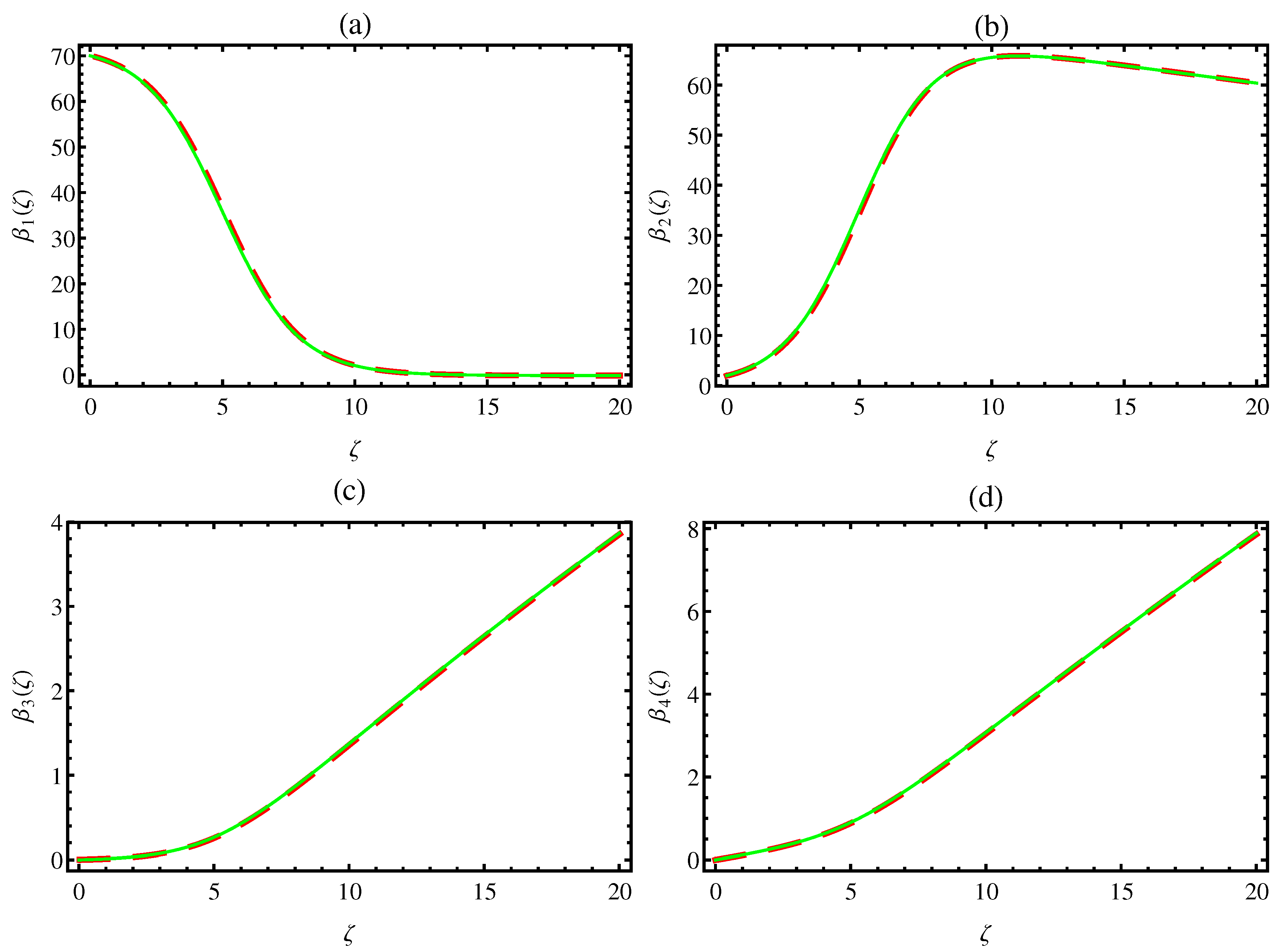
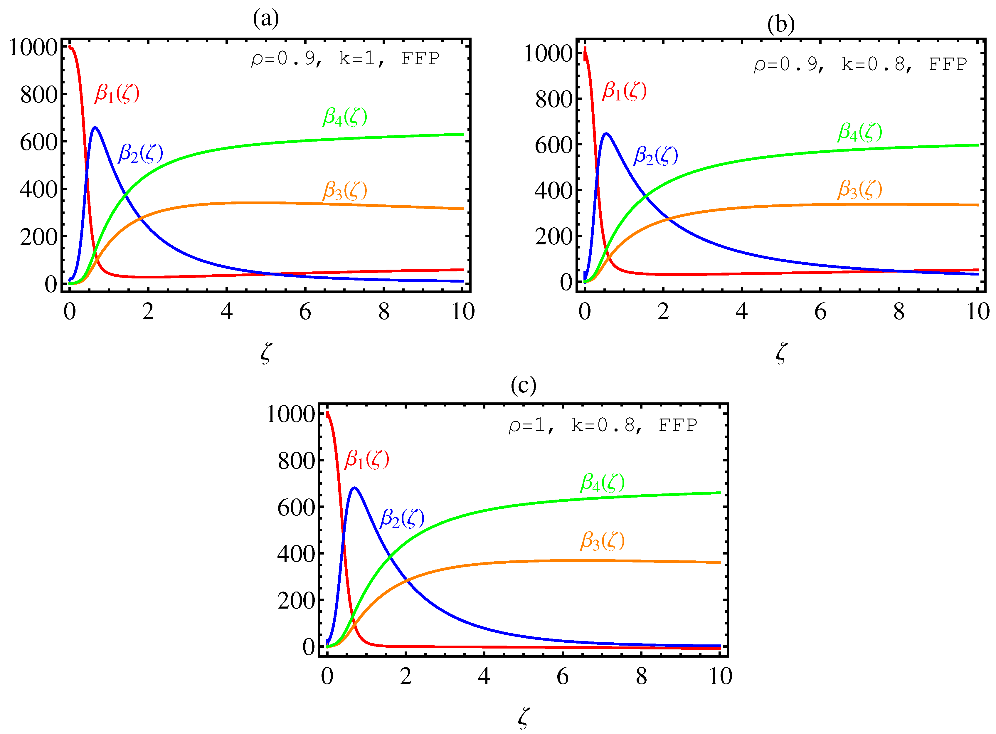
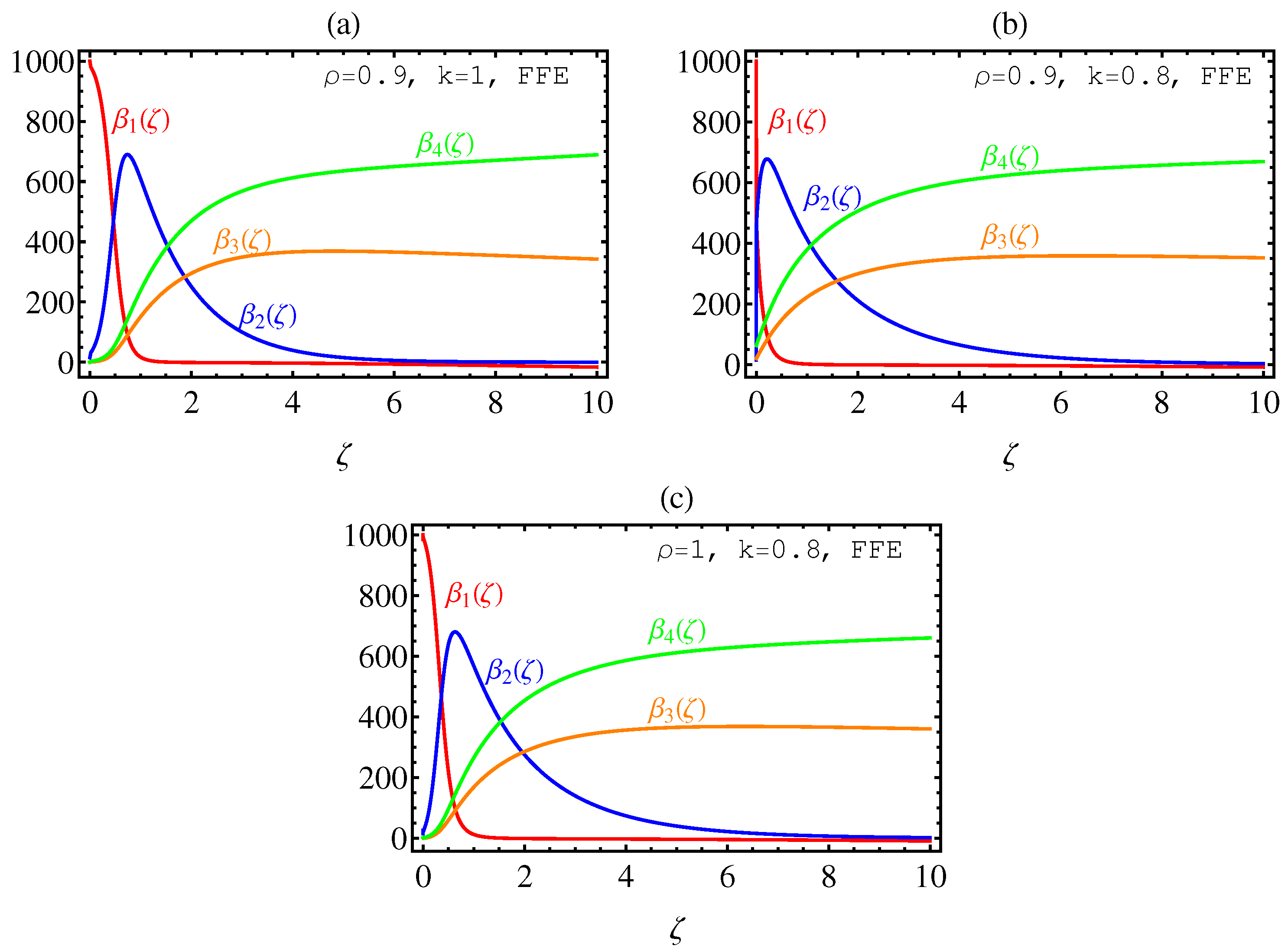
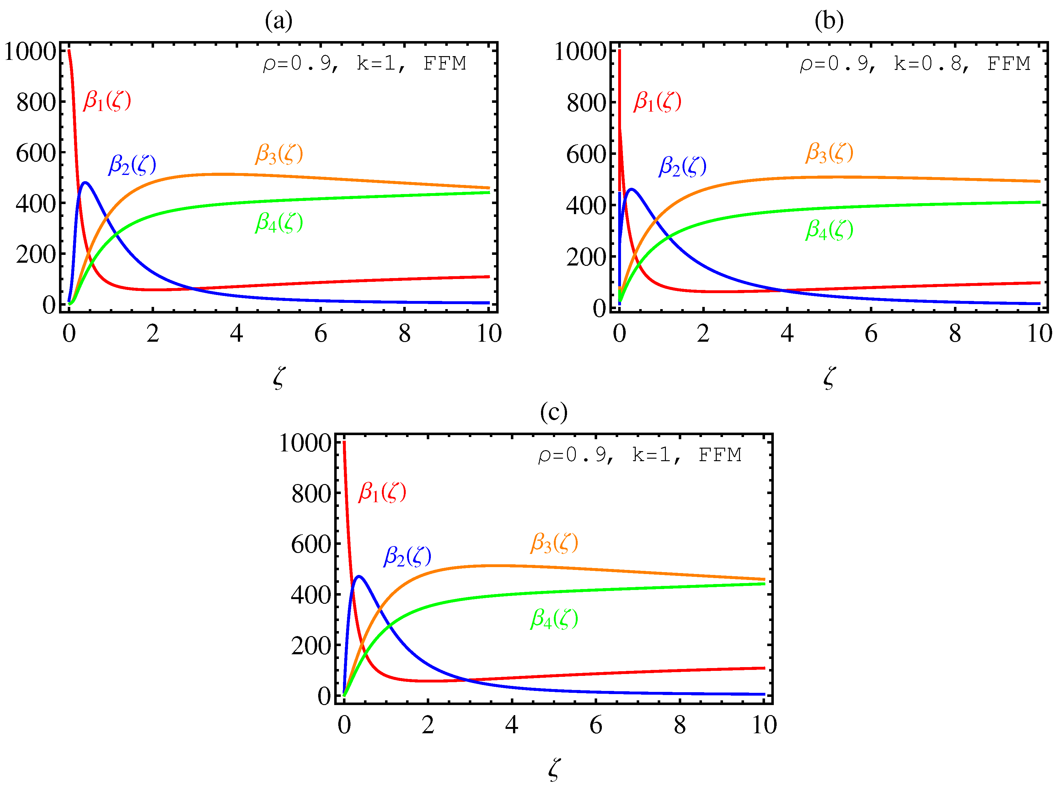
We first validate by means of our results in the case of the classical Ebola viruses in the case of the power kernel with a known numerical method such as the finite-difference method. We show satisfaction with the numerical solutions in the case of the power law kernel in sense of the Liouville-Caputo fractal-fractional derivative giving due credit also to Liouville who, in fact, considered such fractional derivatives many decades earlier in 1832. This is because all of the numerical solutions based on the three proposed kernels are close to each other at $\rho =k=1$. Figure 1a–d exhibit the comparison of the numerical solutions (20) found here and the numerical solutions based on the finite-difference method with $\rho =1$ and $k=1$. The parameters used here are $\lambda =0.01,s=0.002,\delta =0.006,\alpha =0.004,\beta =0.01,N=10,h=0.02$ and the initial conditions are ${\beta }_1\left(0\right)=70,{\beta }_2\left(0\right)=2,{\beta }_3\left(0\right)=0$ and ${\beta }_4\left(0\right)=0.$ From Figure 1a–d, we observe an excellent agreement, and the agreement is increasing as we increase the value of h. Figure 2, Figure 3 and Figure 4 show the behavior of the numerical solutions based upon on the constructions (20), (33) and (43), respectively. Numerical solutions are drawn for $\rho =0.9,k=1$, $\rho =0.9,k=0.8$, and $\rho =1,k=0.8$ in those sub-figures a to c, respectively. In these figures, we set the parameters as $\lambda =0.01,s=0.02,\delta =0.6,\alpha =0.4,\beta =0.01,N=1000,h=0.02$ and the initial conditions are given as follows:

$${\beta }_1\left(0\right)=1000,{\beta }_2\left(0\right)=15,{\beta }_3\left(0\right)=0\mathrm{and}{\beta }_4\left(0\right)=0.$$

In Figure 5, the numerical solutions (20), (33) and (43) are combined for $\rho =0.9,k=0.8,\lambda =0.01,s=0.02,\delta =0.6,\alpha =0.4,\beta =0.01,N=1000,h=0.0025$ and the following initial conditions:

$${\beta }_1\left(0\right)=1000,{\beta }_2\left(0\right)=15,{\beta }_3\left(0\right)=0\mathrm{and}{\beta }_4\left(0\right)=0.$$

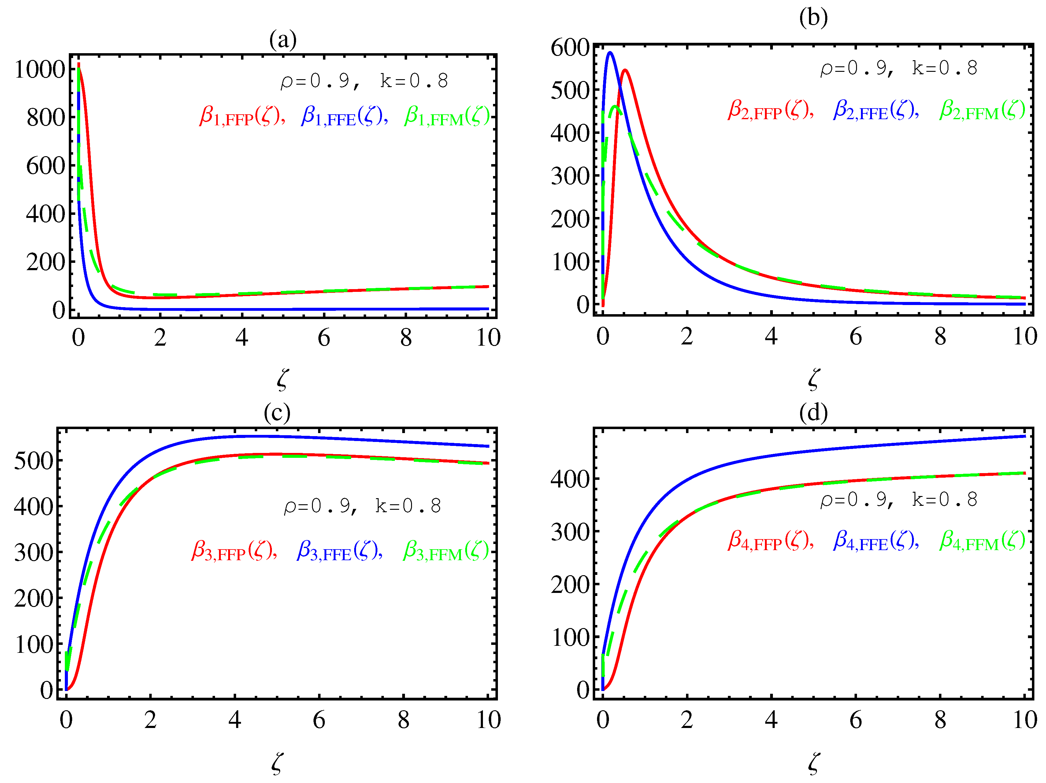
In fact, Figure 5 summarizes the behavior of numerical solutions (20), (33) and (43). The purpose of Figure 5 is not the numerical comparison between the three solutions, as each solution is based on an operator with a different kernel. Nevertheless, we find that the numerical solution (20) is much closer to the numerical solution (43) compared to the numerical solution (33).

6. Conclusions

In this paper, numerical solutions of three new models of the fractal-fractional Ebola virus have been studied. We have introduced the fractal-fractional Ebola virus in three instances of fractional derivatives based on the power law, the exponential law and the Mittag-Leffler kernels in the Liouville-Caputo concept which, in fact, was considered by Liouville many decades earlier in 1832. We have constructed three schemes for these three kernels. We have compared the numerical results used these schemes with those derived by using the finite-difference method in the case of integer order and and we have found an excellent agreement. Finally, the effects of the various values of the fractal and fractional order have been investigated and graphically illustrated in different figures.

The method presented in this paper is accurate and effective, and it can be used to find and study numerical solutions for many models related to the real-world situations. This method can be developed easily and, if we replace the Lagrange functions with other known functions, it will give rise to another field in the vast areas of numerical analysis. One of the advantages of this method is its ease of programming and obtaining realistic results.

In all of our calculations, we have used the Mathematica Program Package.

References

- Rachah, A.; Torres, D.F.M. Mathematical modelling, simulation, and optimal control of the 2014 Ebola outbreak in West Africa. Discret. Dyn. Nat. Soc. 2015, 3, 1–10. [Google Scholar] [CrossRef] [Green Version]
- Area, I.; Ndairou, F.; Nieto, J.J.; Silva, C.J. Ebola model and optimal control with vaccination constraints. J. Ind. Manag. Optim. 2018, 14, 427–446. [Google Scholar] [CrossRef] [Green Version]
- Mazandu, G.K.; Nembaware, V.; Thomford, N.E.; Bope, C.; Ly, O.; Chimusa, E.; Wonkam, A. A potential roadmap to overcome the current eastern DRC Ebola virus disease outbreak: From a computational perspective. Sci. Afr. 2020, 7, e00282. [Google Scholar] [CrossRef]
- Abdo, M.S.; Shah, K.; Wahash, H.A.; Panchal, S.K. On a comprehensive model of the novel Coronavirus (COVID-19) under Mittag-Leffler derivative. Chaos Solitons Fractals 2020, 135, 109867. [Google Scholar] [CrossRef] [PubMed]
- Ndairou, F.; Area, I.; Nieto, J.J.; Torres, D.F.M. Mathematical modeling of COVID-19 transmission dynamics with a case study of Wuhan. Chaos Solitons Fractals 2020, 135, 109846. [Google Scholar] [CrossRef] [PubMed]
- Postnikov, E.B. Estimation of COVID-19 dynamics “on a back-of-envelope”: Does the simplest SIR model provide quantitative parameters and predictions? Chaos Solitons Fractals 2020, 135, 109841. [Google Scholar] [CrossRef] [PubMed]
- Baseler, L.; Chertow, D.S.; Johnson, K.M.; Feldmann, H.; Morens, D.M. The pathogenesis of Ebola virus disease. Annu. Rev. Pathol. Mech. Dis. 2017, 12, 387–418. [Google Scholar] [CrossRef] [PubMed]
- Srivastava, H.M.; Dubey, R.S.; Jain, M. A study of the fractional-order mathematical model of diabetes and its resulting complications. Math. Methods Appl. Sci. 2019, 42, 4570–4583. [Google Scholar] [CrossRef]
- Ghanbari, B.; Günerhan, H.; Srivastava, H.M. An application of the Atangana-Baleanu fractional derivative in mathematical biology: A three-species predator-prey model. Chaos Solitons Fractals 2020, 138, 1–15. [Google Scholar] [CrossRef]
- Srivastava, H.M.; Günerhan, H. Analytical and approximate solutions of fractional-order susceptible-infected-recovered epidemic model of childhood disease. Math. Methods Appl. Sci. 2019, 42, 935–941. [Google Scholar] [CrossRef]
- Srivastava, H.M.; Shah, F.A.; Irfan, M. Generalized wavelet quasilinearization method for solving population growth model of fractional order. Math. Methods Appl. Sci. 2020, 43, 8753–8762. [Google Scholar] [CrossRef]
- Liao, S.-J. On the homotopy analysis method for nonlinear problems. Appl. Math. Comput. 2004, 147, 499–513. [Google Scholar] [CrossRef]
- Saad, K.M.; Al-Shareef, E.H.F.; Mohamed, M.S.; Yang, X.-J. Optimal q-homotopy analysis method for time-space fractional gas dynamics equation. Eur. Phys. J. Plus 2017, 132, 23. [Google Scholar] [CrossRef]
- Saad, K.M. A reliable analytical algorithm for spacetime fractional cubic isothermal autocatalytic chemical system. Pramana 2018, 91, 51. [Google Scholar] [CrossRef]
- Saad, K.M.; Al-Shareef, E.H.F.; Alomari, A.K.; Baleanu, D.; Gómez-Aguilar, J.F. On exact solutions for time-fractional Korteweg-de Vries and Korteweg-de Vries-Burgers equations using homotopy analysis transform method. Chinese J. Phys. 2020, 63, 149–162. [Google Scholar] [CrossRef]
- He, J.-H. Variational iteration method-a kind of nonlinear analytical technique: Some examples. Int. J. Nonlinear Mech. 1999, 34, 708–799. [Google Scholar] [CrossRef]
- Saad, K.M. and Al-Sharif, E.H. Analytical study for time and time-space fractional Burgers equation. Adv. Differ. Equa. 2017, 2017, 300. [Google Scholar] [CrossRef] [Green Version]
- Shi, X.-C.; Huang, L.-L.; Zeng, Y. Fast Adomian decomposition method for the Cauchy problem of the time-fractional reaction diffusion equation. Adv. Mech. Engrg. 2016, 8, 1–5. [Google Scholar] [CrossRef]
- Srivastava, H.M.; Saad, K.M.; Al-Sharif, E.H.F. A new analysis of the time-fractional and space-time fractional-order Nagumo equation. J. Inform. Math. Sci. 2018, 10, 545–561. [Google Scholar]
- Bueno-Orovio, A.; Kay, D.; Burrage, K. Fourier spectral methods for fractional-in-space reaction-diffusion equations. BIT Numer. Math. 2014, 54, 937–954. [Google Scholar] [CrossRef]
- Takeuchi, Y.; Yoshimoto, Y.; Suda, R. Second order accuracy finite difference methods for space-fractional partial di?erential equations. J. Comput. Appl. Math. 2017, 320, 101–119. [Google Scholar] [CrossRef]
- Çeneciz, Y.; Keskin, Y.; Kurnaz, A. The solution of the Bagley-Torvik equation with the generalized Taylor collocation method. J. Franklin Inst. 2010, 347, 452–466. [Google Scholar] [CrossRef]
- Khader, M.M.; Saad, K.M. A numerical approach for solving the fractional Fisher equation using Chebyshev spectral collocation method. Chaos Solitons Fractals 2018, 110, 169–177. [Google Scholar] [CrossRef]
- Saad, K.M. New fractional derivative with non-singular kernel for deriving Legendre spectral collocation method. Alex. Eng. J. 2020, 59, 1909–1917. [Google Scholar] [CrossRef]
- Kilbas, A.A.; Srivastava, H.M.; Trujillo, J.J. Theory and Applications of Fractional Differential Equations; North-Holland Mathematical Studies; Elsevier (North-Holland) Science Publishers: Amsterdam, The Netherlands; London, UK; New York, NY, USA, 2006. [Google Scholar]
- Podlubny, I. Fractional Differential Equations: An Introduction to Fractional Derivatives, Fractional Differential Equations, to Methods of Their Solution and Some of Their Applications, Mathematics in Science and Engineering; Academic Press: New York, NY, USA; London, UK; Sydney, Australia; Tokyo, Japan; Toronto, ON, Canada, 1999. [Google Scholar]
- Srivastava, H.M. Fractional-order derivatives and integrals: Introductory overview and recent developments. Kyungpook Math. J. 2020, 60, 73–116. [Google Scholar]
- Srivastava, H.M. Operators of basic (or q-) calculus and fractional q-calculus and their applications in geometric function theory of complex analysis. Iran. J. Sci. Technol. Trans. A: Sci. 2020, 44, 327–344. [Google Scholar] [CrossRef]
- Srivastava, H.M.; Saad, K.M.; Khader, M.M. An efficient spectral collocation method for the dynamic simulation of the fractional epidemiological model of the Ebola virus. Chaos Solitons Fractals 2020, 140, 110174. [Google Scholar] [CrossRef]
- Srivastava, H.M.; Saad, K.M.; Gómez-Aguilar, J.F.; Almadiy, A.A. Some new mathematical models of the fractional-order system of human immune against IAV infection. Math. Biosci. Eng. 2020, 17, 4942–4969. [Google Scholar] [CrossRef]
- Singh, H.; Srivastava, H.M. Numerical Simulation for Fractional-Order Bloch Equation Arising in Nuclear Magnetic Resonance by Using the Jacobi Polynomials. Appl. Sci. 2020, 10, 2850. [Google Scholar] [CrossRef] [Green Version]
- Caputo, M. Linear models of dissipation whose Q is almost frequency independent. II Geophys. J. R. Astron. Soc. 1967, 13, 529–539. [Google Scholar] [CrossRef]
- Caputo, M.; Fabrizio, M. A new defnition of fractional derivative without singular kernel. Progr. Fract. Differ. Appl. 2015, 1, 73–85. [Google Scholar]
- Atangana, A. Fractal-fractional differentiation and integration: Connecting fractal calculus and fractional calculus to predict complex system. Chaos Solitons Fractals 2017, 102, 396–406. [Google Scholar] [CrossRef]
- Li, Z.-F.; Liu, Z.-N.; Khan, M.A. Fractional investigation of bank data with fractal-fractional Caputo derivative. Chaos Solitons Fractals 2020, 131, 109528. [Google Scholar] [CrossRef]
- Gómez-Aguilar, J.F.; Atangana, A. New chaotic attractors: Application of fractal-fractional differentiation and integration. Math. Methods Appl. Sci. 2020. [Google Scholar] [CrossRef]
- Atangana, A.; Khan, M.A. Fatmawati, Modeling and analysis of competition model of bank data with fractal fractional Caputo-Fabrizio operator. Alex. Engrg. J. 2020, 59, 1985–1998. [Google Scholar] [CrossRef]
- Wang, W.-T.; Khan, M.A. Analysis and numerical simulation of fractional model of bank data with fractal-fractional Atangana-Baleanu derivative. J. Comput. Appl. Math. 2020, 369, 112646. [Google Scholar] [CrossRef]
- Srivastava, H.M.; Saad, K.M. New approximate solution of the time-fractional Nagumo equation involving fractional integrals without singular kernel. Appl. Math. Inform. Sci. 2020, 14, 1–8. [Google Scholar]
- Area, I.; Batarfi, H.; Losada, J.; Nieto, J.J.; Shammakh, W.; Torres-Iglesias, A. On a fractional order Ebola epidemic model. Adv. Differ. Equa. 2015, 2015, 1–8. [Google Scholar] [CrossRef] [Green Version]
- Bonyah, E.; Badu, K.; Asiedu-Addo, S.K. Optimal control application to an Ebola model. Asian Pac. J. Trop. Biomed. 2016, 6, 283–289. [Google Scholar] [CrossRef] [Green Version]
- Koca, I. Modelling the spread of Ebola virus with Atangana-Baleanu fractional operators. Eur. Phys. J. Plus 2018, 133, 100. [Google Scholar] [CrossRef]
- Rachah, A.; Torres, D.F.M. Predicting and controlling the Ebola infection. Math. Methods Appl. Sci. 2017, 40, 6155–6164. [Google Scholar] [CrossRef] [Green Version]
- Saad, K.M.; Gómez-Aguilar, J.F.; Almadiy, A.A. A fractional numerical study on a chronic hepatitis C virus infection model with immune response. Chaos Solitons Fractals 2020, 139, 110062. [Google Scholar] [CrossRef]
- Amundsen, S.B. Historical analysis of the Ebola virus: Prospective implications for primary care nursing today. Clin. Excell. Nurse Pract. 1998, 2, 343–351. [Google Scholar] [PubMed]
Figure 1.
Comparison between the numerical solutions (20) and numerical based on finite-difference methods for (a) (b) (c) and (d) , respectively, with and the following initial conditions: (Green solid color: Numerical solutions based on finite-difference methods; Red dashed color: Numerical solutions (20)).
Figure 2.
Graph of the numerical solutions based on FFP for (a) (b) and (c) , respectively, with and and the following initial conditions:
Figure 3.
Graph of the numerical solutions based on FFE for (a) , (b) and (c) , respectively, with and the following initial conditions:
Figure 4.
Graph of the numerical solutions based on FFM for (a) , (b) and (c) , respectively, with and the following initial conditions:
Figure 5.
Graph of the combined numerical solutions based on FFP, FFE and FFM for (a) (b) (c) and (d) , respectively, with and the following initial conditions: (Red solid color: Numerical solutions (20); Blue solid color: Numerical solutions (33); Green dashed color: Numerical solutions (43)).