A Collocation Method Based on Discrete Spline Quasi-Interpolatory Operators for the Solution of Time Fractional Differential Equations

Abstract

In many applications, real phenomena are modeled by differential problems having a time fractional derivative that depends on the history of the unknown function. For the numerical solution of time fractional differential equations, we propose a new method that combines spline quasi-interpolatory operators and collocation methods. We show that the method is convergent and reproduces polynomials of suitable degree. The numerical tests demonstrate the validity and applicability of the proposed method when used to solve linear time fractional differential equations.

1. Introduction

Fractional calculus refers to the calculus of integrals and derivatives of any real positive order [1,2,3]. During the last few years, it became very popular due to its applications in various fields of science and engineering. In fact, in many applications, real phenomena can be modeled by differential equations having a fractional derivative both in time and space. This allows one to take into account in a clear way the history and nonlocal behavior of the physical quantities under study. Through fractional calculus, we can study, for example, the viscoelasticity properties of special materials, anomalous diffusion in human tissues, water flow in deep ground, the prediction of earthquakes, and fractal problems [4,5,6,7].

There are several definitions of the fractional derivative that become equivalent under particular assumptions [1,3]. The first definition of a fractional derivative suitable for general functions appeared in the first half of the 19th Century and is now known as the Riemann–Liouville derivative:

$${{}_{RL}D}_t^{\gamma }y\left(t\right):=\frac{1}{\Gamma (m-\gamma )}\frac{d^m}{d{t}^m}{\int }_0^t\frac{y\left(\tau \right)}{{(t-\tau )}^{\gamma -m+1}}d\tau ,m-1<\gamma <m,m\in {\mathbb{N}}_{+},t>0,$$

(1)

where:

$$\Gamma \left(\alpha \right):={\int }_0^{\infty }{\tau }^{\alpha -1}{\mathrm{e}}^{-\tau }d\tau$$

is the Euler gamma function and ${\mathbb{N}}_{+}$ denotes the set of positive natural numbers.

Using the Riemann–Liouville definition, the usual differentiation operator in the Fourier domain can be easily extended to the fractional case, i.e.,

$$\mathcal{F}\left({{}_{RL}D}_t^{\gamma }y\left(t\right)\right)={\left(i\omega \right)}^{\gamma }\mathcal{F}\left(y\left(t\right)\right),\gamma \in {\mathbb{R}}_{+},$$

(2)

where $\mathcal{F}(·)$ denotes the Fourier transform operator. Moreover, the Riemann–Liouville derivative coincides with the Grunwald–Letnikov derivative

$${{}_{GL}D}_t^{\gamma }y\left(t\right)=\underset{\delta \to 0}{lim}\frac{1}{{\delta }^n}\sum _{k=0}^{\frac{t}{\delta }}{(-1)}^k\left(\genfrac{}{}{0pt}{}{\gamma }{k}\right)y(t-\delta k),$$

(3)

where:

$$\left(\genfrac{}{}{0pt}{}{\gamma }{k}\right):=\frac{\Gamma (\gamma +1)}{k!\Gamma (\gamma -k+1)},k\in \mathbb{N},\gamma \ge 0,$$

(4)

are the generalized binomial coefficients [1]. It is worth noticing that the sequence $\left\{\left(\genfrac{}{}{0pt}{}{\gamma }{k}\right)\right\}$ is compactly supported when $\gamma \in \mathbb{N}$, while for $\gamma \notin \mathbb{N}$, the sequence $\left\{\left(\genfrac{}{}{0pt}{}{\gamma }{k}\right)\right\}$ is no longer compactly supported, but its coefficients decay toward infinity as:

$$\left(\genfrac{}{}{0pt}{}{\gamma }{k}\right)\to k^{-\gamma -1}\mathrm{for}k\to \infty .$$

The Grunwald–Letnikov definition (3) is easier to use when addressing the numerical solution of fractional differential equations by finite difference methods [8].

The Riemann–Liouville derivative is not suitable to be used in real-world models for two main reasons: the Riemann–Liouville derivative of constant functions is not zero, and the initial conditions for initial value fractional differential problems are not easy to enforce. To overcome these problems, in 1967, Caputo [9] introduced a new definition of the fractional derivative, now named the Caputo derivative:

$${}_C{D}_t^{\gamma }y\left(t\right):=\frac{1}{\Gamma (m-\gamma )}{\int }_0^t\frac{y^{\left(m\right)}\left(\tau \right)}{{(t-\tau )}^{\gamma -m+1}}d\tau ,m-1<\gamma <m,m\in {\mathbb{N}}_{+},t>0.$$

(5)

The Riemann–Liouville derivative and the Caputo derivative are related to each other by:

$${}_C{D}_t^{\gamma }y\left(t\right)={{}_{RL}D}^{\gamma }\left(y\left(t\right)-\sum _{\ell =0}^{m-1}\frac{t^{\ell }}{\ell !}{y}^{(\ell )}\left(0^{+}\right)\right)$$

(6)

so that they coincide when the function $y\left(t\right)$ satisfies homogeneous initial conditions [1].

Even if the Caputo derivative requires higher smoothness of the function $y\left(t\right)$, it is more suitable to describe real phenomena since it shares some of the main properties with the ordinary derivative. In particular, the Caputo derivative of constant functions is zero, and the initial and boundary conditions are easy to implement. For this reason, in this paper, we consider an initial value differential problem having the Caputo derivative in time. For a discussion on other types of fractional derivatives, see [10].

In the literature, several numerical methods have been proposed to solve fractional differential equations [8,11,12]. Finite difference methods are very popular since they are easy to implement, but they require high order difference formulas to achieve high accuracy at the price of a high computational cost [13,14]. Spectral methods are more efficient since the solution to the differential problem is approximated by an expansion in a global polynomial basis, whose fractional derivative can be evaluated explicitly. However, the coefficients of the expansion are obtained by solving a dense linear system so that its numerical solution could have a high computational cost [11,14]. For this reason, expansions in local bases with small support are preferable. For instance, polynomial B-splines [15] are piecewise polynomials with small support that can be used to construct a basis for the spline space. In fact, spline functions are piecewise polynomials of a given degree and prescribed smoothness that can be constructed as linear combinations of B-splines. The freedom to choose the degree of the polynomial pieces and the overall smoothness of the spline give a great flexibility that can be used to adapt the spline to the function to be approximated.

As in the case of spectral methods, the expansion coefficients of the B-spline representation can be obtained using collocation methods with the advantage that the collocation matrix is triangular and the off-diagonal entries decay fast. In the case of cardinal B-splines, i.e., B-splines with uniform knots, their fractional derivative can be evaluated explicitly by the backward finite difference operator [16]. This approach was introduced by two of the authors in [17] (see also [18]), where a spline collocation method based on B-spline bases was used to solve a time fractional diffusion equation. The method proved to be particularly effective also in the case of nonlinear fractional differential equations [19]. A different approach was considered in [20,21], where the fractional differential equation under study was reformulated as an integral equation and solved by approximating its solution by a spline function represented by a Lagrange polynomial basis. More recently, a similar approach was used in [22] to solve multi-term fractional differential equations. For a comprehensive treatment of this topic, see [23].

In this paper, we propose a new method based on refinable spline quasi-interpolatory operators. Quasi-interpolatory operators have greater flexibility with respect to interpolation, since they are only required to reproduce polynomials up to a given degree rather than interpolate a function at given points. For this reason, they can be constructed to satisfy some special properties, such as shape preserving properties or prescribed approximation order. In more detail, we consider an initial value problem having the fractional derivative in time and approximate its solution by a family of discrete quasi-interpolatory operators [24,25,26]. Then, the unknown coefficients of the approximating function are determined by the collocation method introduced in [18]. The method presented here is a generalization of the collocation method introduced in [18,27]. The main novelty is the use of spline quasi-interpolatory operators as approximating functions so that the unknown coefficients are suitable functionals of the solution to the differential problem. Different choices of the functionals allow us to increase the polynomial reproducibility of the approximating function with the advantage of achieving higher accuracy. To our knowledge, this is the first time that quasi-interpolatory operators have been used to numerically solve differential equations having a fractional derivative.

Since the quasi-interpolatory operators we consider are spline functions, i.e., piecewise polynomials of integer degree, their fractional derivatives are fractional splines, i.e., piecewise polynomials of non-integer degree [16]. Thus, the fractional derivatives needed to evaluate the numerical solution by the collocation method can be computed efficiently by an explicit differentiation rule [28]. The numerical results show that the method is easy to implement and efficient so that it can be used to solve other kinds of fractional differential problems, such as boundary value problems and nonlinear problems.

The paper is organized as follows. Some preliminaries, needed to develop the numerical method, are given in Section 2. In particular, in Section 2.1, the fractional differential equation we are interested in is introduced, as well as its analytical solution expressed in terms of the Mittag–Leffler function. In Section 2.2, the spline space we use as the approximating space is described. In Section 2.3, the family of discrete spline quasi-interpolatory operators we use as approximating functions is defined, and its main properties are analyzed. The new method we propose is introduced in Section 3 where the explicit expression of the fractional derivative of the B-spline basis is also given (cf. Section 3.1). Finally, in Section 4, some numerical tests are performed. Section 5 is devoted to the discussion of our results, while in Section 6, some conclusions are offered.

2. Materials and Methods

2.1. Linear Fractional Differential Problems

Let us consider the following initial value problem:

$$\left\{\begin{array}{c}{{}_{C}D}_t^{\gamma }y\left(t\right)+by\left(t\right)=f\left(t\right),t>0,0<\gamma <1,\hfill \\ \\ y\left(0\right)=y_0,\hfill \end{array}\right.$$

(7)

where $b\in \mathbb{R}$ is a given parameter and $f\left(t\right)\in C[0,+\infty )$ is the inhomogeneous term. The well-posedness, existence, and uniqueness of the solution to the fractional differential problem (7) were analyzed in [3] (§6). In particular, the continuity of f guarantees that there exists a unique solution $y\in C[0,+\infty )$ that depends on a continuous way from the given data.

Using the Mittag–Leffler function [29]:

$$E_{\gamma ,\beta }\left(z\right)=\sum _{k=0}^{\infty }\frac{z^k}{\Gamma (\gamma k+\beta )},\gamma ,\beta \ge 0,z\in \mathbb{C},$$

the solution can be expressed in closed form as [3]:

$$y\left(t\right)=y_0{E}_{\gamma ,1}(-b{t}^{\gamma })+{\int }_0^{t}f(t-\tau ){\tau }^{\gamma -1}{E}_{\gamma ,\gamma }(-b{\tau }^{\gamma })d\tau .$$

(8)

Our main purpose is to solve the differential problem (7) by a collocation method based on spline quasi-interpolatory operators. Even if the fractional differential problem here considered can be solved analytically, nevertheless its solution is a good test for analyzing the approximation properties of the proposed method and studying its convergence.

2.2. B-Spline Spaces

The cardinal B-spline $B_n\left(t\right)$ is a piecewise polynomial of degree n having breakpoints on the integers. It can be defined through the backward finite difference operator, defined as:

$${\nabla }^{n}f\left(t\right):=\sum _{k=0}^n\left(\genfrac{}{}{0pt}{}{n}{k}\right){(-1)}^{k}f(t-k),$$

where f is a continuous function, applied to the truncated power function:

$$T_n\left(t\right):={\left(max(0,t)\right)}^n,n\in \mathbb{N},$$

i.e.,

$$B_n\left(t\right):=\frac{1}{n!}{\nabla }^{n+1}{T}_n\left(t\right),n\in \mathbb{N}.$$

(9)

The B-spline $B_n\left(t\right)$ is compactly supported on $I_n:=[0,n+1]$, positive in $(0,n+1)$, and belongs to $C^{n-1}\left(\mathbb{R}\right)$. For further details on spline functions, see [15,30].

The system of the integer translates $S_n=\left\{B_n(t-k),k\in \mathbb{Z}\right\}$, forming a basis for the space of spline functions of degree n. It reproduces polynomials up to degree n, i.e.,

$$t^{r-1}=\sum _{k\in \mathbb{Z}}{\xi }_k^{\left(r\right)}{B}_n(t-k),t\in \mathbb{R},1\le r\le n+1,$$

(10)

with:

$${\xi }_k^{\left(r\right)}=\frac{sym{m}_{r-1}(k+1,\dots ,k+n)}{\left(\genfrac{}{}{0pt}{}{n}{r-1}\right)},k\in \mathbb{Z},$$

(11)

where $sym{m}_r(t_1,\dots ,t_p)$ denotes the symmetric function defined as:

$$sym{m}_r(t_1,\dots ,t_p)=\sum _{1\le k_1<k_2<\cdots <k_r\le p}{t}_{k_1}{t}_{k_2}\cdots t_{k_r}.$$

(cf. [15]). In particular, for $r=1$, it holds:

$$1=\sum _{k\in \mathbb{Z}}{B}_n(t-k),t\in \mathbb{R},n\in \mathbb{N},$$

(12)

i.e., the function system $S_n$ forms a partition of unity, while for $r=2$, we get:

$$t=\sum _{k\in \mathbb{Z}}\left(k+\frac{n+1}{2}\right)B_n(t-k),t\in \mathbb{R},n\in {\mathbb{N}}_{+}.$$

The cardinal B-spline $B_n\left(t\right)$ can be adapted to any set of equidistant breakpoints by dilation. In particular, choosing the dyadic nodes $\{2^{-j}k,k\in \mathbb{Z}\}$ as breakpoints, we can define the refined basis:

$$S_{nj}=\{B_{njk}\left(t\right),k\in \mathbb{Z}\},j\in \mathbb{Z},$$

(13)

where the basis functions:

$$B_{njk}\left(t\right)=B_n(2^{j}t-k),k\in \mathbb{Z},j\in \mathbb{Z},$$

(14)

are the dilates and translates of $B_n\left(t\right)$ having support on $[2^{-j}k,2^{-j}(k+n+1)]$. Analogous to (10), for any $j\in \mathbb{N}$, one has:

$$t^{r-1}=\sum _{k\in \mathbb{Z}}{\xi }_{jk}^{\left(r\right)}{B}_{njk}\left(t\right),t\in \mathbb{R},1\le r\le n+1,$$

(15)

where the coefficients $\left\{{\xi }_{jk}^{\left(r\right)}\right\}$ are given by:

$${\xi }_{jk}^{\left(r\right)}=\frac{sym{m}_{r-1}(2^{-j}(k+1),\dots ,2^{-j}(k+n))}{\left(\genfrac{}{}{0pt}{}{n}{r-1}\right)},k\in \mathbb{Z},j\in \mathbb{N}.$$

(16)

2.3. Refinable Spline Quasi-Interpolatory Operators

Our interest is in the numerical solution of the fractional differential problem (7) using as the approximating function a quasi-interpolatory refinable operator constructed using the refinable basis $S_{nj}$.

Let $\mathcal{F}$ be a linear space of real-valued functions, and let $\left\{{\lambda }_{ji}\right\}$ be a set of linear functionals ${\lambda }_{ji}:\mathcal{F}\to \mathbb{R}$. We assume that $\mathcal{F}$ contains the class ${\mathbb{P}}_r$ of polynomials of degree at most $r-1$ with $1\le r\le n+1$. Given a function $f\in \mathcal{F}$, a refinable quasi-interpolatory operator $Q_{nj}f$ is an approximation to f of the form:

$$Q_{nj}f\left(t\right)=\sum _{k\in \mathbb{Z}}\left({\lambda }_{jk}f\right)B_{njk}\left(t\right),t\in \mathbb{R},j\in \mathbb{Z},$$

(17)

such that $Q_{nj}f$ is exact on polynomials up to degree $r-1$, $1\le r\le n+1$. We notice that, since any $B_{njk}\left(t\right)$ has compact support, for any $t\in \mathbb{R}$, the sum in (17) is actually a finite sum.

It is easy to show that $Q_{nj}f$ reproduces polynomials up to degree $r-1$ if and only if:

$${\lambda }_{jk}{t}^{\ell -1}={\xi }_{jk}^{(\ell )},1\le \ell \le r,k\in \mathbb{Z},$$

(18)

where ${\xi }_{jk}^{(\ell )}$ are the coefficients defined in (16) (cf. [25]). Since we will use the operator (17) to approximate the solution to the differential problem (7) in a finite discretization interval $I=[0,T]$, $T\in {\mathbb{N}}_{+}$, in the following, we will consider the operator $Q_{nj}f$ restricted to the interval I, i.e.,

$$Q_{nj}f\left(t\right)=\sum _{k=-n}^{N_j}\left({\lambda }_{jk}f\right)B_{njk}\left(t\right),t\in I,j\ge j_0,$$

(19)

where $N_j=2^{j}T-1$ and $j_0\ge \lceil {log}_2((n+1)/T)\rceil$ is the starting refinement level.

To enforce (18), we express the functionals ${\lambda }_{jk}f$ as:

$${\lambda }_{jk}f=\sum _{i=1}^r{\alpha }_{jki}\left({\lambda }_{jki}f\right),1\le r\le n+1,-n\le k\le N_j,$$

(20)

where ${\alpha }_{jki}$ are real coefficients to be determined and ${\lambda }_{jki}f:\mathcal{F}\to \mathbb{R}$ are linear functionals such that:

$$\det {\left({\lambda }_{jki}{t}^{\ell -1}\right)}_{1\le \ell ,i\le r}\ne 0.$$

(21)

There are several kinds of spline quasi-interpolatory operators [15,24,26,31,32,33,34]. A possible choice is to express the linear functionals $\left\{{\lambda }_{jik}\right\}$ through divided difference operators. Let $\{{\tau }_{ji1},\dots ,{\tau }_{jik}\}$ be a set of k distinct points in $I\cap supp\left(B_{njk}\right)$. Then, we set:

$${\lambda }_{jki}f=[{\tau }_{jk1},\cdots ,{\tau }_{jki}]f,1\le i\le r,1\le r\le n+1,$$

(22)

i.e., the difference operator of order $i-1$. Therefore, we get the discrete quasi-interpolatory operator [24,26]:

$$d{Q}_{nj}f\left(t\right)=\sum _{k=-n}^{N_j}\sum _{i=1}^r{\alpha }_{jki}\left([{\tau }_{jk1},\cdots ,{\tau }_{jki}]f\right)B_{njk}\left(t\right).$$

(23)

Proposition 1.

The discrete quasi-interpolatory operator $d{Q}_{nj}f$ reproduces polynomials up to degree $r-1$ with $1\le r\le n+1$ if and only if:

$$\sum _{i=1}^r{\alpha }_{jki}\left([{\tau }_{jk1},\cdots ,{\tau }_{jki}]t^{\ell -1}\right)={\xi }_{jk}^{(\ell )},1\le \ell \le r,-n\le k\le N_j,$$

(24)

where ${\xi }_{jk}^{(\ell )}$, $1\le \ell \le n+1$ are given in (16).

Proof. 

The proof is similar to that in [35] (Corollary 1). For any k held fixed, (24) represents a linear system of r equations in the r unknowns $\left\{{\alpha }_{jki}\right\}$. Given the particular choice of the functionals $\left\{{\lambda }_{jki}\right\}$ in (22), one has $\det \left({\lambda }_{jki}{t}^{r-1}\right)\ne 0$, $1\le r\le n+1$, $-n\le k\le N_j$, so that the linear system has a unique solution.

Without loss of generality, we set $r=n+1$ in (24). Then, inserting (24) into (23), we get:

$$d{Q}_{nj}{t}^{\ell -1}=\sum _{k=-n}^{N_j}\sum _{i=1}^{n+1}{\alpha }_{jki}[{\tau }_{jk1}\cdots {\tau }_{jki}]t^{\ell -1}{B}_{njk}\left(t\right)=\sum _{i=-n}^{N_j}{\xi }_{jk}^{\left(l\right)}{B}_{njk}\left(t\right)=t^{\ell -1},1\le \ell \le r+1,$$

i.e., the operator $d{Q}_{nj}$ reproduces polynomials up to degree $r-1$. Oppositely, using (24) in (15), we get $d{Q}_{nj}$ applied to monomials, and the claim follows. □

The coefficient matrix of the linear system (24) is lower triangular so that its solution can be obtained by the forward technique [24], i.e.,

$${\alpha }_{jki}=\sum _{s=0}^{i-1}{\left(-1\right)}^s{\xi }_{jk}^{\left(i-s\right)}sym{m}_s({\tau }_{jk1},\cdots ,{\tau }_{jki-1}),1\le i\le r,-n\le k\le N_j.$$

(25)

In particular, from (25), it follows:

$${\alpha }_{jk1}=1,{\alpha }_{jk2}={\xi }_{jk}^{\left(2\right)}-{\tau }_{jk1},$$

so that for $r=1$, we get:

$$d{Q}_{nj}f\left(t\right)=\sum _{k=-n}^{N_j}f\left({\tau }_{jk1}\right)B_{njk}\left(t\right),$$

(26)

which is the operator reproducing just the constant function considered in [28], while for $r=2$, we get:

$$d{Q}_{nj}f\left(t\right)=\sum _{k=-n}^{N_j}\frac{f\left({\tau }_{jk2}\right)({\xi }_{jk}^{\left(2\right)}-{\tau }_{jk1})-f\left({\tau }_{jk1}\right)({\xi }_{jk}^{\left(2\right)}-{\tau }_{jk2})}{{\tau }_{jk2}-{\tau }_{jk1}}{B}_{njk}\left(t\right).$$

(27)

3. Numerical Method

For any fixed $j\ge j_0$, we approximate the solution to the fractional differential problem (7) by the discrete quasi-interpolatory operator (23), i.e.,

$$y\left(t\right)\approx y_{nj}\left(t\right)=\sum _{k=-n}^{N_j}\sum _{i=1}^r{\alpha }_{jki}\left([{\tau }_{jk1},\cdots ,{\tau }_{jki}]y\right)B_{njk}\left(t\right),$$

(28)

where $\left\{{\alpha }_{jki}\right\}$ are the coefficients defined in (25) and:

$$y_{jki}=[{\tau }_{jk1}\cdots {\tau }_{jki}]y,1\le i\le r,-n\le k\le N_j,j\ge j_0,$$

are the unknown coefficients whose expression depends on the polynomial reproducibility order r. In particular, for $r=1$:

$$y_{jki}=y\left({\tau }_{jk1}\right)$$

while for $r=2$:

$$y_{jki}=\frac{y\left({\tau }_{jk2}\right)({\xi }_{jk}^{\left(2\right)}-{\tau }_{jk1})-y\left({\tau }_{jk1}\right)({\xi }_{jk}^{\left(2\right)}-{\tau }_{jk2})}{{\tau }_{jk2}-{\tau }_{jk1}},$$

where ${\tau }_{jki}$, $-n\le k\le N_j$, $i=1,2$ are given distinct points in the interval $[2^{-j}k,2^{-j}(k+n+1)]\cap I$.

We determine the unknown coefficients by collocation. To this end, we choose a set of collocation points $\{t_p,0\le p\le N_P\}$ that belong to the discretization interval I and enforce the approximating function $y_{nj}\left(t\right)$ to solve the differential problem on these points, i.e.,

$$\left\{\begin{array}{cc}{{}_{C}D}_t^{\gamma }{y}_{nj}\left(t_p\right)+b{y}_{nj}\left(t_p\right)=f\left(t_p\right),\hfill & 1\le p\le N_s,\hfill \\ \\ y_{nj}\left(0\right)=y_0.\hfill \end{array}\right.$$

(29)

Substituting (28) in the previous equations and rearranging the sums, we get:

$$\left\{\begin{array}{cc}{\displaystyle \sum _{k=-n}^{N_j}{{}_{C}D}_t^{\gamma }{B}_{njk}\left(t_p\right)\sum _{i=1}^r{\alpha }_{jki}\left(y_{jki}\right)+b\sum _{k=-n}^{N_j}{B}_{njk}\left(t_p\right)\sum _{i=1}^r{\alpha }_{jki}\left(y_{jki}\right)=f\left(t_p\right),}\hfill & 1\le p\le N_s,\hfill \\ \\ {\displaystyle \sum _{k=-n}^{N_j}{B}_{njk}\left(0\right)\sum _{i=1}^r{\alpha }_{jki}\left(y_{jki}\right)=y_0.}\hfill \end{array}\right.$$

(30)

Equations (30) form a linear system that can be written in matrix form as:

$$\left\{\begin{array}{c}\left(D_{njs}+b{B}_{njs}\right)A_{jr}{C}_{jr}=F_s,\hfill \\ \\ V_{njs}{A}_{jr}{C}_{jr}=y_0.\hfill \end{array}\right.$$

(31)

where $C_{jr}={[y_{jki},1\le i\le r,-n\le k\le N_j]}^T$ is the unknown column vector,

$$A_{jr}=[diag\left(a_{j\ell }\right),1\le \ell \le r]\in {\mathbb{R}}^{(N_j+n+1)\times (N_j+n+1)r},a_{j\ell }=[{\alpha }_{jk\ell },-n\le k\le N_j],$$

is the matrix collecting the coefficients $\left\{{\alpha }_{jki}\right\}$, $V_{njs}=[B_{njk}\left(0\right),-n\le k\le N_j]$ is the row vector whose entries are the basis functions evaluated at the initial point $t=0$,

$$\begin{array}{c}{D}_{njs}=\left[{{}_{C}D}_t^{\gamma }{B}_{njk}\left(t_p\right),1\le p\le N_s,-n\le k\le N_j\right]\in {\mathbb{R}}^{N_s\times (N_j+n+1)},\hfill \\ \\ B_{njs}=\left[B_{njk}\left(t_p\right),1\le p\le N_s,-n\le k\le N_j\right]\in {\mathbb{R}}^{N_s\times (N_j+n+1)},\hfill \end{array}$$

are the collocation matrices of the refinable basis, and:

$$F_s={[f\left(t_p\right),1\le p\le N_s]}^T,$$

is the known term.

The linear system (31) has $N_s+1$ equations and $(N_j+n+1)r$ unknowns. To guarantee the existence of a unique solution, for any fixed n and r, the number of collocation points $N_s+1$ and the refinement level j have to be chosen so that number of unknowns is no greater than the number of equations (cf. [27,36]). In the case when $N_s+1>(N_j+n+1)r$, (31) results in an overdetermined linear system that can be solved by the least squares method. In this case, particular attention should be paid to fulfill the initial condition.

We notice that from the partition of unity property (12) and [18] (Th. 3.1), it follows that the collocation solution $y_{nj}\left(t\right)$ is stable, i.e.,

$$\parallel y_{nj}{\left(t\right)\parallel }_{\infty }\le \kappa {\parallel f\parallel }_{\infty },$$

where $\kappa$ is a constant independent of j.

Finally, the collocation method can be proven to be convergent (cf. [27,28]).

Theorem 1.

The collocation method is convergent, i.e.:

$$\underset{j\to \infty }{lim}{\parallel y\left(t\right)-y_{nj}\left(t\right)\parallel }_{\infty }=0,$$

with convergence order ν provided that $y\in C^{\nu }[0,T]$, i.e.,

$$\parallel y\left(t\right)-y_{nj}{\left(t\right)\parallel }_{\infty }=O\left(2^{-j\nu }\right).$$

Proof. 

Using Definition (5), it is easy to show that the fractional differential equation (7) is equivalent to the integral equation:

$$z\left(t\right)+\frac{b}{\Gamma \left(\gamma \right)}{\int }_0^t\frac{z\left(\tau \right)}{{(t-\tau )}^{1-\gamma }}d\tau =f\left(t\right),$$

where $z\left(t\right)={{}_{C}D}_t^{\gamma }y\left(t\right)$. The collocation method can be used also to approximate the solution to this integral equation, i.e.,

$$z_{nj}\left(t_p\right)+\frac{b}{\Gamma \left(\gamma \right)}{\int }_0^{t_p}\frac{z_{nj}\left(\tau \right)}{{(t_p-\tau )}^{1-\gamma }}d\tau =f\left(t_p\right),1\le p\le N_s,$$

where $z_{nj}\left(t\right)$ is the quasi-interpolatory operator (23). Thus, the equivalence implies that the approximation error $\parallel y\left(t\right)-y_{nj}{\left(t\right)\parallel }_{\infty }$ is the same as the approximation error $\parallel z\left(t\right)-z_{nj}{\left(t\right)\parallel }_{\infty }$ (cf. [36]). Since $z_{nj}$ is a spline operator, the convergence is guaranteed with approximation order $\nu$ when $y\in C^{\nu }[0,T]$ [30]. □

3.1. The Fractional Derivative of the Refinable B-Spline Basis

To numerically solve the linear system (31), we need to evaluate the Caputo derivative of the basis functions $B_{njk}$, $-n\le k\le N_j$. For $0\le k\le N_j$, the Caputo derivative of $B_{njk}\left(t\right)$ can be explicitly evaluated by [18,27]:

$${{}_{C}D}_t^{\gamma }{B}_{njk}\left(t\right)=2^{\gamma j}\frac{{\Delta }^{n+1}{T}_{n-\gamma }(2^{j}t-k)}{\Gamma (n-\gamma +1)},0<\gamma \le n.$$

(32)

For $-n\le k\le -1$, the functions $B_{njk}$ are left edge functions having support on $[0,2^{-j}(n+k+1)]$. When $0<\gamma <1$, their fractional derivative can be explicitly evaluated by [27]:

$${{}_{C}D}_t^{\gamma }{B}_{njk}\left(t\right)=2^{\gamma j}\frac{{\Delta }^{n+1}{T}_{n-\gamma }(2^{j}t-k)-L_{njk}\left(2^{j}t\right)}{\Gamma (n+1-\gamma )},n\ge 1,$$

(33)

where:

$$\begin{array}{ccc}{L}_{njk}\left(t\right)\hfill & =& {\displaystyle \sum _{i=0}^{-k-1}{(-1)}^i\left(\genfrac{}{}{0pt}{}{n+1}{i}\right)({(t-k-i)}^{n-\gamma }+}\hfill \\ \\ \hfill & & {\displaystyle t^{1-\gamma }\sum _{p=0}^{n-1}\frac{{(-1)}^{n-p}{(-k-i)}^{n-1-p}{(t-k-i)}^p}{(n-1-p)!}\prod _{s=1}^{n-1-p}(\gamma -s)),-n\le k\le -1.}\hfill \end{array}$$

(34)

We assume ${\prod }_{s=1}^p(\gamma -s)=1$ when $p<1$.

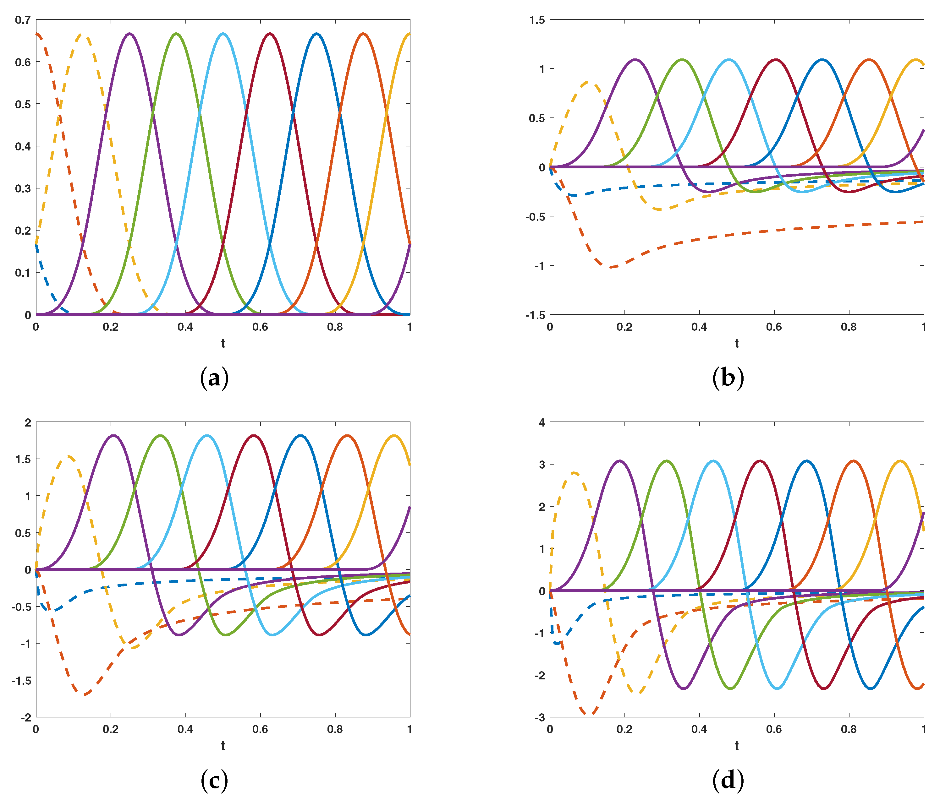
In Figure 1, the cubic basis $S_{3j}$ and its fractional derivatives at the refinement level $j=3$ are shown for some values of the fractional derivative $\gamma$.

4. Numerical Results

In this section, we show the numerical solutions we obtain by the collocation method introduced in the previous section.

For the sake of simplicity, in the tests, we chose as collocation points the dyadic points of the interval I, i.e.,

$$\left\{t_p=\frac{p}{2^s},0\le p\le N_s\right\},$$

(35)

where $N_s=2^{s}T$ and $s\ge 0$ is the collocation level. Moreover, we used as approximating spaces the refinable spaces generated by the cubic B-spline basis $S_{3j}$, and we set $s=j+1$ so that the time step is $\Delta t=2^{-j-1}$. We used as approximating functions the two discrete quasi-interpolatory operators $d{Q}_{3j}y$ obtained by setting $n=3$, $r=1$, and $r=2$ in (23), i.e., the operators given in (26) and (27), respectively. The points ${\tau }_{jk1}$ and ${\tau }_{jk2}$ are the endpoints of $supp{B}_{3jk}$, i.e.,

$${\tau }_{jk1}=min(0,2^{-j}k),{\tau }_{jk2}=max(2^{-j}(k+4),T),-3\le k\le N_j,j\ge j_0.$$

To analyze the performance of the collocation method, we evaluate the infinity norm of the approximation error $e_{3j}\left(t\right)=y\left(t\right)-y_{3j}\left(t\right)$, i.e.,

$$\parallel e_{3j}{\parallel }_{\infty }=\underset{\begin{array}{c}0\le p\le 3N_s\end{array}}{max}\left|e_{3j}\left(t_p\right)\right|,\left\{t_p=\frac{p}{3·2^s},0\le p\le 3N_s\right\},$$

and the numerical convergence order defined as:

$${\rho }_{3j}={log}_2\left(\frac{\parallel e_{3,j-1}{\parallel }_{\infty }}{\parallel e_{3j}{\parallel }_{\infty }}\right).$$

For the ease of notation, in the following, we will drop the subscript 3.

4.1. Example 1

In the first example, we set $b=0$, $f\left(t\right)=\frac{\Gamma (\mu +1)}{\Gamma (\mu +1-\gamma )}{t}^{\mu -\gamma }$ and $y\left(0\right)=0$ so that the initial value problem (7) becomes:

$$\left\{\begin{array}{c}{{}_{C}D}_t^{\gamma }y\left(t\right)=\frac{\Gamma (\mu +1)}{\Gamma (\mu +1-\gamma )}{t}^{\mu -\gamma },0<t\le 1,0<\gamma <1,\hfill \\ \\ y\left(0\right)=0.\hfill \end{array}\right.$$

In this case, the exact solution is $y\left(t\right)=t^{\mu }$. The discretization interval is $I=[0,1]$.

Since the proposed method reproduces polynomials up to degree three when using the cubic B-spline basis, to check the polynomial reproducibility, in the first test, we set $\mu =3$. Thus, the approximation is exact, and we expect the approximation error to be zero. Actually, the results listed in

Table 1. Example 1: The infinity norm of the error $\parallel e_j{\parallel }_{\infty }$ for $\mu =3$ and different values of the fractional derivative $\gamma$ and the refinement level j when using $d{Q}_{3j}y$ with $r=1$ and $r=2$ (cf. (26) and (27)). The number of collocation points is $N_s+1=2^j+1$.

		$\mathit{\gamma }=0.25$		$\mathit{\gamma }=0.5$		$\mathit{\gamma }=0.75$
$\mathit{j}$	${\mathit{N}}_{\mathit{s}}+\mathbf{1}$	$\mathit{r}=\mathbf{1}$	$\mathit{r}=\mathbf{2}$	$\mathit{r}=\mathbf{1}$	$\mathit{r}=\mathbf{2}$	$\mathit{r}=\mathbf{1}$	$\mathit{r}=\mathbf{2}$
3	17	3.33$\times {10}^{-16}$	4.44$\times {10}^{-16}$	4.44$\times {10}^{-16}$	2.10$\times {10}^{-16}$	7.77$\times {10}^{-16}$	1.26$\times {10}^{-15}$
4	33	1.33$\times {10}^{-15}$	1.89$\times {10}^{-15}$	6.88$\times {10}^{-15}$	2.00$\times {10}^{-15}$	2.22$\times {10}^{-15}$	1.78$\times {10}^{-15}$
5	65	7.80$\times {10}^{-14}$	3.84$\times {10}^{-14}$	4.71$\times {10}^{-14}$	1.78$\times {10}^{-14}$	1.95$\times {10}^{-14}$	1.84$\times {10}^{-14}$
6	129	7.17$\times {10}^{-13}$	1.06$\times {10}^{-12}$	1.71$\times {10}^{-13}$	3.04$\times {10}^{-13}$	1.14$\times {10}^{-13}$	2.95$\times {10}^{-13}$

show that the infinity norm of the error is in the order of machine precision for both quasi-interpolatory operators $d{Q}_{3j}y$ with $r=1$ and $r=2$.

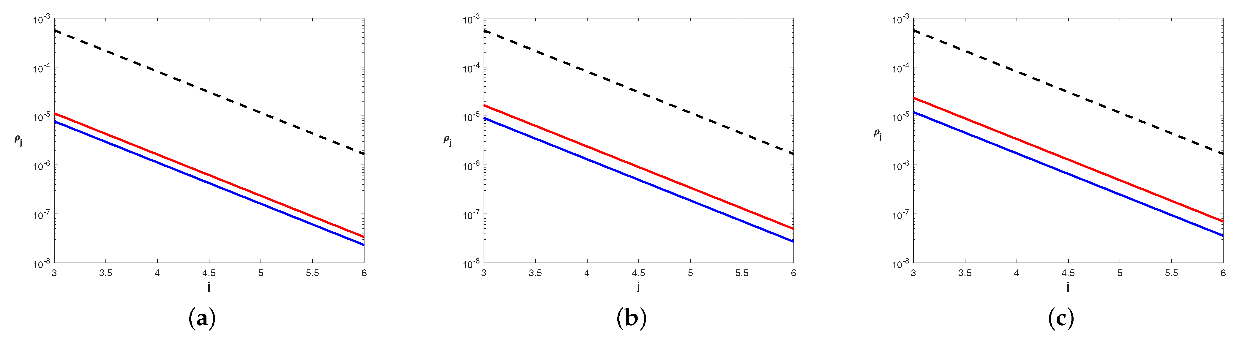
To check the convergence order, in the second test, we set $\mu =2.8$ so that the theoretical convergence order is precisely $\mu$. The numerical convergence order for different values of $\gamma$ is displayed in Figure 2 as a function of the refinement level j. For comparison, a line having the same slope as the theoretical convergence order is also displayed. The infinity norm of the approximation error and the numerical convergence order are listed in

Table 2. Example 1: The infinity norm of the error and the numerical convergence order for different values of the fractional derivative $\gamma$ and the refinement level j when using $d{Q}_{3j}y$ with $r=1$ (cf. (26)). The number of collocation points is $N_s+1=2^j+1$.

		$\mathit{\gamma }=0.25$		$\mathit{\gamma }=0.5$		$\mathit{\gamma }=0.75$
$\mathit{j}$	${\mathit{N}}_{\mathit{s}}+\mathbf{1}$	$\parallel {\mathit{e}}_{\mathit{j}}{\parallel }_{\infty }$	${\mathit{\rho }}_{\mathit{j}}$	$\parallel {\mathit{e}}_{\mathit{j}}{\parallel }_{\infty }$	${\mathit{\rho }}_{\mathit{j}}$	$\parallel {\mathit{e}}_{\mathit{j}}{\parallel }_{\infty }$	${\mathit{\rho }}_{\mathit{j}}$
3	17	1.13$\times {10}^{-5}$		1.65$\times {10}^{-5}$		2.35$\times {10}^{-5}$
4	33	1.63$\times {10}^{-6}$	2.800	2.38$\times {10}^{-6}$	2.800	3.37$\times {10}^{-6}$	2.800
5	65	2.34$\times {10}^{-7}$	2.800	3.41$\times {10}^{-7}$	2.800	4.84$\times {10}^{-7}$	2.800
6	129	3.35$\times {10}^{-8}$	2.800	4.90$\times {10}^{-8}$	2.800	6.96$\times {10}^{-8}$	2.800

and

Table 3. Example 1: The infinity norm of the error and the numerical convergence order for different values of the fractional derivative $\gamma$ and the refinement level j when using $d{Q}_{3j}y$ with $r=2$ (cf. (27)). The number of collocation points is $N_s+1=2^j+1$.

		$\mathit{\gamma }=0.25$		$\mathit{\gamma }=0.5$		$\mathit{\gamma }=0.75$
$\mathit{j}$	${\mathit{N}}_{\mathit{s}}+\mathbf{1}$	$\parallel {\mathit{e}}_{\mathit{j}}{\parallel }_{\infty }$	${\mathit{\rho }}_{\mathit{j}}$	$\parallel {\mathit{e}}_{\mathit{j}}{\parallel }_{\infty }$	${\mathit{\rho }}_{\mathit{j}}$	$\parallel {\mathit{e}}_{\mathit{j}}{\parallel }_{\infty }$	${\mathit{\rho }}_{\mathit{j}}$
3	17	7.77$\times {10}^{-6}$		9.07$\times {10}^{-6}$		1.20$\times {10}^{-5}$
4	33	1.12$\times {10}^{-6}$	2.800	1.30$\times {10}^{-6}$	2.800	1.72$\times {10}^{-6}$	2.800
5	65	1.60$\times {10}^{-7}$	2.800	1.87$\times {10}^{-7}$	2.800	2.47$\times {10}^{-7}$	2.800
6	129	2.30$\times {10}^{-8}$	2.800	2.69$\times {10}^{-8}$	2.800	3.55$\times {10}^{-8}$	2.800

. Table 2 refers to the quasi-interpolatory operators $d{Q}_{3j}y$ with $r=1$, while Table 3 refers to the case $r=2$.

4.2. Example 2

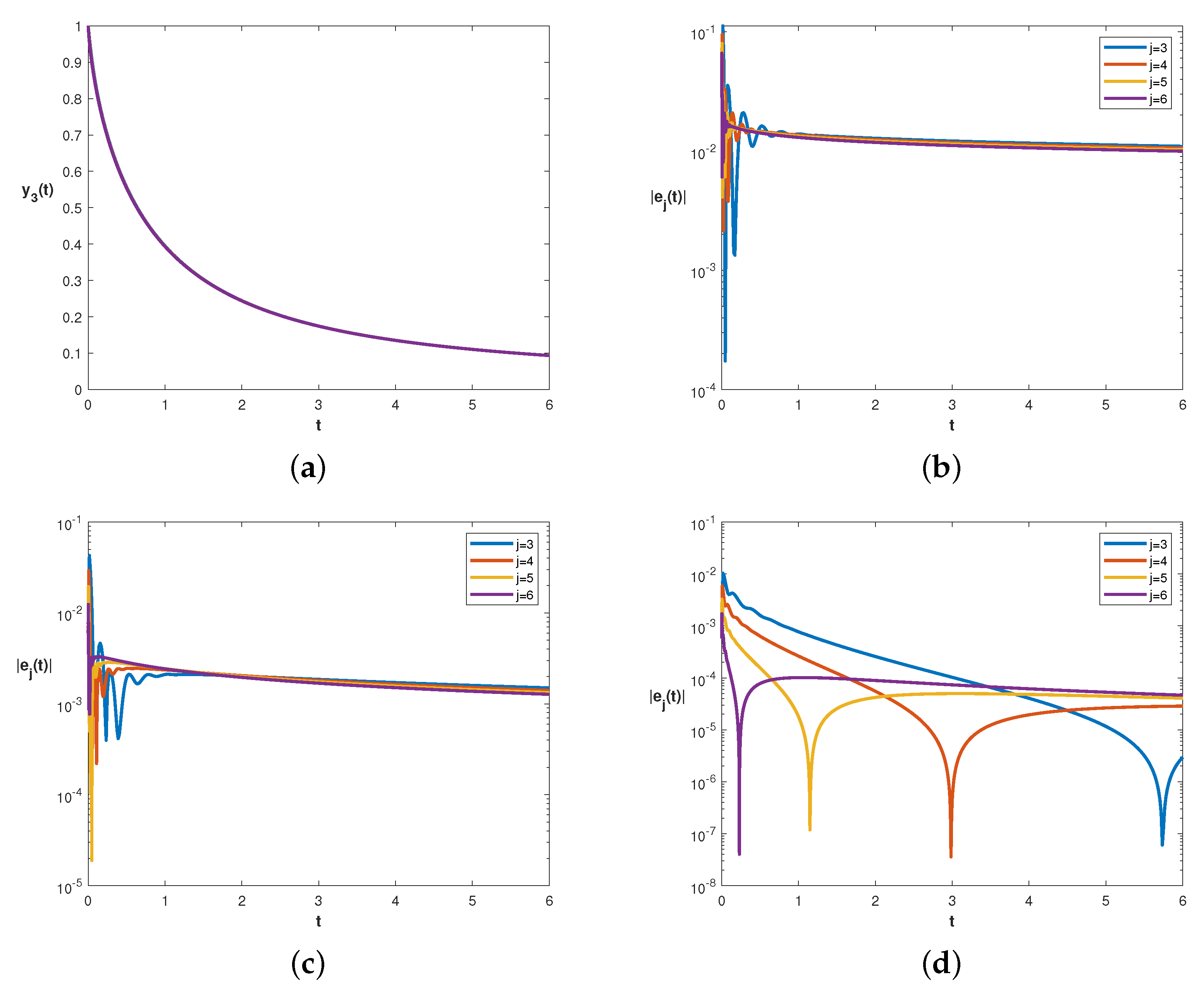
To check the accuracy of the method in the case of large intervals, in the second example, we set the discretization interval to $I=[0,6]$. For this test, we chose $f\left(t\right)\equiv 0$, $b=1$, and $y\left(0\right)=1$, so that the initial value problem (7) becomes:

$$\left\{\begin{array}{c}{{}_{C}D}_t^{\gamma }y\left(t\right)+y\left(t\right)=0,0<t\le 6,0<\gamma <1,\hfill \\ \\ y\left(0\right)=1.\hfill \end{array}\right.$$

One can easily see that in this case, Equation (8) reduces to:

$$y\left(t\right)=E_{\gamma ,1}(-t^{\gamma }).$$

(36)

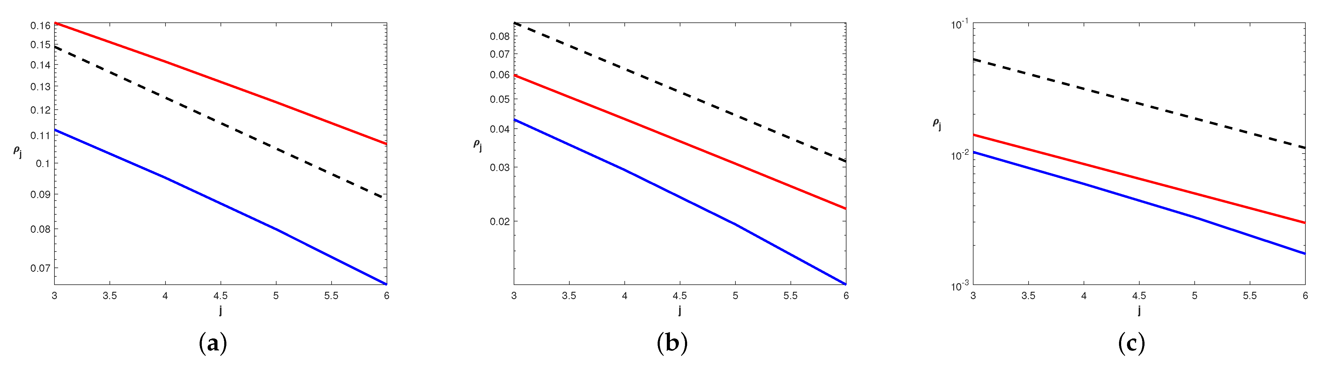
To evaluate the Mittag–Leffler function appearing in the exact solution, we used the algorithm given in [37]. The numerical solution and the absolute value of the error for different values of j and $\gamma$ are displayed in Figure 3. The numerical convergence order is shown in Figure 4. For comparison, a line having the same slope as the theoretical convergence order is also displayed. The infinity norm of the error and the numerical convergence order as a function of the refinement level j are listed in

Table 4. Example 2: The infinity norm of the error and the numerical convergence order for different values of the fractional derivative $\gamma$ and the refinement level j when using $d{Q}_{3j}y$ with $r=1$ (cf. (26)). The number of collocation points is $N_s+1=2^{j}6+1$.

		$\mathit{\gamma }=0.25$		$\mathit{\gamma }=0.5$		$\mathit{\gamma }=0.75$
$\mathit{j}$	${\mathit{N}}_{\mathit{s}}+\mathbf{1}$	$\parallel {\mathit{e}}_{\mathit{j}}{\parallel }_{\infty }$	${\mathit{\rho }}_{\mathit{j}}$	$\parallel {\mathit{e}}_{\mathit{j}}{\parallel }_{\infty }$	${\mathit{\rho }}_{\mathit{j}}$	$\parallel {\mathit{e}}_{\mathit{j}}{\parallel }_{\infty }$	${\mathit{\rho }}_{\mathit{j}}$
3	97	1.61$\times {10}^{-1}$		5.97$\times {10}^{-2}$		1.40$\times {10}^{-2}$
4	193	1.41$\times {10}^{-1}$	0.191	4.29$\times {10}^{-2}$	0.475	8.33$\times {10}^{-3}$	0.744
5	385	1.23$\times {10}^{-1}$	0.199	3.07$\times {10}^{-2}$	0.482	4.97$\times {10}^{-3}$	0.746
6	769	1.07$\times {10}^{-1}$	0.206	2.19$\times {10}^{-2}$	0.488	2.96$\times {10}^{-3}$	0.747

and

Table 5. Example 2: The infinity norm of the error and the numerical convergence order for different values of the fractional derivative $\gamma$ and the refinement level j when using $d{Q}_{3j}y$ with $r=2$ (cf. (27)). The number of collocation points is $N_s+1=2^{j}6+1$.

		$\mathit{\gamma }=0.25$		$\mathit{\gamma }=0.5$		$\mathit{\gamma }=0.75$
$\mathit{j}$	${\mathit{N}}_{\mathit{s}}+\mathbf{1}$	$\parallel {\mathit{e}}_{\mathit{j}}{\parallel }_{\infty }$	${\mathit{\rho }}_{\mathit{j}}$	$\parallel {\mathit{e}}_{\mathit{j}}{\parallel }_{\infty }$	${\mathit{\rho }}_{\mathit{j}}$	$\parallel {\mathit{e}}_{\mathit{j}}{\parallel }_{\infty }$	${\mathit{\rho }}_{\mathit{j}}$
3	97	1.12$\times {10}^{-1}$		4.28$\times {10}^{-2}$		1.03$\times {10}^{-2}$
4	193	9.52$\times {10}^{-1}$	0.236	2.93$\times {10}^{-2}$	0.546	5.88$\times {10}^{-3}$	0.808
5	385	7.98$\times {10}^{-2}$	0.253	1.95$\times {10}^{-2}$	0.588	3.27$\times {10}^{-3}$	0.847
6	769	6.61$\times {10}^{-2}$	0.272	1.24$\times {10}^{-2}$	0.651	1.72$\times {10}^{-3}$	0.926

. Table 4 refers to the quasi-interpolatory operators $d{Q}_{3j}y$ with $r=1$, while Table 5 refers to the case $r=2$.

5. Discussion

The numerical results in Section 4 show that the collocation method we proposed is accurate and efficient. As shown in the first example of Section 4.1, the method is exact for polynomials up to degree $n=3$, the degree of the spline approximating function, so that the error is in the order of the machine precision (cf. Table 1). In the second example of Section 4.1, the error decreases according to the theoretical convergence rate for both quasi-interpolatory operators. In fact, the numerical convergence rate is $O\left(2^{-j\nu }\right)$, where $\nu =2.8$ is the smoothness of the solution $y\left(t\right)=t^{2.8}$ (cf. Table 2 and Table 3). Nevertheless, the quasi-interpolatory operator with $r=2$ gives a smaller error showing that higher accuracy can be achieved by operators with a higher degree of polynomial reproduction. It is worth noting that the error is rather small even at the low refinement level $j=3$, i.e., using only 11 basis functions and 16 collocation points. A similar behavior is shown in the examples of Section 4.2 (cf. Table 4 and Table 5). Here, we used a large discretization interval, i.e., $[0,6]$. We point out that other numerical methods, such as spectral methods or finite difference methods, require high computational cost to approximate accurately the solution of fractional differential equations in large intervals. Instead, our method gives a good accuracy with a low computational cost. In this example, the numerical convergence rate is slightly different from the theoretical one, which is $O\left(2^{-j\nu }\right)$ with $\nu =\gamma$. In particular, the approximation with the quasi-interpolatory operator with $r=1$ shows a lower convergence rate while the quasi-interpolatory operator with $r=2$ shows a higher convergence rate. This behavior is worth investigating in more detail. Finally, we notice that the error is higher near the left boundary (cf. Figure 3). This can be due to the use of truncated B-splines as left-edge functions for which initial conditions are more difficult to fulfil. This problem can be overcome using optimal B-spline bases [38].

The proposed method can be easily applied to more general fractional differential equations. As an example, we consider the Bagley–Torvik equation:

$$\left\{\begin{array}{c}{\displaystyle y^{″}\left(t\right)+{{}_{C}D}_t^{1.5}y\left(t\right)+y\left(t\right)=\frac{15}{4}\sqrt{t}+\frac{15}{8}\sqrt{\pi }t+t^2\sqrt{t},t\in [0,1],}\hfill \\ \\ y\left(0\right)=y^{\prime }\left(0\right)=0,\hfill \end{array}\right.$$

(37)

which is a second order multi-term fractional differential equation used to describe the viscoelastic properties of real materials [39]. Its exact solution is $y\left(t\right)=t^2\sqrt{t}$. We numerically solved Equation (37) using the quasi-interpolatory operator $d{Q}_{nj}y$ with $r=1$ and $r=2$. The infinity norm of the error and the numerical convergence order as a function of the refinement level j are listed in

Table 6. Bagley–Torvik equation: the infinity norm of the error and the numerical convergence order when using $d{Q}_{nj}y$ with $r=1$ (left) and $r=2$ (right).

$\mathit{r}=1$			$\mathit{r}=2$
$\mathit{j}$	$\parallel {\mathit{e}}_{\mathit{j}}{\parallel }_{\infty }$	${\mathit{\rho }}_{\mathit{j}}$	$\mathit{j}$	$\parallel {\mathit{e}}_{\mathit{j}}{\parallel }_{\infty }$	${\mathit{\rho }}_{\mathit{j}}$
3	5.65$\times {10}^{-2}$		3	3.39$\times {10}^{-3}$
4	2.89$\times {10}^{-2}$	0.965	4	1.15$\times {10}^{-3}$	1.564
5	1.48$\times {10}^{-2}$	0.971	5	3.87$\times {10}^{-4}$	1.566
6	7.50$\times {10}^{-3}$	0.977	6	1.30$\times {10}^{-4}$	1.577

. We notice that in the case of differential problems having a second order derivative, the theoretical convergence order is smaller than $O\left(2^{-j\nu }\right)$, as the numerical results show. The error is comparable with the error obtained by other spline methods in the literature (cf. [20,22]) and shows that the method is effective also for this kind of problem. More general problems, such as boundary value problems and nonlinear problems, will be the subject of a forthcoming paper.

6. Conclusions

The numerical method presented in this paper combines collocation methods and spline quasi-interpolatory operators involving divided differences to approximate the solution to a linear time fractional differential equation. The method is convergent and reproduces polynomials of suitable degree. The numerical tests confirm the theoretical results and show that the accuracy of the method can be improved using quasi-interpolatory operators reproducing polynomials of higher degree.

The use of the proposed method to solve nonlinear fractional differential equations is at present under study. Moreover, we aim to improve the accuracy of the method by using optimal spline bases and different kinds of quasi-interpolatory operators.