Fractional-Order PI Controller Design Based on Reference–to–Disturbance Ratio

Abstract

The presence of disturbances in practical control engineering applications is unavoidable. At the same time, they drive the closed-loop system’s response away from the desired behavior. For this reason, the attenuation of disturbance effects is a primary goal of the control loop. Fractional-order controllers have now been researched intensively in terms of improving the closed-loop results and robustness of the control system, compared to the standard integer-order controllers. In this study, a novel tuning method for fractional-order controllers is developed. The tuning is based on improving the disturbance attenuation of periodic disturbances with an estimated frequency. For this, the reference–to–disturbance ratio is used as a quantitative measure of the control system’s ability to reject disturbances. Numerical examples are included to justify the approach, quantify the advantages and demonstrate the robustness. The simulation results provide for a validation of the proposed tuning method.

1. Introduction

Disturbances are considered to be unknown, unpredictable, unmodeled or uncertain factors that drive the closed-loop system’s response away from the desired behavior. Disturbances also occur frequently in control systems. Due to their negative impact, a major concern regarding the controller design is focused on achieving an adequate degree of disturbance rejection. The authors of [1] classify disturbances into two main categories: endogenous and exogenous. The endogenous class depends on internal variables of the controlled system such as nonlinearities, various states, outputs or unmodeled characteristics. The exogenous disturbances are defined as any unwanted phenomena, which are caused by the external environment, such as other systems that interact with the controlled process. The focus of this study is on exogenous periodic disturbances acting on the plant input, whose frequency can be estimated as ω_d.

A deterministic method to assess the disturbance rejection ability of a control system has been defined in [2]. The reference–to–disturbance ratio (RDR) was defined similarly to the signal–to–noise ratio in communication channels. As such, the RDR represents a quantitative measure regarding the input dominancy on disturbance at the system output. For satisfactory disturbance rejection performance, a control system should have an RDR >> 1. If RDR << 1, the control system does not exhibit any disturbance attenuation [2]. Considering the generalized closed-loop control system in Figure 1, the authors of [2] defined the spectral power of reference signal at the output of the closed-loop system as

$${\left|y_r\left(j\omega \right)\right|}^2={\left|\frac{H_c\left(j\omega \right)H_p\left(j\omega \right)}{1+H_c\left(j\omega \right)H_p\left(j\omega \right)}\right|}^2{\left|r\left(j\omega \right)\right|}^2$$

(1)

where $y_r$ is the output signal corresponding to a change in the reference signal $r$, H_c is the controller transfer function, H_p is the process transfer function and $\omega$ is the frequency.

The spectral power of the disturbance signal d at the output of the closed-loop system was expressed as

$${\left|y_d\left(j\omega \right)\right|}^2={\left|\frac{H_p\left(j\omega \right)}{1+H_c\left(j\omega \right)H_p\left(j\omega \right)}\right|}^2{\left|d\left(j\omega \right)\right|}^2$$

(2)

where $y_d$ is the output signal corresponding to a change in the disturbance signal $d$.

Similar to signal–to–noise ratio, the RDR is defined as

$$\mathrm{RDR}\left(\omega \right)=\frac{{\left|y_r\left(j\omega \right)\right|}^2}{{\left|y_d\left(j\omega \right)\right|}^2}$$

(3)

For a fair comparison, the two input signals are considered to have equal powers: ${\left|r\left(j\omega \right)\right|}^2$=${\left|d\left(j\omega \right)\right|}^2$. Then, replacing (1) and (2) into (3) leads to

$$\mathrm{RDR}\left(\omega \right)={\left|H_c\left(j\omega \right)\right|}^2$$

(4)

As can be seen in (4), the ability to suppress disturbances depends solely on the energy spectral density of the controller transfer function. Thus, designing the controller in order to maximize the RDR value, leads to improved closed-loop disturbance rejection. In [2], the authors analyze and test the theoretical results regarding the RDR for Proportional Integral Derivative (PID) controllers, as well as for the Fractional-Order PIDs (FO-PID). This study is focused solely on FO-PIDs [3]. These are generalizations of the standard PID controllers, with the transfer function defined as

$$H_{\mathrm{PID}}\left(s\right)=k_p\left(1+k_i{s}^{-\lambda }+k_d{s}^{\mu }\right)$$

(5)

where k_p, k_i and k_d are the proportional, integral and derivative gains. $\lambda ϵ\left[0, 1\right]$ and $\mu ϵ\left[0, 1\right]$ represent the fractional orders of integration and differentiation, respectively. Using (4) and (5), it follows that there is a frequency dependence of the RDR spectrum on the fractional orders $\lambda$ and $\mu$ [2].

Research on FO-PID controllers, regarding their advantages compared to the traditional PID controllers as well as tuning methods, is currently a major trend in control engineering. Numerous papers have shown that FO-PIDs lead to better closed-loop performance, as well as increased robustness [4,5,6]. Most tuning methods for these controllers use the frequency representation of the process and controller, while the performance specifications are expressed also in the frequency domain: gain crossover frequency ${\omega }_c$, phase margin PM, gain margin GM, etc. In this study, also, the frequency representation is preferred. However, apart from the gain crossover frequency and phase margin, the RDR measure is also used as a performance specification.

The scarcity of literature targeting RDR as a tuning parameter motivates the development of the proposed tuning strategy. The present paper contributes to the control engineering field by providing a novel tuning procedure, consisting of an adaptation of the most popular tuning methodology for fractional-order controllers, targeting frequency domain specifications of the open loop system. The novelty of the work lies in directly embedding the RDR value as an explicit control specification, ensuring an intrinsic controller ability to successfully reject periodic disturbances, without the usage of any additional structure or complex mathematical optimization algorithms.

The paper is structured as follows. After this brief introductory section, a generalized overview of disturbance rejection in control engineering is given. Then, the tuning method for FO-PI controllers based on the RDR is detailed in the third section. The fourth section presents some numerical examples to validate the proposed tuning method, as well as its advantages. The final section includes some concluding remarks.

2. Disturbance Rejection in Control Engineering

The presence of disturbances in practical control engineering applications is unavoidable. Hence, the attenuation of disturbance effects is a primary goal of the control loop. Existing control strategies focus on disturbance rejection from explicit and implicit points of view. Explicit approaches involve the engagement of additional blocks such as filters [7,8], state observers [7,9], disturbance estimators [10,11], or even robust adaptive feedback controllers [12,13]. All these blocks contribute to an increased complexity of the control loop with multiple disadvantages from tuning and practical implementation points of view.

A simpler approach consists of implicit control strategies, which inherently rejects disturbances. A manifold of implicit control strategies has been developed that directly address the disturbance rejection performance as a tuning parameter. For example, disturbance rejection is used in the tuning methodology as a frequency domain specification in [14] targeting time delay systems and in [15] for decoupling and pole placement. Furthermore, works such as [16,17,18,19] prove that minimizing the sensitivity function as a tuning parameter is also a popular approach in dealing with disturbance rejection performance, especially for fractional-order control strategies. Another popular approach throughout the specialized literature is high-gain feedback control, proving especially useful in the case of unknown disturbances, which are not accessible for measurement [20,21,22,23].

Another technique that has gained popularity in recent years is the Active Disturbance Rejection Control (ADRC). The strategy is a model-free control that treats both types of disturbances, endogenous and exogenous, as a single, unified, framework. The lumped effects of the disturbance drastically simplify the process to be controlled, which represents both an advantage and a disadvantage at the same time. Practitioners successfully use ADRC methods in real life control implementations [24,25,26], but the method is highly criticized by the mathematically oriented control community [27,28,29,30]. The canonical form of the system and the state observer are employed in ADRC concepts, the method presenting a versatile tuning procedure with multiple advances in different tuning directions. ADRC has also been implemented conjointly with fractional calculus in various applications, extending the performance of fractional-order controllers for disturbance rejection scenarios [31,32].

For some cases, the presence of disturbances is not taken into consideration in the tuning procedure as an explicit specification, but some controllers are able to obtain disturbance rejection through their nature. Such an example is the popular PID controller, which uses the integrator effect to keep a zero steady-state error, leading to disturbance rejection, even if the performance in this area may be suboptimal. Since most processes are subjected to disturbances in various ways, especially in practical control implementations, disturbance rejection is assessed in almost every closed-loop system’s performance. Some works such as [33,34,35] validate the performance of the controller to disturbance rejection scenarios by analyzing the system’s response using experimental tests.

A different approach is the disturbance performance assessment through a series of markers, providing mathematical insight into the abilities of the closed-loop system to eliminate the effects of unwanted interactions. The RDR provides a spectral dependence measurement of the reference signal energy with respect to disturbance signal energy, giving a straightforward analytical method to measure the disturbance rejection capacity of a system [2]. Even if RDR has proven to be an accurate description of a system’s disturbance rejection capability, the concept is rather new in controller tuning approaches. There are few works available that use the ratio in the tuning procedure, rather than an analysis metric. In [36], the authors use the period of the RDR signal with respect to the sampling time and aim at keeping this value constant with two approaches. The first proposal targets the real-time adaptation of the sampling time with respect to the RDR value and performing stability studies using LMI methods in robust control techniques. The second method introduces a new compensator structure that forces the behavior of the closed-loop process to follow a predefined pattern, eliminating the effect of the variable sampling. The study somehow targets RDR as a tuning knob, even if it does not use it as a pure design specification, but rather as an additional factor for non-uniform frequencies, combined with an additional block in an explicit disturbance rejection compensator.

The authors of [37] tune a Fractional-Order Proportional Integral Derivative Acceleration (FOPIDA) through a proposed Consensus-Oriented Random Search (CORS) algorithm that implements a consensus curve that shows the design tradeoff between the reference and disturbance values. RDR is used as one of the multiple factors that contribute to the numerical optimization leading to the FOPIDA controller. The CORS algorithm is a complex design methodology, requiring a multi-step approach in the control design procedure, starting from an initial configuration of a possible candidate for the FOPIDA controller and also employing the use of additional filters to reach the control objective. A graphical tuning algorithm is proposed in [38] that develops an integer-order PID controller that improves the RDR parameter. Various parameters are selected for the PID controller in order to provide a stable and robust closed-loop system using the Specifications-Oriented Kharitonovn Region (SOKR). The method is shown to be versatile, but the graphical approach is more focused on stability and robustness, rather than on the RDR ratio. Furthermore, the usage of SOKR in tuning is not a popular choice throughout the control community. An extensive analysis regarding the effects of FO-PI controller parameters with respect to the RDR value has been presented in [39]. The authors use RDR to assess the disturbance rejection capability of a closed-loop system equipped with an FO-PI controller, tuned without any regard to RDR, by varying the proportional and integral gains of the controller. The study proves that good disturbance rejection performance can be obtained using the FO-PI controller, if the parameters of the controller are properly chosen.

3. Tuning FO-PI Controllers Based on the RDR

In this section, the tuning of fractional-order controllers according to the proposed approach is presented. Three performance specifications are considered, which can be used to tune three parameters of a fractional-order controller. Hence, the proposed method is suitable for FO-PI, FOPD and the FO-PID controller in (5). In the latter case, the method can be used if $\lambda$ = $\mu$ and k_i = r · k_d, where r is a user-selected ratio between the integral and derivative gains. In the remainder of the section, only details regarding the tuning of an FO-PI controller are presented, but the equations can be easily extended for the other cases mentioned above. The FO-PI controller was chosen due to its inherent ability to ensure zero steady-state errors.

The performance specifications are given as gain crossover frequency ${\omega }_c$, phase margin PM and maximum RDR for an estimated disturbance frequency ${\omega }_d$. The gain crossover frequency ensures a certain settling time of the overall closed-loop system, where the larger the ${\omega }_c$, the faster the system will reach steady-state values. The phase margin ensures a certain overshoot for the closed-loop system. The large the PM is, the smaller the overshoot is. The maximization of RDR at a specific disturbance frequency implies better periodic disturbances attenuation around that frequency. To also ensure zero tracking errors, a fractional-order PI controller is proposed, defined as

$$H_c\left(s\right)=k_p\left(1+k_i{s}^{-\lambda }\right)$$

(6)

Its frequency representation is given as

$$H_c\left(j\omega \right)=k_p\left(1+k_i{\omega }^{-\lambda }\left(\cos \frac{\lambda \pi }{2}-j·\sin \frac{\lambda \pi }{2}\right)\right)$$

(7)

Having the modulus and phase at the gain crossover frequency

$$\angle H_c\left(j{\omega }_c\right)=-{\tan }^{-1}\frac{k_i{\omega }_c^{-\lambda }\sin \frac{\lambda \pi }{2}}{1+k_i{\omega }_c^{-\lambda }\cos \frac{\lambda \pi }{2}}$$

(8)

$$\left|H_c\left(j{\omega }_c\right)\right|=k_p\sqrt{k_i^2{\omega }_c^{-2\lambda }+1+2k_i{\omega }_c^{-\lambda }\cos \frac{\lambda \pi }{2}}$$

(9)

For a general process transfer function, H_p(s), the modulus and phase of the process are computed at the required gain crossover frequency and denoted as $\left|H_p\left(j{\omega }_c\right)\right|$ and $\angle H_p\left(j{\omega }_c\right)$, respectively.

The performance criteria regarding the open loop gain crossover frequency and phase margin lead to the following equations:

$$\angle H_p\left(j{\omega }_c\right)+\angle H_c\left(j{\omega }_c\right)=-\pi +PM$$

(10)

$$\left|H_p\left(j{\omega }_c\right)\right|·\left|H_c\left(j{\omega }_c\right)\right|=1$$

(11)

which lead to

$${\tan }^{-1}\frac{k_i{\omega }_c^{-\lambda }\sin \frac{\lambda \pi }{2}}{1+k_i{\omega }_c^{-\lambda }\cos \frac{\lambda \pi }{2}}=\pi -PM+\angle H_p\left(j{\omega }_c\right)$$

(12)

and

$$\left|H_p\left(j{\omega }_c\right)\right|·k_p\sqrt{k_i^2{\omega }_c^{-2\lambda }+1+2k_i{\omega }_c^{-\lambda }\cos \frac{\lambda \pi }{2}}=1$$

(13)

Equation (12) can now be used to determine the integral gain k_i as a function of the fractional order $\lambda$:

$$k_i=\frac{\tan \left(\pi -PM+\angle H_p\left(j{\omega }_c\right)\right){\omega }_c^{\lambda }}{\sin \frac{\lambda \pi }{2}-\tan \left(\pi -PM+\angle H_p\left(j{\omega }_c\right)\right)\cos \frac{\lambda \pi }{2}}$$

(14)

Similarly, Equation (13) can be used to determine the proportional gain k_p as a function of the fractional order $\lambda$:

$$k_p=\frac{1}{\left|H_p\left(j{\omega }_c\right)\right|\sqrt{k_i^2{\omega }_c^{-2\lambda }+1+2k_i{\omega }_c^{-\lambda }\cos \frac{\lambda \pi }{2}}}$$

(15)

Using (4), the RDR for an FO-PI controller is defined as follows:

$$\mathrm{RDR}\left({\omega }_d\right)=k_p^2\left(k_i^2{\omega }_d^{-2\lambda }+1+2k_i{\omega }_d^{-\lambda }\cos \frac{\lambda \pi }{2}\right)$$

(16)

where ${\omega }_d$ is the estimated frequency of the sinusoidal disturbance. The scope of the design is to determine the controller parameters in (6) such that the RDR is maximized. The procedure is an iterative one. The algorithm is given in Figure 2.

4. Numerical Examples

Six numerical examples are provided for simple, higher order, integrating and unstable processes. However, the design procedure can be easily applied to any process, even fractional-order systems. Firstly, a justificative example is included to demonstrate that the RDR can be modified based on the fractional order. Then, we show through a first-order process that in certain situations, fractional-order controllers designed according to the proposed RDR maximization method ensure better closed-loop performance compared to their integer-order counterparts. A first-order plus dead-time process is used to demonstrate that, based on the RDR maximization, better robustness to disturbance frequency variations can be achieved. A fourth example for a higher-order process is considered. A comparison is performed with an FO-PI that was tuned in order to meet the same phase margin and gain crossover frequency. The fifth example considers an integrating system. Several existing tuning methods for FO controllers are considered as comparisons. For a realistic approach, noisy signals are considered in the simulations. The last numerical example is an unstable system. The numerical simulations show that even in this case, the proposed approach ensures better attenuation of periodic disturbances, compared to some optimally tuned FO-PIDs, as well as a PID controller.

In all examples, the selection of the performance specifications referring to the gain crossover frequency and phase margin is made according to the rules indicated in [40].

4.1. Justificative Example

For the process described by

$$H_p\left(s\right)=\frac{0.5}{4s+1}$$

(17)

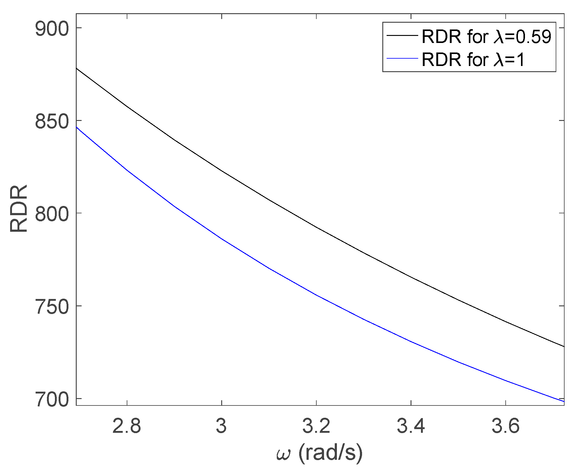
that could describe the dynamics of a DC motor, the following performance specifications are imposed: PM = 60° and ${\omega }_c=8$ rad/s. To illustrate the importance of maximizing the RDR for the disturbance rejection property, two values for the fractional order are randomly selected as ${\lambda }_1=0.4$ and ${\lambda }_2=0.9$. The integral gain is then computed according to the phase margin criteria in (14), while k_p is determined based on the magnitude equation in (15). The RDR is then evaluated at a frequency of interest ${\omega }_d=0.8$ rad/s, resulting in ${\mathrm{RDR}}_{{\lambda }_1}=2.27\times {10}^4$ and ${\mathrm{RDR}}_{{\lambda }_2}=8.02\times {10}^4$ and, thus, a ratio $\frac{{\mathrm{RDR}}_{{\lambda }_2}}{{\mathrm{RDR}}_{{\lambda }_1}}=3.53$. This suggests that a better disturbance rejection can be achieved using an FO-PI controller with $\lambda =0.9$, k_p = 49.08 and k_i = 4.52.

Figure 3 shows the resulting RDR values for a frequency range $\omega \in \left(0.1÷1.5\right)$ rad/s, thus including the estimated disturbance frequency ${\omega }_d$. It is obvious from this figure that larger values for the RDR are obtained in this frequency range for the FO-PI controller with $\lambda =0.9$. In fact, the lower the disturbance frequencies, the better the rejection improvement.

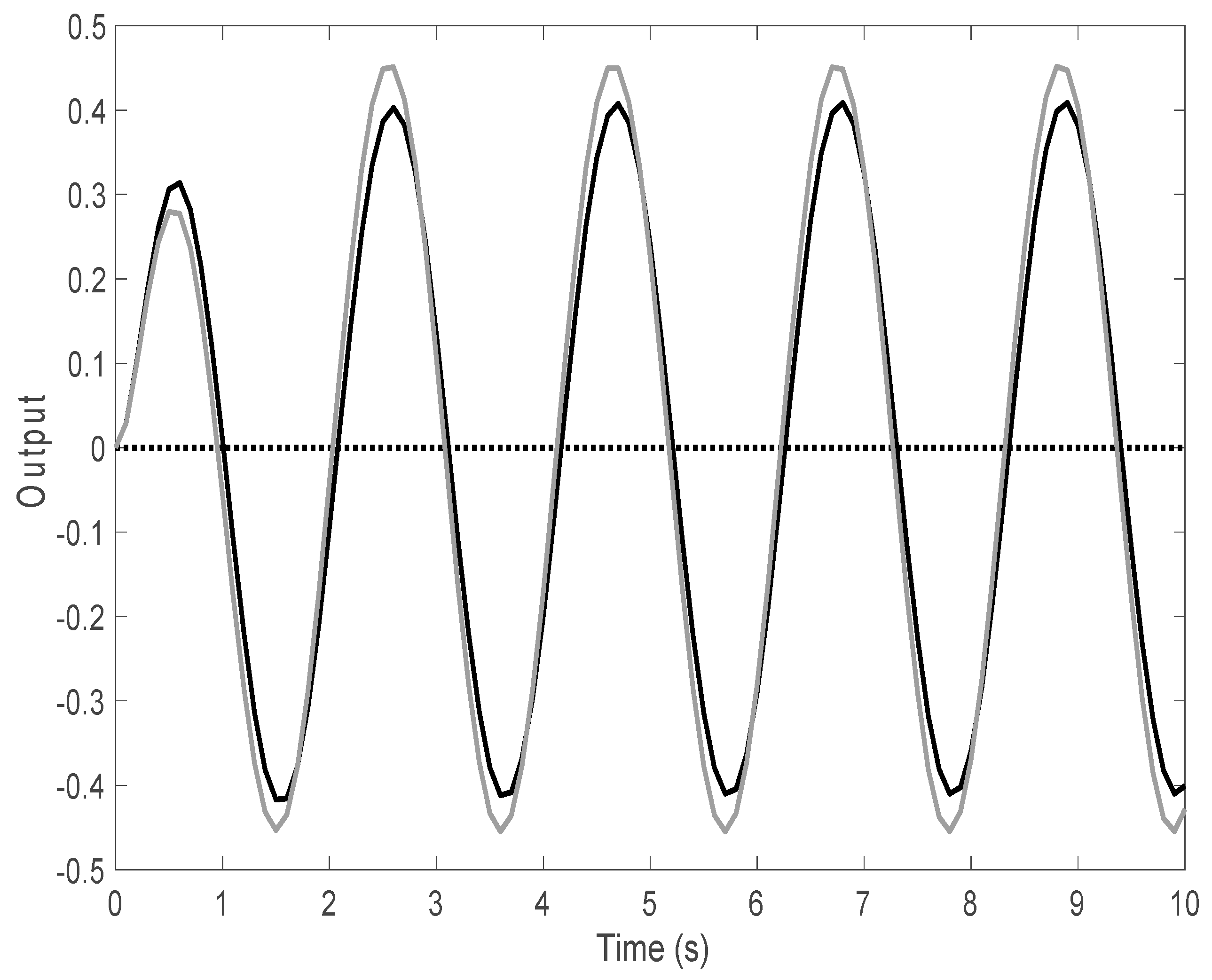
The disturbance rejection results in Figure 4 and Figure 5 demonstrate that better disturbance attenuation is achievable using the FO-PI with $\lambda =0.9$, compared to the FO-PI with $\lambda =0.4$. The two controller transfer functions are:

$$H_{FO\_P{I}_{{\lambda }_1}}\left(s\right)=8\left(1+16.48s^{-0.4}\right)$$

(18)

$$H_{FO\_P{I}_{{\lambda }_2}}\left(s\right)=49.08\left(1+4.52s^{-0.9}\right)$$

(19)

To implement the FO-PI controllers, the Non-Rational Transfer Function (NRTF) discrete-time approximation method is used [41], with N = 5, $\alpha =0.5$ and $T_s=0.02 \mathrm{s}$, where N is the order of the approximation, $\alpha$ is a tuning knob and T_s is the sampling period. The FO-PI controllers are thus approximated to discrete-time higher-order transfer functions. As suggested in [41], the order N = 5 is considered a suitable choice for producing an accurate discrete-time approximation of fractional-order systems. For the simulations presented in Figure 4 and Figure 5, the reference signal was kept at 0, with the disturbance amplitude selected to be 2 and its frequency equal to $0.8$ rad/s (Figure 4) and $0.2$ rad/s (Figure 5). The maximum output amplitude is taken as a quantitative measure of the FO-PI controller performance. In the case of the disturbance frequency being equal to the design frequency ${\omega }_d$ (Figure 4), an improvement of 43% is obtained by using the FO-PI controller with $\lambda =0.9$, with the FO-PI thus tuned based on the proposed approach. In the case of Figure 5, the improvement is nearly 70%.

4.2. Improved Disturbance Rejection of FO Controllers Compared to Integer-Order (IO) Controllers Based on the RDR Measure

The design procedure based on Figure 2 is described in what follows for a process similar to (17):

$$H_p\left(s\right)=\frac{1}{5s+1}$$

(20)

which could describe the dynamics of a DC motor; the following performance specifications are imposed: PM = 70° and ${\omega }_c=5$ rad/s. The integral gain k_i is then computed according to (14) for $\lambda \in \left(0÷1\right)$. The proportional gain k_p is then determined based on (15) for each pair ($\lambda$, k_i). The RDR is then evaluated at a frequency of interest ${\omega }_d=3$ rad/s, and the result is given in Figure 6.

According to Figure 6, the maximum RDR value is obtained for $\lambda =0.59$; thus, k_i = 1.91 and k_p = 16.02. Additionally, based on Figure 6, it is obvious that for a disturbance signal with frequency ${\omega }_d=3$ rad/s, the FO-PI controller (with RDR_FO-PI = 822) is more efficient in rejecting the disturbance compared to a traditional PI controller (with RDR_PI = 786).

Figure 7 demonstrates that a similar conclusion is valid if the disturbance signal frequency is centered in a frequency band $\omega \in \left(2.5÷3.7\right)$ rad/s. To implement the FO-PI controller, the NRTF approach is used [41], with N = 5, $\alpha =0.9$ and $T_s=0.1 \mathrm{s}$, where N is the order of the approximation, $\alpha$ is a tuning knob and T_s is the sampling period. As suggested in [41], the order N = 5 is considered a suitable choice for producing an accurate discrete-time approximation of fractional-order systems.

The closed-loop simulation results for reference tracking are indicated in Figure 8. Although not directly tackled, the FO-PI achieves a smaller overshoot and an improved settling time compared to the traditional PI. The FO-PI controller achieves an overshoot of 17%, while the overshoot obtained with the PI controller is larger, 23%. A slightly faster settling time of 1.1 s is also obtained with the FO-PI controller, compared to the 1.4 s achieved using the PI.

Figure 9 shows the disturbance rejection results, considering a sinusoidal disturbance of unit amplitude and frequency ${\omega }_d=3$ rad/s. The FO-PI manages to reduce the amplitude of the signal, compared to the PI, since the RDR is higher in the case of the FO-PI controller. The percent improvement is small, 12%, but corresponds to the RDR values associated to the two controllers, RDR_FO-PI/RDR_PI = 1.045. A higher RDR ratio will produce a larger percent improvement in the attenuation of the periodic signal, as illustrated in the previous example.

4.3. A First-Order plus Dead-Time Process for Robustness Analysis of the Design

For the process described by

$$H_p\left(s\right)=\frac{0.05}{2s+1}{e}^{-0.7s}$$

(21)

the following performance specifications are imposed: PM = 60° and ${\omega }_c=1$ rad/s. The integral gain k_i is then computed according to (14) for $\lambda \in \left(0÷1\right)$. The proportional gain k_p is then determined based on (15) for each pair ($\lambda$, k_i). The RDR is then evaluated at a frequency of interest ${\omega }_d=0.5$ rad/s, and the result is given in Figure 10.

According to Figure 10, the maximum RDR value is obtained for $\lambda =0.83$; thus, k_i = 0.6 and k_p = 34.58. To implement the FO-PI controller, the NRTF approach is used [41], with N = 5, $\alpha =0.9$ and $T_s=0.2 \mathrm{s}$. The closed-loop simulation results for reference tracking are indicated in Figure 11. In this case, the overshoot is 25%, and the settling time is 20 s. Figure 12 shows the disturbance rejection results, considering a sinusoidal disturbance of unit amplitude and frequency ${\omega }_d=0.5$ rad/s. A sinusoidal reference signal of unit amplitude and frequency $\omega =0.02$ rad/s is also used. The results show that the method is effective in dealing with the disturbance signal. To test the robustness of the disturbance rejection property, two disturbance signals with frequencies ${\omega }_d/2$ and ${\omega }_d\ast 2$, respectively, are used.

The simulation results are indicated in Figure 13. The mean-squared errors for the disturbance rejection results are 4.52, 5.81 and 4.10, for the case of sinusoidal disturbance signals of frequencies ${\omega }_d$, ${\omega }_d\times 2$ and ${\omega }_d/2$, respectively. This result is in accordance with the RDR values in Figure 14 for the current proposed controller, where ${\mathrm{RDR}}_{{\omega }_d}=3215$, ${\mathrm{RDR}}_{{\omega }_d\ast 2}=2000$ and ${\mathrm{RDR}}_{{\omega }_{d/2}}=$ 6650. The higher the disturbance frequency, the poorer the attenuation.

4.4. The Counterexample

A counterexample is included here as well. For the same process in (21), an FO-PI controller is designed with $\lambda =0.5$; thus, k_i = 1.4 and k_p = 20.11. To implement the FO-PI controller, the NRTF approach is used [41], with N = 5, $\alpha =0.9$ and $T_s=0.2 \mathrm{s}$. In this case, as Figure 10 shows, the RDR value is smaller than the RDR value for $\lambda =0.83$, chosen as the maximum. Figure 15 shows the disturbance rejection results using this new controller and a sinusoidal disturbance signal of unit amplitude and frequency ${\omega }_d=0.5$ rad/s. A sinusoidal reference signal of unit amplitude and frequency $\omega =0.02$ rad/s is used. Sinusoidal disturbance signals of unit amplitude and frequencies ${\omega }_d\ast 2$ and ${\omega }_d/2$ are also considered. The simulation results are given in Figure 15. The mean-squared errors for the disturbance rejection results are 18.53, 20.21 and 18.23, for the case of sinusoidal disturbance signals of frequencies ${\omega }_d$, ${\omega }_d\ast 2$ and ${\omega }_d/2$, respectively. Comparing this with the previous results obtained with the FO-PI controller designed according to RDR maximization gives 75.6%, 71.25% and 77.5% improvement obtained with the proposed FO-PI controller. This demonstrates yet again the efficiency of the proposed method, even in terms of the robustness to disturbance frequency variations.

4.5. A Higher-Order Process with Delay Dominance

A comparison with a Ziegler–Nichols derived tuning method for FO-PI controllers is used to compare the results. The simulation results are intended to show that maximizing the RDR value, along with other performance specifications, leads to better disturbance rejection, as well as similar reference tracking performance. A higher-order process is considered [42]:

$$H_p\left(s\right)=\frac{1}{{\left(s+1\right)}^4}$$

(22)

An FO-PI has been designed in [42], with the parameters k_p = 0.61, k_i = 28 and $\lambda =1.13$. This FO-PI achieves a PM = 65° and ${\omega }_c=0.46$ rad/s. The same performance specifications are used to design an FO-PI controller using the proposed method. The integral gain k_i is then computed according to (14) for $\lambda \in \left(0÷1\right)$. The proportional gain k_p is then determined based on (15) for each pair ($\lambda$, k_i). The RDR is then evaluated at a frequency of interest ${\omega }_d=0.2$ rad/s, and the result is given in Figure 16. The maximum RDR value is obtained for $\lambda =0.89$; thus, k_i = 0.26 and k_p = 1.08. The performance of the proposed FO-PI controller is compared to that obtained using [42]. To implement the two FO-PI controllers, the NRTF approach is used [41], with N = 5, $\alpha =0.9$ and $T_s=0.2 \mathrm{s}$.

The closed-loop simulation results for reference tracking are indicated in Figure 17. In this case, the overshoot is 3.4%, and the settling time is 36.1 s. The overshoot obtained with the FO-PI designed according to [42] is 6.3%, while the settling time is 34.1 s. The simulation results indicate that similar results can be obtained using the proposed method. However, the main target of the proposed approach is directed towards the maximization of RDR, which should allow for better disturbance rejection.

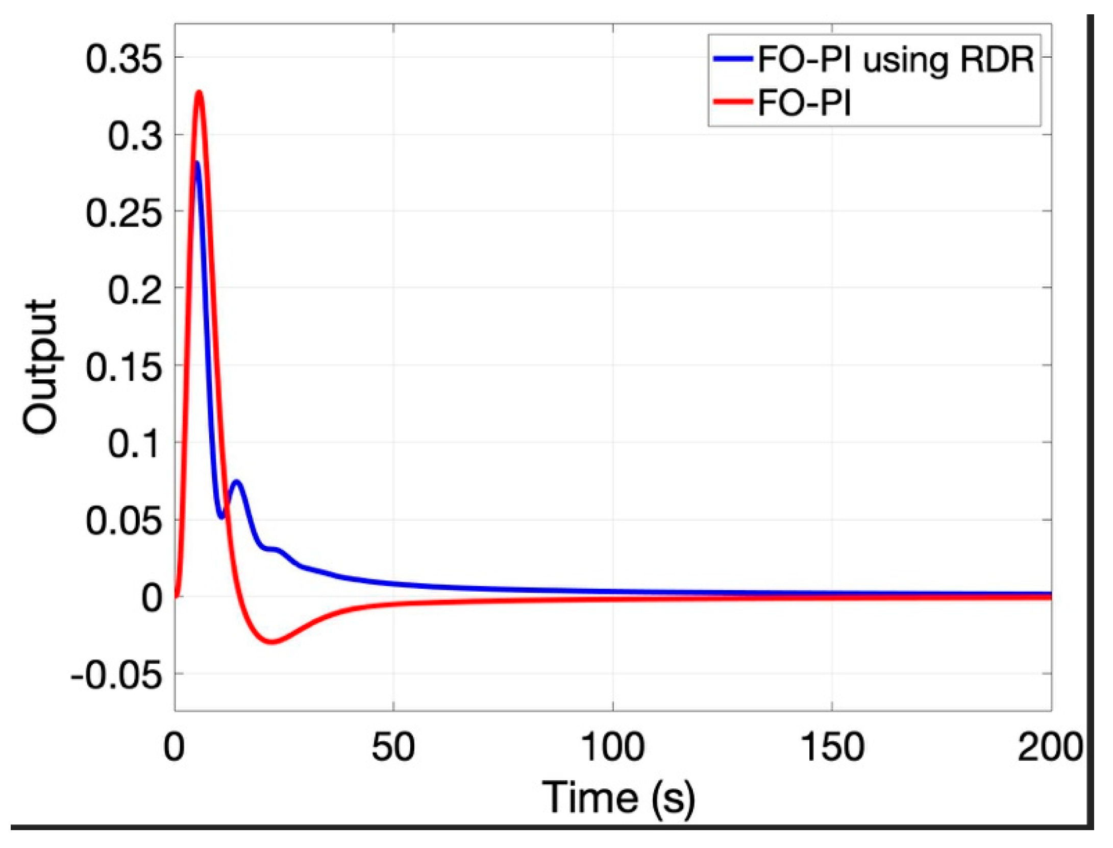
Figure 18 shows the disturbance rejection results, considering a sinusoidal disturbance of 0.2 amplitude and frequency ${\omega }_d=0.2$ rad/s. The reference signal is assumed to be 0. The maximum amplitude at the output, using the FO-PI controller in [42], is 0.184, whereas the maximum amplitude with the proposed FO-PI controller is kept at 0.1. This suggests a 45.6% improvement, due to the maximization of the RDR value for this specific disturbance frequency. The mean-squared error obtained using the proposed method is 20.71, whereas the mean-squared error obtained using the FO-PI in [42] is 61.26. This leads to a 66.2% improvement in rejecting the sinusoidal disturbance.

A load disturbance of amplitude 0.5 is also considered for comparison purposes. Figure 19 shows the simulation results, considering this disturbance and a reference signal equal to 0. In this case also, although not directly tackled, the proposed method ensures good load disturbance rejection, with a smaller output amplitude and a similar disturbance rejection time. The mean-squared errors in the two cases are 6.62 using the proposed method and 10.06 using the FO-PI designed according to [42], resulting in 34.2% improvement.

Lastly, a swept sine of amplitude 0.2 and frequency ranging [$0.5{\omega }_d, 2{\omega }_d$] is considered, and the comparative simulation results are given in Figure 20. The mean-squared error in this case is 62.9 for the proposed method and 159.91 for the FO-PI designed using [42]. This accounts for 60.6% improvement in attenuating stochastically varying disturbances.

4.6. An Integrating Process

An integrating time delay process is considered as a fifth example [43]:

$$H_p\left(s\right)=\frac{0.2}{s\left(0.5s+1\right)}$$

(23)

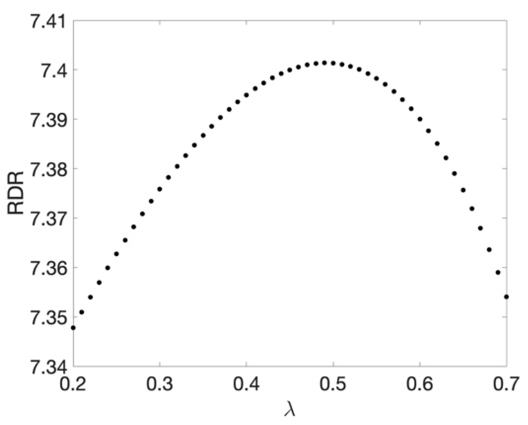
To design the FO-PI controller using the proposed method, a PM = 70° and ${\omega }_c=0.5$ rad/s are imposed, as well as the maximization of the RDR. Figure 21 displays the RDR value as a function of the fractional-order $\lambda$, for a disturbance frequency ${\omega }_d=0.1$ rad/s. The maximum value for the RDR = 7.4 is obtained for $\lambda$ = 0.48. This then results in k_i = 0.04, computed using (14), and k_p = 2.52, computed according to (15).

The performance of the proposed FO-PI controller is compared to the performance of several other fractional-order controllers. The default controller, designed specifically for the process in (23), is an FO-PID consisting of an FO-PI in series with an FO-PD [43]:

$$C_{MONJE}\left(s\right)={\left(\frac{0.4348s+1}{s}\right)}^{1.1803}{\left(\frac{3.7282s+1}{0.0037s+1}\right)}^{1.1580}$$

(24)

Three other fractional-order controllers are designed: two FO-PIDs computed using two different Ziegler–Nichols tuning rules [44,45] and an FO-PI tuned according to the well-known method that ensures the iso-damping property [6]. The parameters of these controllers are included in

Table 1. FO-PID controllers for the integrative time delay process.

Controller Type	kp	ki	$\mathit{\lambda }$	kd	$\mathit{\mu }$
FO-PID ZN-FOC [44]	5.9002	0.3737	0.4	1.5242	0.4
FO-PID ZN-FOC [45]	1.0342	0.943	1.0827	0.8148	0.7855
FO-PI [6]	0.3812	0.3573	0.71	-	-

. All controllers were implemented using the same NRTF approach [41], as well as the same parameters for the approximation with N = 5, $\alpha =0.9$ and $T_s=0.2 \mathrm{s}$.

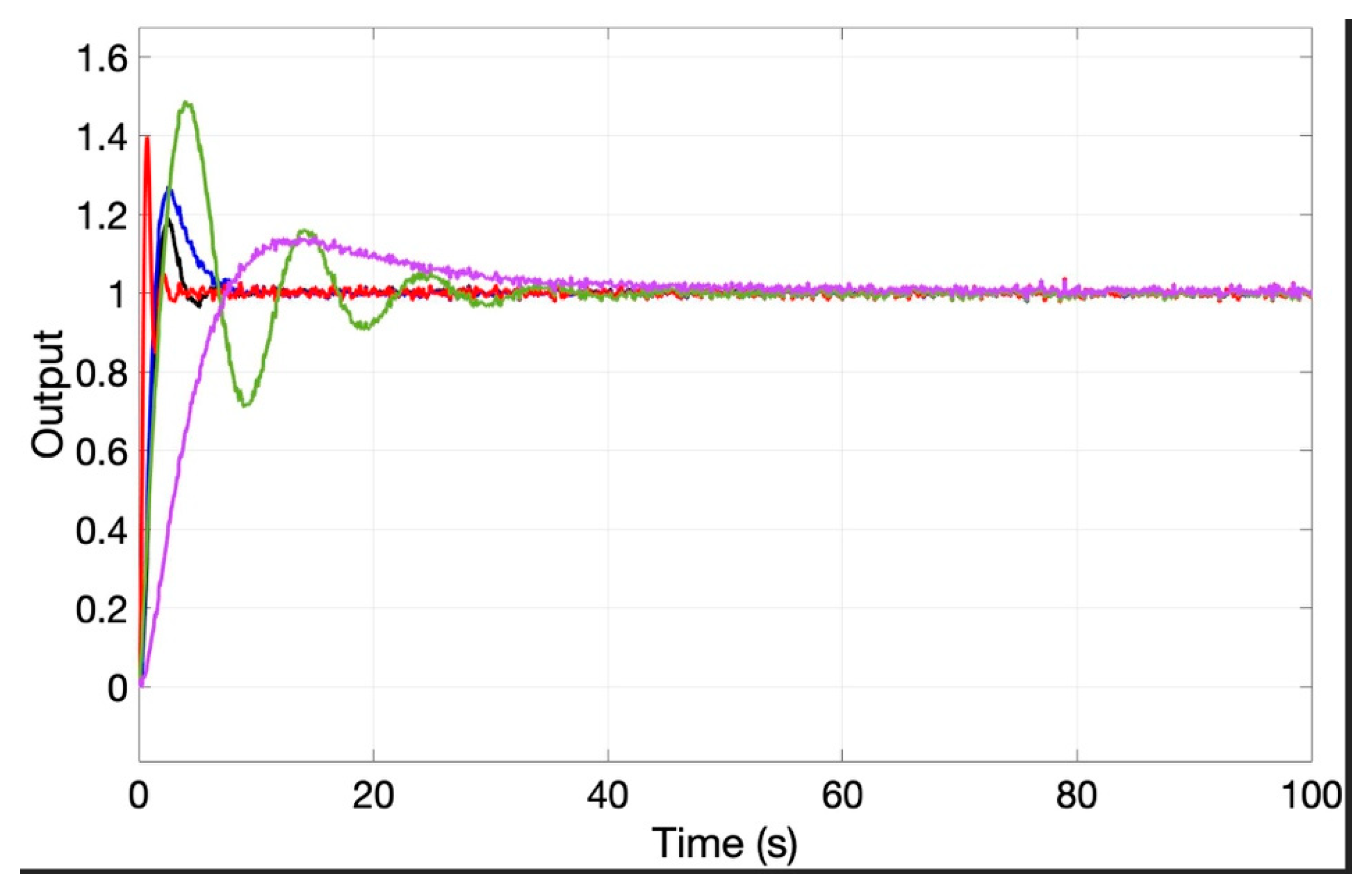
The closed-loop simulation results for reference tracking are indicated in Figure 22. The quantitative performance results are included in

Table 2. FO-PID controllers’ performance for reference tracking.

Controller	Overshoot	Settling Time	Mean-Squared Error
FO-PI in series with FO-PD [43]	27%	6.5	111.04
FO-PID ZN-FOC [44]	40%	2.3	52.64
FO-PID ZN-FOC [45]	48.5%	30.7	211.9
FO-PI [6]	15%	42	332.2
FO-PI using the RDR	18%	3.9	109.75

. The control signal required by the controller in (24) is considerably large. For the simulations, a saturated control signal in the range [−50, 50] has been considered. The closed-loop results show that the proposed tuning method offers good results in terms of reference tracking with a small overshoot comparable to that achieved by the FO-PI [6] and a fast settling time comparable to FO-PID in [44]. Note that the latter is a more complex fractional-order controller that includes the derivative action.

Figure 23 presents the comparative disturbance attenuation results considering a swept sine of amplitude 0.2 and frequency ranging [$0.5{\omega }_d, 2{\omega }_d$]. The mean-squared errors in this case are indicated in

Table 3. Mean-squared errors for swept sine disturbance.

FO-PI in Series with FO-PD [43]	FO-PID ZN-FOC [44]	FO-PID ZN-FOC [45]	FO-PI [6]	FO-PI Using the RDR
280.75	230.35	1.4 × 103	1.6 × 104	58.85

. The results show that the FO-PI designed according to the proposed method ensures the best performance, with approximately 75% improvement in attenuating stochastically varying disturbances compared to the next best fractional-order controller, the FO-PID designed according to [44].

4.7. An Unstable Time Delay Process

An unstable process is considered next [46]:

$$H_p\left(s\right)=\frac{1}{\left(s-1\right)}{e}^{-0.2s}$$

(25)

Optimal tuning rules for FO-PID controllers have been developed in [46], where the transfer function in (5) is altered to include a derivative filter, as well. The method is based on the minimization of the integrated absolute error. Two dedicated FO-PIDs are computed in [46] to control the process in (25):

$$H_{\mathrm{FOPID}1}\left(s\right)=6.94\left(1+1.29s^{-1}+0.0576s^{\mu }\right)\frac{1}{0.0089s+1}$$

(26)

$$H_{\mathrm{FOPID}2}\left(s\right)=6.19\frac{0.84s+1}{0.84s}\frac{0.07s^{1.193}+1}{0.01s+1}$$

(27)

An optimal PID controller is also designed in [46] for the process in (25), and the transfer function is given as:

$$H_{\mathrm{PID}}\left(s\right)=6.19\frac{0.84s+1}{0.84s}\frac{0.07s^{1.193}+1}{0.01s+1}$$

(28)

An FO-PI has been designed using the proposed method to ensure similar setpoint tracking results as the FO-PIDs in (26) by imposing a PM = 23° and ${\omega }_c=3.3$ rad/s. The integral gain k_i is then computed according to (14) for $\lambda \in \left(0÷1\right)$. The proportional gain k_p is then determined based on (15) for each pair ($\lambda$, k_i). The RDR is then evaluated at a frequency of interest ${\omega }_d=0.85$ rad/s, and the result is given in Figure 24. The maximum RDR value is obtained for $\lambda =0.9$; thus, k_i = 0.67 and k_p = 3.25. The performance of the proposed FO-PI controller is compared to that obtained using the two FO-PIDs from [46]. To implement the fractional-order controllers, the NRTF approach is used [41], with N = 5, $\alpha =0.9$ and $T_s=0.2 \mathrm{s}$.

The closed-loop simulation results for reference tracking are indicated in Figure 25. The two FO-PID controllers exhibit extra tuning parameters compared to the FO-PI controller, which allowed for a finer tuning with possibly better closed-loop performance. The same is valid for the PID controller in (28), which has one supplementary tuning parameter compared to the FO-PI. At the same time, notice that all controllers in (26)–(28) exhibit derivative action that leads to a reduce settling time and improves the stability of the overall control system. As indicated in [46], the required control efforts are very large, with amplitudes exceeding 50. For a fair comparison with the FO-PI controller, all inputs were bounded in the [−4, +4] range. Additive noise is considered on the output of the process to be controlled. As seen in Figure 25, the overshoot obtained with the FO-PI controller is similar to that obtained with the PID in (28). Due to noise, the performance of the FO-PIDs has obviously degraded, with an increased overshoot. The proposed FO-PI controller achieves similar performance in terms of overshoot, compared to the other three controllers. However, due to the derivative term, the controllers in (26)–(28) achieve better settling times in the range of 2.1–2.3 s, compared to the FO-PI with a 4 s settling time. All three controllers in (26)–(28) have been designed specifically for the process in (25) by optimizing the closed-loop performance. Nevertheless, the reference tracking results show that the proposed method can be used to stabilize an unstable time delay process, with decent closed-loop performance.

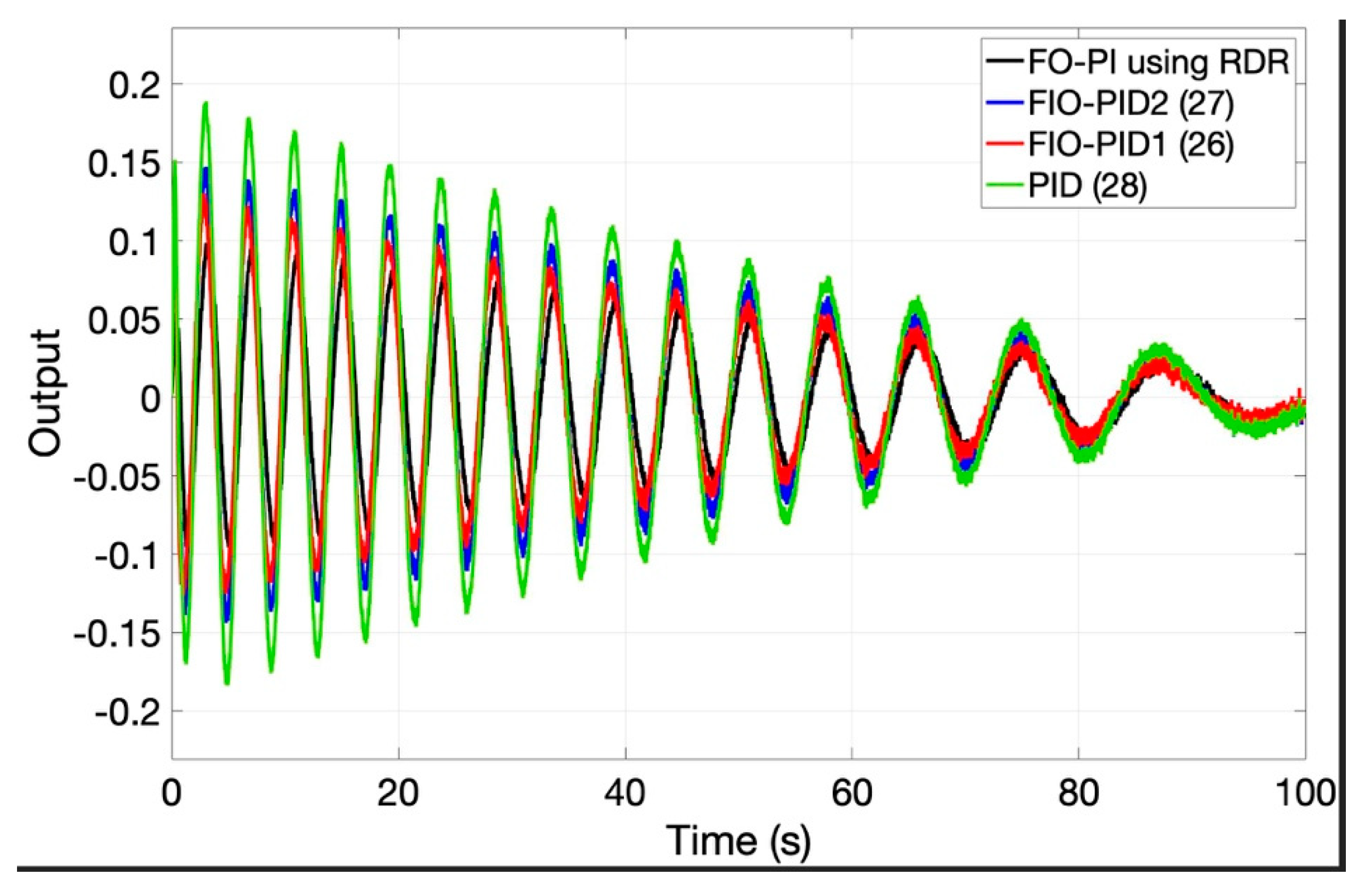
Figure 26 shows the disturbance rejection results obtained using the proposed FO-PI and the two FO-PIDs in (26) and (27), as well as the PID in (28). A swept sine of amplitude 0.2 and frequency ranging [$0.25{\omega }_d, 2{\omega }_d$] is considered. The mean-squared error in this case is 90.23 for the proposed method, 181 for the FO-PID in (27), 131 for the FO-PID in (26) and 293 for the PID in (28). This accounts for 31% improvement in attenuating stochastically varying disturbances compared to the FO-PID in (26), 51% improvement compared to the FO-PID in (27) and 69% improvement compared to the PID in (28). The results clearly show that the ability of the controllers to reduce stochastically varying disturbances is greatly improved using the RDR as a design specification and the proposed method.

5. Conclusions

The presence of disturbances in practical control engineering applications is unavoidable. Unfortunately, the disturbances also have a negative impact upon the control system. As such, apart from reference tracking, control systems have to be properly designed in order to ensure a decent robust disturbance rejection. Research on fractional-order controllers lead to the conclusion that these offer an improvement of the closed-loop results, as well as increased robustness, compared to the classical integer-order controllers.

Stepwise disturbances are not sufficient to evaluate a controller’s performance. The purpose of this study was to introduce a novel tuning method for fractional-order controllers, with the aim of improving the disturbance attenuation of periodic disturbances. The tuning method uses the reference–to–disturbance ratio as a quantitative measure of the control system’s ability to reject such external signals. The method requires knowledge about or an estimation of the main frequency of the disturbance signal.

Six numerical examples are provided. The first is intended to justify the need for using the RDR measure in the design. It is shown that a control system with a larger RDR value is able to diminish the effect of the disturbance, compared to a control system with a smaller RDR value. The second numerical example shows that a fractional-order controller can, in some cases, improve the disturbance attenuation compared to a classical integer-order controller. The third example shows the robustness of the proposed tuning method. The simulation results provide for a validation of the proposed tuning method. The fourth example shows that the proposed method is suitable also for more complex processes as it provides good reference tracking and better disturbance rejection. The results are compared with those of an FO-PI controller tuned according to an extended Ziegler–Nichols method for fractional-order controllers. The fifth and sixth examples consider integrating and unstable time delay processes. The results are compared to various fractional-order controllers, as well as an optimally tuned PID. Although in some cases, the proposed tuning method does not ensure the best reference tracking results compared to existing methods, the simulations results show that considering the RDR as a design specification improves the periodic disturbance attenuation properties of the fractional-order controllers.

Further research includes the extension of this method to FO-PID controllers, as well as experimental results. Additional improvements to the algorithm can also be considered, such as tackling better the issue of robustness by replacing the PM specification with the maximum sensitivity.

References

- Sira-Ramírez, H.; Luviano-Juárez, A.; Ramírez-Neria, M.; Zurita-Bustamante, E.W. Active Disturbance Rejection Control of Dynamic Systems; Butterworth-Heinemann: Oxford, UK, 2017; pp. 1–11. [Google Scholar]
- Alagoz, B.B.; Deniz, F.N.; Keles, C.; Tan, N. Disturbance rejection performance analyses of closed loop control systems by reference to disturbance ratio. ISA Trans. 2015, 55, 63–71. [Google Scholar] [CrossRef] [PubMed]
- Podlubny, I. Fractional-order systems and PIλDμ-controllers. IEEE Trans. Autom. Control 1999, 44, 208–214. [Google Scholar] [CrossRef]
- Chen, P.; Luo, Y.; Peng, Y.; Chen, Y.Q. Optimal robust fractional order PIλD controller synthesis for first order plus time delay systems. ISA Trans. 2021, 114, 136–149. [Google Scholar] [CrossRef] [PubMed]
- Dabiri, A.; Moghaddam, B.P.; Machado, J.A.T. Optimal variable-order fractional PID controllers for dynamical systems. J. Comput. Appl. Math. 2018, 339, 40–48. [Google Scholar] [CrossRef]
- Monje, C.A.; Chen, Y.; Vinagre, B.M.; Xue, D.; Feliu-Batlle, V. Fractional-Order Systems and Controls: Fundamentals and Applications; Springer Science & Business Media: Berlin/Heidelberg, Germany, 2010. [Google Scholar]
- Tepljakov, A. Fractional-Order Modeling and Control of Dynamic Systems; Springer: Berlin/Heidelberg, Germany, 2017. [Google Scholar]
- Lanchier, N. Stochastic Modeling; Springer: Berlin/Heidelberg, Germany, 2017. [Google Scholar]
- Butler, H.; Honderd, G.; van Amerongen, J. Model reference adaptive control of a direct-drive DC motor. IEEE Control Syst. Mag. 1989, 9, 80–84. [Google Scholar] [CrossRef]
- Castillo, A.; Sanz, R.; Garcia, P.; Albertos, P. Robust Design of the Uncertainty and Disturbance Estimator. IFAC-PapersOnLine 2017, 50, 8262–8267. [Google Scholar] [CrossRef]
- Lu, Q.; Ren, B.; Parameswaran, S. Uncertainty and Disturbance Estimator-Based Global Trajectory Tracking Control for a Quadrotor. IEEE/ASME Trans. Mechatron. 2020, 25, 1519–1530. [Google Scholar] [CrossRef]
- Furtat, I.B.; Chugina, J.V. Robust adaptive control with disturbances compensation. IFAC-PapersOnLine 2016, 49, 117–122. [Google Scholar] [CrossRef]
- Sun, L.; Sun, G. Robust Adaptive Saturated Fault-tolerant Control of Autonomous Rendezvous with Mismatched Disturbances. Int. J. Control Autom. Syst. 2019, 17, 2703–2713. [Google Scholar] [CrossRef]
- Yamamoto, T.; Takao, K.; Yamada, T. Design of a data-driven PID controller. IEEE Trans. Control Syst. Technol. 2008, 17, 29–39. [Google Scholar] [CrossRef]
- Barbosa, R.S.; Machado, J.T.; Ferreira, I.M. Tuning of PID controllers based on Bode’s ideal transfer function. Nonlinear Dyn. 2004, 38, 305–321. [Google Scholar] [CrossRef]
- Dazi, L.; Lang, L.; Qibing, J.; Hirasawa, K. Maximum sensitivity based fractional IMC–PID controller design for non-integer order system with time delay. J. Process Control 2015, 31, 17–29. [Google Scholar]
- Anantachaisilp, P.; Lin, Z. Fractional Order PID Control of Rotor Suspension by Active Magnetic Bearings. Actuators 2017, 6, 4. [Google Scholar] [CrossRef] [Green Version]
- Ranganayakulu, R.; Babu, G.U.B.; Rao, A.S.; Patle, D.S. A comparative study of fractional order PIλ/PIλDµ tuning rules for stable first order plus time delay processes. Resour. Effic. Technol. 2016, 2, S136–S152. [Google Scholar] [CrossRef]
- Magin, R.; Ortigueira, M.D.; Podlubny, I.; Trujillo, J. On the fractional signals and systems. Signal Process. 2011, 91, 350–371. [Google Scholar] [CrossRef]
- Shamsuzzoha, M.; Lee, M. IMC-PID Controller Design for Improved Disturbance Rejection of Time-Delayed Processes. Ind. Eng. Chem. Res. 2007, 46, 2077–2091. [Google Scholar] [CrossRef]
- Visioli, A. A new design for a PID plus feedforward controller. J. Process Control 2004, 14, 457–463. [Google Scholar] [CrossRef]
- Su, W.A. Model Reference-Based Adaptive PID Controller for Robot Motion Control of Not Explicitly Known Systems. Int. J. Intell. Control Syst. 2007, 12, 237–244. [Google Scholar]
- Trajkov, N.T.; Köppe, H.; Gabbert, U. Direct model reference adaptive control (MRAC) design and simulation for the vibration suppression of piezoelectric smart structures. Commun. Nonlinear Sci. 2008, 13, 1896–1909. [Google Scholar] [CrossRef]
- Tian, Y.; Zhao, Y.; Shi, Y.; Cao, X.; Yu, D.-L. The Indirect Shared Steering Control Under Double Loop Structure of Driver and Automation. IEEE/CAA J. Autom. Sin. 2020, 7, 1403–1416. [Google Scholar]
- Yang, Y.; Tan, J.; Yue, D. Prescribed Performance Control of One-DOF Link Manipulator with Uncertainties and Input Saturation Constraint. IEEE/CAA J. Autom. Sin. 2019, 6, 148–157. [Google Scholar] [CrossRef]
- Zheng, Q.; Gao, Z. On practical applications of active disturbance rejection control. In Proceedings of the 29th Chinese Control Conference, Beijing, China, 29–31 July 2010; pp. 6095–6100. [Google Scholar]
- Tan, W.; Fu, C. Analysis of active disturbance rejection control for processes with time delay. In Proceedings of the 2015 American Control Conference (ACC), Chicago, IL, USA, 1–3 July 2015; pp. 3962–3967. [Google Scholar] [CrossRef]
- Guo, B.-Z.; Zhao, Z.-L. On convergence of the nonlinear active disturbance rejection control for MIMO systems. SIAM J. Control Optim. 2013, 51, 1727–1757. [Google Scholar] [CrossRef]
- Guo, B.-Z.; Zhao, Z.-L. On the convergence of an extended state observer for nonlinear systems with uncertainty. Syst. Control Lett. 2011, 60, 420–430. [Google Scholar] [CrossRef]
- Zheng, Q.; Gao, L.; Gao, Z. On stability analysis of active disturbance rejection control for nonlinear time-varying plants with unknown dynamics. In Proceedings of the IEEE Conference on Decision and Control, New Orleans, LA, USA, 12–14 December 2017; pp. 12–14. [Google Scholar]
- Dazi, L.; Pan, D.; Gao, Z. Fractional active disturbance rejection control. ISA Trans. 2016, 62, 109–119. [Google Scholar]
- Fang, H.; Yuan, X.; Liu, P. Active–disturbance–rejection–control and fractional–order–proportional–integral–derivative hybrid control for hydroturbine speed governor system. Meas. Control 2018, 51, 192–201. [Google Scholar] [CrossRef] [Green Version]
- Chen, P.; Luo, Y.; Zheng, W.; Gao, Z.; Chen, Y.Q. Fractional order active disturbance rejection control with the idea of cascaded fractional order integrator equivalence. ISA Trans. 2021, 114, 359–369. [Google Scholar] [CrossRef]
- Zheng, W.; Luo, Y.; Chen, Y.; Wang, X. A Simplified Fractional Order PID Controller’s Optimal Tuning: A Case Study on a PMSM Speed Servo. Entropy 2021, 23, 130. [Google Scholar] [CrossRef]
- Tepljakov, A.; Alagoz, B.B.; Gonzalez, E.; Petlenkov, E.; Yeroglu, C. Model Reference Adaptive Control Scheme for Retuning Method-Based Fractional-Order PID Control with Disturbance Rejection Applied to Closed-Loop Control of a Magnetic Levitation System. J. Circuits Syst. Comput. 2018, 27, 1850176. [Google Scholar] [CrossRef]
- Costa-Castelló, R.; Olm, J.M.; Ramos, G.A. Design and analysis strategies for digital repetitive control systems with time-varying reference/disturbance period. Int. J. Control 2011, 84, 1209–1222. [Google Scholar] [CrossRef]
- Ozbey, N.; Yeroglu, C.; Alagoz, B.B.; Herencsar, N.; Kartci, A.; Sotner, R. 2DOF multi-objective optimal tuning of disturbance reject fractional order PIDA controllers according to improved consensus oriented random search method. J. Adv. Res. 2020, 25, 159–170. [Google Scholar] [CrossRef]
- Chu, M.; Chu, J. Graphical Robust PID Tuning Based on Uncertain Systems for Disturbance Rejection Satisfying Multiple Objectives. Int. J. Control Autom. Syst. 2018, 16, 2033–2042. [Google Scholar] [CrossRef]
- Deniz, F.N.; Keles, C.; Alagoz, B.B.; Tan, N. Design of fractional-order PI controllers for disturbance rejection using RDR measure. In Proceedings of the ICFDA’14 International Conference on Fractional Differentiation and Its Applications 2014, Catania, Italy, 23–25 June 2014; pp. 1–6. [Google Scholar] [CrossRef]
- Muresan, C.I.; Birs, I.R.; Ionescu, C.M.; de Keyser, R. Tuning of fractional order proportional integral/proportional derivative controllers based on existence conditions. Proc. IMechE Part I J. Syst. Control. Eng. 2019, 223, 384–391. [Google Scholar] [CrossRef]
- De Keyser, R.; Muresan, C.I.; Ionescu, C.M. An efficient algorithm for low-order discrete-time implementation of fractional order transfer functions. ISA Trans. 2018, 74, 229–238. [Google Scholar] [CrossRef] [PubMed]
- Gude, J.J.; Kahoraho, E. Modified Ziegler-Nichols method for fractional PI controllers. In Proceedings of the 2010 IEEE 15th Conference on Emerging Technologies & Factory Automation (ETFA 2010), Bilbao, Spain, 13–16 September 2010; pp. 1–5. [Google Scholar]
- Monje, C.A.; Vinagre, B.M.; Feliu, V.; Chen, Y.Q. On Auto-Tuning Of Fractional Order PIλDμ Controllers. In Proceedings of the 2nd IFAC Workshop on Fractional Differentiation and Its Application (FDA 06), Porto, Portugal, 19–21 July 2006. [Google Scholar]
- Muresan, C.I.; De Keyser, R. Revisiting Ziegler-Nichols. A fractional order approach. ISA Trans. 2022. [Google Scholar] [CrossRef]
- Valério, D.; Sá da Costa, J. Tuning rules for fractional PID controllers. IFAC Proc. 2006, 39, 28–33. [Google Scholar] [CrossRef]
- Padula, F.; Visioli, A. Optimal tuning rules for proportional-integral-derivative and fractional-order proportional-integral-derivative controllers for integral and unstable processes. IET Control Theory Appl. 2012, 6, 776–786. [Google Scholar] [CrossRef]
Figure 1.
Closed-loop system diagram.
Figure 2.
Tuning algorithm of FO-PI controllers for improved disturbance attenuation.
Figure 3.
RDR values corresponding to two different FO-PI controllers.
Figure 4.
Disturbance rejection results for two different FO-PI controllers for a 0.8 rad/s disturbance frequency.
Figure 5.
Disturbance rejection results for two different FO-PI controllers for a 0.2 rad/s disturbance frequency.
Figure 6.
RDR vs. for example 1.
Figure 7.
RDR vs. disturbance signal frequency spectra for a simple first-order process.
Figure 8.
Comparative reference tracking results for a simple first-order system.
Figure 9.
Comparative disturbance rejection results for a simple first-order system.
Figure 10.
RDR vs. for a first-order plus dead-time process.
Figure 11.
Reference tracking results for a first-order plus dead-time process.
Figure 12.
Disturbance rejection results for a first-order plus dead-time process considering a sinusoidal disturbance signal of frequency .
Figure 13.
Robustness of the designed fractional-order controller to sinusoidal disturbance frequency variations.
Figure 14.
RDR vs. disturbance frequency signal spectra for an FOPDT process.
Figure 15.
Robustness of a suboptimal fractional-order controller to sinusoidal disturbance frequency variations.
Figure 16.
RDR vs. for a higher-order process.
Figure 17.
Reference tracking results for higher-order process (red line—FO-PI designed by Gude 2010).
Figure 18.
Disturbance rejection results for a higher-order process considering a sinusoidal disturbance signal of frequency (red line—FO-PI designed by Gude 2010).
Figure 19.
Load disturbance rejection results for a higher-order process (red line—FO-PI designed by Gude 2010).
Figure 20.
Disturbance rejection results for a higher-order process considering a swept sinusoidal disturbance signal with frequencies in [] (red line—FO-PI designed by Gude 2010).
Figure 21.
RDR vs. for an integrating time delay process.
Figure 22.
Reference tracking results for integrative time delay process (black line—FO-PI deisgned using the RDR, blue line—FO-PID designed by Monje 2006, red line—FO-PID designed by Muresan 2022, green line—FO-PID designed by Valerio 2006, magenta line—FO-PI designed by Monje 2010).
Figure 23.
Disturbance rejection results for an integrative time delay process considering a swept sinusoidal disturbance signal with frequencies in [] (black line–FO-PI deisgned using the RDR, blue line–FO-PID designed by Monje 2006, red line–FO-PID designed by Muresan 2022, green line–FO-PID designed by Valerio 2006, magenta line–FO-PI designed by Monje 2010).
Figure 24.
RDR vs. for an unstable time delay system.
Figure 25.
Reference tracking results for an unstable time delay process.
Figure 26.
Disturbance rejection results for an unstable time delay process considering a swept sinusoidal disturbance signal with frequencies in [].